Heralded quantum repeater for a quantum communication network based on quantum dots embedded in optical microcavities

Abstract

We propose a heralded quantum repeater protocol based on the general interface between the circularly polarized photon and the quantum dot embedded in a double-sided optical microcavity. Our effective time-bin encoding on photons results in the deterministic faithful entanglement distribution with one optical fiber for the transmission of each photon in our protocol, not two or more. Our efficient parity-check detector implemented with only one input-output process of a single photon as a result of cavity quantum electrodynamics makes the entanglement channel extension and entanglement purification in quantum repeater far more efficient than others, and it has the potential application in fault-tolerant quantum computation as well. Meanwhile, the deviation from a collective-noise channel leads to some phase-flip errors on the nonlocal electron spins shared by the parties and these errors can be depressed by our simplified entanglement purification process. Finally, we discuss the performance of our proposal, concluding that it is feasible with current technology.

I introduction

The reliable transmission of quantum states over noisy channels is important in quantum communication, such as quantum teleportation teleportation , dense coding Densecoding ; Densecoding1 , quantum key distribution QKD ; QKD1 ; collectivenoiselixhQKD , quantum secret sharing QSS ; QSS1 ; QSS2 , and quantum secure direct communication QSDC1 ; QSDC2 ; QSDC3 . However, serious problems occur when long-distance quantum communication is considered noise . Due to the exponential scaling photon loss in the transmission channel, the success probability of the direct transmission for photons over a $1000$-km optical fiber is of order $10^{-20}$. Even though the photon can arrive at the receiver, the fidelity of its polarization state also decreases largely, due to the random birefringence arising from thermal fluctuations, vibrations, and imperfections of the fiber itself. To establish a long-distance entanglement channel, a quantum repeater protocol was originally proposed by Briegel et al. Qrepeater0 in 1998 to reduce the photon loss rate and suppress the decoherence of entangled photon pairs. Some interesting proposals for quantum repeaters have been proposed in various physical systems, such as nitrogen vacancy (NV) centers in diamond high-frep1 ; high-frep2 ; qqentangle1 , atomic ensembles repeaternature ; repeaterPRL ; revqr , and single trapped ions ionqr .

Considering the long electron-spin coherence time [$\mu$s is achieved in both a quantum dot (QD) ensemble and a single QD], fast manipulation, and easy scalability, QD is one of the good candidates for local storage and processing of quantum information. Single semiconductor QD coupling to a microcavity has attracted much attention Qdcoupling3 ; weihairuiOE2 ; wanghongfuPRA ; RenbaocangSR ; renHEPPPRA ; Qdcoupling4 ; Qdcoupling0 ; Qdqr1 ; Qdqr2 ; Qdqr3 ; qqentangle2 . The giant circular birefringence originated from the spin selective dipole coupling for such spin-cavity systems is utilized in photon-photon or spin-photon entanglement generation Qdcoupling3 , hyper-parallel quantum computing RenbaocangSR , universal quantum gates Qdcoupling0 ; weihairuiOE2 ; wanghongfuPRA , hyperentanglement purification and concentration renHEPPPRA , and complete Bell-state analyzers Qdcoupling4 . In 2006, Waks and Vuckovic put forward a quantum repeater scheme with the QD-cavity system Qdqr1 . The entanglement creation between neighboring QDs and the subsequently entanglement swapping were assisted by the QD-induced transparency of the coherent field, which is faithful when the photon number resolved detectors were available. In 2007, Simon et al. Qdqr2 proposed a scheme for entangling two remote spins based on two-photon coincidence detection and they constituted a controlled-phase gate between two local spins with the dipole-dipole interaction between trions in neighboring QDs. This gate makes the quantum entanglement swapping possible and it leads to the realization of a quantum repeater. In 2012, the error-free entanglement distribution was performed with the momentum-entangled photons and the QDs embedded in microcavities when the momentum entanglement is stable Qdqr3 . Recently, Jones et al. qqentangle2 proposed an efficient scheme to entangle remotely separated QDs with a midpoint-entanglement source and one nondeterministic Bell-state measurement located at each end of the two channels, which was used to complete the entanglement swapping between the QD-photon entanglement Qdphoton1 ; Qdphoton2 ; Qdphoton3 and the photon-photon entanglement, resulting in the entanglement between QDs.

Since the seminal work about Bell inequality for position and time by Franson time-bin1 , the time-bin degree of freedom (DOF) of photons has attracted much attention time-bin2 ; time-bin3 ; lixhapl ; time-bin4 ; time-bin5 ; time-bin6 ; time-bin7 . The two-photon time-bin entanglement source for quantum communication was demonstrated by Brendel et al. time-bin2 in 1999. With the encoded time-bin qubits, Kalamidas time-bin3 proposed a single-photon quantum error-rejection transmission protocol in 2005, in which a probabilistic transmission is completed with two Pockels cells (PCs) and the deterministic error-free transmission is performed with four PCs. In 2007, Li et al. lixhapl proposed a faithful qubit transmission scheme against collective noise without ancillary qubits, resorting to the time-bin DOF of a single photon itself. Recently, the distribution of time-bin entangled qubits time-bin4 over an optical fiber at the scale of 300 km time-bin5 was demonstrated and the two-photon interference fringes exhibited a visibility of 84%. A time-bin qubit can also be used to perform quantum computing time-bin6 and only a single optical path rather than multiple paths is used to complete single-qubit operations and herald controlled-phase gates. An ultrafast measurement technique for time-bin qubits time-bin7 was implemented, which makes time-bin qubits more useful time-bin8 .

In this paper, we show that a heralded quantum repeater based on the QD-microcavity systems can be constructed with the help of the effective time-bin encoder and the general interface between the circularly polarized photon and the QD embedded in a double-sided optical microcavity. By using the giant circular birefringence effect for the singly charged QD inside a microcavity and the two-photon coincident measurement, the time-bin entanglement can be converted deterministically into that of the remotely located QD-electron-spin system in a heralded way. The entanglement distribution can in principle be performed with a unity efficiency when none of the photons are lost during the transmission process. It is more efficient than others Qdqr2 ; qqentangle2 if the multimode process is involved QRmulti-spatial ; qqentangle2 . Our efficient parity-check detector (PCD) implemented with only one input-output process of a single photon as a result of cavity quantum electrodynamics makes the entanglement channel extension and entanglement purification in our quantum repeater far more efficient than others. The deviation from collective noise channel leads to some phase-flip errors that can be suppressed by our simpler entanglement purification process. These features make our heralded quantum repeater protocol more useful in the quantum communication network in the future.

This paper is organized as follows: We give a general interface between a circularly polarized light and a QD-cavity system in Sec. II.1. Subsequently, we present the faithful entanglement distribution for two neighboring nodes in Sec. II.2, and then, we give an efficient way to complete the entanglement extension with a PCD in Sec. II.3. In Sec. III, we propose an efficient entanglement purification protocol to depress the influence of asymmetric noise from optical-fiber channels on different time bins. In Sec. IV, we discuss the influence from the practical imperfect circular birefringence on the created entanglement. A discussion and a summary are given in Sec. V. In addition, $N$-user entanglement distribution for a multiuser quantum repeater network is discussed in Appendix A.

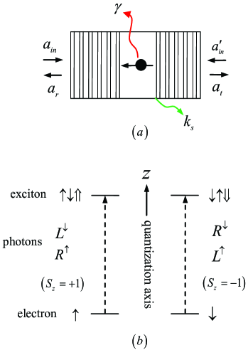
Figure 1: The spin-dependent transitions for a negatively charged exciton $X^{-}$. (a) A singly charged QD inside a double-sided optical microcavity. (b) The spin selection rules for optical transition of a negatively charged exciton. The symbols $\uparrow$ and $\downarrow$ represent the excess electron-spin projections $|+\frac{1}{2}\rangle$ and $|-\frac{1}{2}\rangle$ along the quantization axis ($z$-direction), respectively. The symbols $\Uparrow$ and $\Downarrow$ represent the spin projections of the hole $|+\frac{3}{2}\rangle$ and $|-\frac{3}{2}\rangle$, respectively. $R^{\uparrow}$ ($L^{\downarrow}$) denotes a right-circularly (a left-circularly) polarized photon propagating along (against) the quantization axis.

II faithful entanglement distribution and extension for heralded quantum repeater

II.1 The interface between a circularly polarized light and a QD-cavity system

Let us consider a singly charged QD (e.g., for a self-assembled InAs/GaAs quantum dot) embedded inside a resonant double-sided micropillar cavity Qdcoupling3 . Both the top and bottom mirrors of the cavity are partially reflective, shown in Fig. 1(a). The optical properties of a singly charged QD embedded inside a micropillar cavity are dominated by the optical transitions of the negatively charged trion ($X^{-}$) that consists of two electrons bounded to one hole Qdchar , shown in Fig.1(b). When the quantization axis for angular momentum is the $z$ axis for the QD geometry, the single electron states have the spin $J_{z}=\pm\frac{1}{2}$ (labeled as $|\uparrow\rangle$ and $|\downarrow\rangle$), and the hole $J_{z}=\pm\frac{3}{2}$ (labeled as $|\Uparrow\rangle$ and $|\Downarrow\rangle$). Photon polarization ($L$ and $R$ represent the left and the right circularly polarized states of photons, respectively) is defined with respect to the direction of the propagation, and this causes the polarization to change upon reflection. In a trion state, due to the Pauli’s exclusion principle, the two electrons form a singlet state with the total spin zero, which decouples the interaction between the electron spin and the hole spin Qdchar ; Qdchartri . In other words, the circularly polarized photon directed into the spin-cavity system can either be coupled with the electron spin and feels a hot cavity when the dipole selection rule is fulfilled, or be decoupled and feels a cold cavity in the other case. The significant difference in the reflection and the transmission coefficients manifested between these two cases is spin dependent, and it can be exploited to perform the quantum information processing Qdcoupling3 ; weihairuiOE2 ; wanghongfuPRA ; RenbaocangSR ; renHEPPPRA ; Qdcoupling4 ; Qdcoupling0 ; Qdqr1 ; Qdqr2 .

The reflection and the transmission coefficients of this spin-cavity system can be obtained by solving the Heisenberg equations of motion for the cavity field operator $\hat{a}$ and the trion dipole operator $\hat{\sigma}_{-}$ along with the input-output relations Qdqr1 ; doubleEq ; singleEq .

$$\begin{split}\frac{d\hat{a}}{dt}\;=\;\;&-\left(i\omega_{c}+\kappa+\frac{\kappa_{s}}{2}\right)\hat{a}-ig\hat{\sigma}_{-}\\ &-\sqrt{\kappa_{s}}\,\hat{s}_{in}-\sqrt{\kappa}\,\hat{a}_{in}-\sqrt{\kappa}\,\hat{a}_{in}^{\prime},\\ \frac{d\hat{\sigma}_{-}}{dt}\;=\;\;&-\left(i\omega_{X^{-}}+\frac{\gamma}{2}\right)\hat{\sigma}_{-}+ig\hat{\sigma}_{z}\hat{a}+\sqrt{\gamma}\,\hat{\sigma}_{z}\hat{N},\;\;\;\;\;\;\\ \hat{a}_{r}\;=\;\;&\hat{a}_{in}+\sqrt{\kappa}\,\hat{a},\\ \hat{a}_{t}\;=\;\;&\hat{a}_{in}^{\prime}+\sqrt{\kappa}\,\hat{a}.\end{split}$$ (1)

Here $\hat{a}_{in}$ and $\hat{a}_{in}^{\prime}$ are the two input field operators. While $\hat{s}_{in}$ is an operator for an input field originating from potential leaky modes due to sideband leakage and absorption, and it associates with the corresponding output mode $\hat{s}_{out}$ by $\hat{s}_{out}=\hat{s}_{in}+\sqrt{\kappa_{s}}\hat{a}$ . $\hat{a}_{r}$ and $\hat{a}_{t}$ are the two output field operators, shown in Fig.1(a). $\hat{N}$ is the corresponding vacuum noise operator which helps to preserve the desired commutation relations for the QD-dipole operators. $\omega$, $\omega_{c}$, and $\omega_{X^{-}}$ are the frequencies of the input photon, cavity mode, and $X^{-}$ transition, respectively. $\kappa$ and $\kappa_{s}$ are the cavity-field decay rate and the side-leakage rate, respectively. $g$ is the coupling strength between $X^{-}$ and the cavity mode. $\gamma/2$ is the dipole decay rate. In the limit of weak incoming field, the charged QD is predominantly in the ground state in the whole process, that is, $<\hat{\sigma}_{z}>\approx-1$. The spin-cavity system behaves like a beam splitter whose reflection and transmission coefficients $R(\omega)$ and $T(\omega)$ along with the leakage and noise coefficients $S(\omega)$ and $N(\omega)$ are detailed, respectively, by:

$$\begin{split}R(\omega)\;\;=\;\;&\frac{i(\omega_{c}-\omega)+\frac{\kappa_{s}}{2}+\frac{g^{2}}{i(\omega_{X^{-}}-\omega)+\frac{\gamma}{2}}}{i(\omega_{c}-\omega)+\kappa+\frac{\kappa_{s}}{2}+\frac{g^{2}}{i(\omega_{X^{-}}-\omega)+\frac{\gamma}{2}}},\\ T(\omega)\;\;=\;\;&\frac{-\kappa}{i(\omega_{c}-\omega)+\kappa+\frac{\kappa_{s}}{2}+\frac{g^{2}}{i(\omega_{X^{-}}-\omega)+\frac{\gamma}{2}}},\;\;\;\;\;\;\end{split}$$ (2)

and

$$\begin{split}S(\omega)\;\;=\;\;&\frac{-\sqrt{\kappa_{s}\kappa}}{i(\omega_{c}-\omega)+\kappa+\frac{\kappa_{s}}{2}+\frac{g^{2}}{i(\omega_{X^{-}}-\omega)+\frac{\gamma}{2}}},\\ N(\omega)\;\;=\;\;&\frac{\frac{ig\sqrt{\gamma\kappa}}{i(\omega_{X^{-}}-\omega)+\frac{\gamma}{2}}}{i(\omega_{c}-\omega)+\kappa+\frac{\kappa_{s}}{2}+\frac{g^{2}}{i(\omega_{X^{-}}-\omega)+\frac{\gamma}{2}}}.\;\;\;\;\;\;\end{split}$$ (3)

Here, one has $P(\omega)=|R(\omega)|^{2}+|T(\omega)|^{2}+|S(\omega)|^{2}+|N(\omega)|^{2}=1$ meaning that when the noise or environment is considered, the energy of the whole system is conserved during the input-output process described above, and it can be reduced to the simplified input-output models in doubleEq or Qdqr1 by omitting the leaky modes $\hat{s}_{in}$ or vacuum noise operator $\hat{N}$ that helps to preserve the desired commutation relations for the QD-dipole operators, respectively.

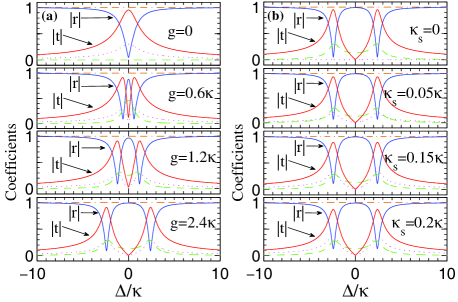
Figure 2: (Color online) The coefficients $|R(\omega)|$, $|T(\omega)|$, $|S(\omega)|$, $|N(\omega)|$, and $P(\omega)$ vs detuning $\Delta/\kappa$ (a) for different coupling strengths ($g=0$, $0.6\kappa$, $1.2\kappa$, and $2.4\kappa$) with $\kappa_{s}/\kappa=0.1$ and (b) for different leakage rates ($\kappa_{s}=0$, $0.05\kappa$, $0.15\kappa$, and $0.2\kappa$) with $g/\kappa=2.4$. $|R(\omega)|$ : solid blue line; $|T(\omega)|$: solid red line; $|S(\omega)|$: dot magenta line; $|N(\omega)|$: dashed green line; $P(\omega)$: dash-dash-dot brown line. Here $\Delta=\omega_{c}-\omega$. $\gamma/\kappa=0.1$ is taken by considering the typical QD micropillar parameters.

We are interested in the reflection and transmission of a single input photon that leads to the click of a single-photon detector, while the environment excitation inhibits the click. Therefore, we can project the output photon into the subspace spanned by the reflection and transmission modes. The state vector evolves on reflection and transmission as

$$\hat{a}_{in}^{\dagger}|S\rangle\;\rightarrow\;R\,\hat{a}_{r}^{\dagger}|S\rangle+T\,\hat{a}_{t}^{\dagger}|S\rangle.$$ (4)

For simplification, we take the case that the trion dipole is tuned into the cavity mode ($\omega_{c}=\omega_{X^{-}}$). When the input photon couples to the QD embedded in the microcavity, the coefficients $R$ and $T$ are reduced to $r(\Delta)$ and $t(\Delta)$, respectively. Here

$$\begin{split}r(\Delta)\;\;=\;\;&\frac{i\Delta+\frac{\kappa_{s}}{2}+\frac{g^{2}}{i\Delta+\frac{\gamma}{2}}}{i\Delta+\kappa+\frac{\kappa_{s}}{2}+\frac{g^{2}}{i\Delta+\frac{\gamma}{2}}},\\ t(\Delta)\;\;=\;\;&\frac{-\kappa}{i\Delta+\kappa+\frac{\kappa_{s}}{2}+\frac{g^{2}}{i\Delta+\frac{\gamma}{2}}},\end{split}$$ (5)

where $\Delta=\omega_{c}-\omega$. When the input probe field is uncoupled to the dipole transition (i.e., $g=0$), the specific reflection and transmission coefficients can be simplified as

$$\begin{split}r_{0}(\Delta)\;\;=\;\;&\frac{i\Delta+\frac{\kappa_{s}}{2}}{i\Delta+\kappa+\frac{\kappa_{s}}{2}},\\ t_{0}(\Delta)\;\;=\;\;&\frac{-\kappa}{i\Delta+\kappa+\frac{\kappa_{s}}{2}}.\end{split}$$ (6)

For the condition $\Delta=0$, ${2g^{2}}/{\kappa\gamma}\gg 1$, and ${\kappa_{s}}/{2\kappa}\ll 1$, both the reflection coefficient $|r(\omega)|$ and the transmission coefficient $|t_{0}(\omega)|$ can approach $1$. Meanwhile, the noise terms $|S(\Delta)|\simeq\sqrt{\kappa_{s}/\kappa}$ and $|N(\Delta)|\simeq{}$$\sqrt{\kappa\gamma}/g$ can be neglected. However, the total probabilities for all channels that the input photon is scattered into by the QD-cavity system $P(\Delta)\equiv 1$ for any condition, shown in Fig. 2. To be exact, when we concern only the transmission and reflection modes, and the circularly polarized photon directed into the spin-cavity system is in the state $S_{z}=+1$ (i.e., $|L^{\downarrow}\rangle$ or $|R^{\uparrow}\rangle$), the excess electron in the state $|\uparrow\rangle$ will interact with the input photon, provide a hot cavity situation, and eventually make the photon be reflected. Upon reflection, both the polarization and the propagation direction of the photon will be flipped. However, if the input photon is in the state $|R^{\downarrow}\rangle$ or $|L^{\uparrow}\rangle$ ($S_{z}=-1$), it will be transmitted through the cavity and acquires an extra $\pi$ phase, leaving the electron spin state unaffected. The whole process can be summarized into the following transformations Qdcoupling0 :

$$\begin{split}|R^{\uparrow},\uparrow\rangle\;\rightarrow\;&|L^{\downarrow},\uparrow\rangle,\;\;\;\;|R^{\downarrow},\uparrow\rangle\;\rightarrow\;-|R^{\downarrow},\uparrow\rangle,\\ |L^{\downarrow},\uparrow\rangle\;\rightarrow\;&|R^{\uparrow},\uparrow\rangle,\;\;\;\;|L^{\uparrow},\uparrow\rangle\;\rightarrow\;-|L^{\uparrow},\uparrow\rangle.\end{split}$$ (7)

When the excess electron is in the state $|\downarrow\rangle$, the evolution can be described as Qdcoupling0 :

$$\begin{split}|R^{\uparrow},\downarrow\rangle\;\rightarrow\;&-|R^{\uparrow},\downarrow\rangle,\;\;\;\;\;\;\;\;|R^{\downarrow},\downarrow\rangle\;\rightarrow\;|L^{\uparrow},\downarrow\rangle,\\ |L^{\downarrow},\downarrow\rangle\;\rightarrow\;&-|L^{\downarrow},\downarrow\rangle,\;\;\;\;\;\;\;\;\,|L^{\uparrow},\downarrow\rangle\;\rightarrow\;|R^{\downarrow},\downarrow\rangle.\end{split}$$ (8)

Combining the rules above, we can accomplish the entanglement transfer from the nonlocal photon systems into the nonlocal spin systems and construct an efficient PCD which is essential for the entanglement purification of the spin systems and the entanglement extension in our quantum repeater protocol.

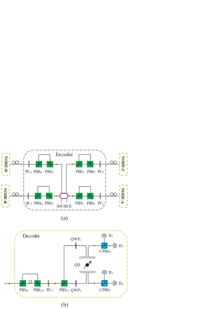
Figure 3: (Color online) Schematic architecture of the faithful entanglement distribution procedure in our quantum repeater protocol. (a) Deterministic and faithful entanglement distribution between the nodes A and B (A, B, $\cdots$, C and D) with the help of time-bin encoders. (b) The decoder for each quantum node. Here, the hexagon denotes the two-photon Bell source ($N$-photon GHZ source) and the orange rounded rectangles denoted with NODE-A and NODE-B represent the quantum nodes owned by the users Alice and Bob, respectively. PBS$\,{}_{i}$ ($i=1,2,\cdots$) is the polarizing beam splitter that transmits the $|H\rangle$ polarized photon and reflects the $|V\rangle$ polarized photon, respectively. QWP_j ($j=1,2$) represents a quarter-wave plate which is used to accomplish the transformations $|H\rangle\leftrightarrow|R\rangle$ and $|V\rangle\leftrightarrow|L\rangle$. CPBS_j represents the circularly polarizing beam splitter that transmits the $|R\rangle$ polarized photon and reflects the $|L\rangle$ polarized photon, respectively. PC$\,{}_{i}$ is a Pockels cell.

II.2 Faithful entanglement distribution for the quantum repeater network with time-bin encoders

To show how the spin-cavity system works for our deterministic entanglement distribution and our simplified entanglement purification protocol for quantum systems in a mixed entangled state explicitly, we first take the two-photon Bell state as an example, and then generalize it to the case with an $N$-photon Greenberger-Horne-Zeilinger (GHZ) state in Appendix A.

Suppose that there is a two-photon entangled source in the middle point of the two memory nodes belonging to the users, say Alice and Bob, shown in Fig. 3 (a). The photons $ab$ produced by the source are entangled in a Bell state in the polarization degree of freedom (DOF), i.e.,

$$|\Phi^{+}_{2}\rangle_{s}=\frac{1}{\sqrt{2}}\left(|H\rangle_{a}|H\rangle_{b}+|V\rangle_{a}|V\rangle_{b}\right),$$ (9)

where $|H\rangle$ and $|V\rangle$ represent the horizontal and the vertical polarization modes of photons, respectively. The subscripts $a$ and $b$ represent the photons transmitted to Alice and Bob, respectively. Before entering the noise channels, the photonic polarization entanglement is converted into the time-bin entanglement of the two photons $ab$ by passing the two photons through the encoders placed in their respective paths. Each encoder is made of two PBSs and a fast Pockels cell (PC). A PBS transmits the $|H\rangle$ polarized photon and reflects the $|V\rangle$ polarized one. A relative time delay $\Delta t$ of the nanoseconds scale can be obtained for the $|V\rangle$ component of the photon when the users appropriately preset the difference between the long optical path length $l$ of the $|V\rangle$ polarization photon and the short optical path length $s$ of the $|H\rangle$ polarization photon (i.e., the time interval of the unbalanced Mach-Zehnder interferometers). The parties turn on PC only when the $l$-path component appears and it is used to implement the bit-flip operation $|V\rangle\leftrightarrow|H\rangle$. After the encoders, the state of the system composed of photons $ab$ is changed into the time-bin entanglement with the polarization states all being $|H\rangle$,

$$|\Phi^{+}_{2}\rangle_{t_{0}}\!=\!\frac{1}{\sqrt{2}}|H\rangle_{a}|H\rangle_{b}(|s\rangle|s\rangle\!+\!|l\rangle|l\rangle)_{ab}.$$ (10)

Here $|s\rangle$ and $|l\rangle$ denote the early and late time bins with which the photon passes through the optical short ($s$) and long ($l$) paths, respectively.

Since all the photons in both $|s\rangle$ and $|l\rangle$ time bins launched into the noisy channels are in the $|H\rangle$ polarization, the influences of the collective noise on the photons in different time bins can be taken to be the same one time-bin3 ; lixhapl ; collectivenoise ; Yamamoto05 ; YamamotoExp2 . In other words, the noise of each optical-fiber channel is stable in the nanosecond scale that is just the time separation between the $|s\rangle$ and $|l\rangle$ time bins, and it can be expressed by a unitary transformation $U_{i}$,

$$U_{i}|H\rangle_{i}=\delta_{i}|H\rangle_{i}+\eta_{i}|V\rangle_{i}.$$ (11)

Here $|\delta_{i}|^{2}+|\eta_{i}|^{2}=1$. $i$ ($=a,b$) describes the noise on the photon $i$. The state of the photonic system $ab$ arriving at the two nodes, i.e., Alice and Bob, can be written as

$$|\Phi^{+}_{2}\rangle_{t_{1}}\!\! = \!\!\frac{1}{\sqrt{2}}(\delta_{a}|H\rangle_{a}\!+\!\eta_{a}|V\rangle_{a})(\delta_{b}|H\rangle_{b}\!+\!\eta_{b}|V\rangle_{b})$$ (12)

$$\!\!\!\otimes(|s\rangle_{a}|s\rangle_{b}\!+\!|l\rangle_{a}|l\rangle_{b}),$$

which is still a two-photon time-bin entanglement but the polarization state of the photonic system is ambiguous since the unitary transformation $U_{i}$ ($i=a,b$) on the photon $i$ is arbitrary and unknown for the parties in a quantum repeater.

The nodes NODE-A and NODE-B represent the two parties, Alice and Bob, respectively. They have the same device setting for their decoders, shown in Fig. 3 (b). After the photons pass through the unbalanced Mach-Zehnder interferometer composed of PBS₉ and PBS₁₀, a relative delay of $\Delta{}t$ on the $|H\rangle$ component is completed and the state of the photonic system evolves into

$$|\Phi^{+}_{2}\rangle_{t_{2}}\!\! = \!\!\frac{1}{\sqrt{2}}[\delta_{a}\delta_{b}|H\rangle_{a}|H\rangle_{b}(|sl\rangle_{a}|sl\rangle_{b}\!+\!|ll\rangle_{a}|ll\rangle_{b})$$ (13)

$$\!\!+\delta_{a}\eta_{b}|H\rangle_{a}|V\rangle_{b}(|sl\rangle_{a}|ss\rangle_{b}\!+\!|ll\rangle_{a}|ls\rangle_{b})$$

$$\!\!+\eta_{a}\delta_{b}|V\rangle_{a}|H\rangle_{b}(|ss\rangle_{a}|sl\rangle_{b}\!+\!|ls\rangle_{a}|ll\rangle_{b})$$

$$\!\!+\eta_{a}\eta_{b}|V\rangle_{a}|V\rangle_{b}(|ss\rangle_{a}|ss\rangle_{b}\!+\!|ls\rangle_{a}|ls\rangle_{b})],\;\;\;\;$$

and it is a partially polarized entangled state. The time-bin information heralds the polarization state of the photonic system, which can be utilized to correct the polarization error in the decoder with proper bit-flip operations. Here $|ij\rangle=|i\rangle|j\rangle$ and the notations $|i=s,l\rangle$ ($|j=s,l\rangle$) denote the corresponding time bins created in the encoder (decoder). PC_i at each node is supposed to be active only when the components of $|ls\rangle$ or $|s\,l\rangle$ time bins appear and implements the bit flip $|H\rangle\leftrightarrow|V\rangle$ for the components $|ls\rangle$ and $|s\,l\rangle$. PBS₁₁ transmits the $|H\rangle$ components and reflects the $|V\rangle$ components, respectively. Another relative time delay $\Delta{}t$ is exerted on the $|V\rangle$ components by setting a longer optical path for the $|V\rangle$ components. The state $|\Phi^{+}_{2}\rangle_{t_{2}}$ evolves to

$$|\Phi^{+}_{2}\rangle_{t_{3}} \!\!=\!\! \frac{1}{\sqrt{2}}(|H^{\uparrow}\rangle_{a}|H^{\uparrow}\rangle_{b}\!+\!|V^{\downarrow}\rangle_{a}|V^{\downarrow}\rangle_{b})$$ (14)

$$\otimes[(\delta_{a}|s^{\prime}\rangle_{a}\!+\!\eta_{a}|l^{\prime}\rangle_{a})(\delta_{b}|s^{\prime}\rangle_{b}\!+\!\eta_{b}|l^{\prime}\rangle_{b})].$$

Here the superscripts ${\downarrow}$ and ${\uparrow}$ represent the different outputs of PBS₁₁, and ${\uparrow}$ is coincident with the relative orientation of the quantization axis of the QD-confined spin. $|s^{\prime}\rangle$ ($=|ss\,l\rangle$, $|s\,ls\rangle$, or $|lss\rangle$) denotes the time-bin component with only one delay interval. $|l^{\prime}\rangle$ ($=|s\,ll\rangle$, $|ls\,l\rangle$, or $|lls\rangle$) denotes the time-bin component with two delay intervals. One can easily find that no matter what time bins the photons occupy, they are maximally entangled in the polarization DOF.

Now, we only discuss the case $|\Phi^{+}_{2}\rangle_{t}=\frac{1}{\sqrt{2}}(|H^{\uparrow}\rangle_{a}|H^{\uparrow}\rangle_{b}+|V^{\downarrow}\rangle_{a}|V^{\downarrow}\rangle_{b})\otimes|s^{\prime}\rangle_{a}|s^{\prime}\rangle_{b}$ for the deterministic entanglement creation of the nonlocal two-electron-spin system shared by Alice and Bob, and the other cases can be discussed in a similar way.

To entangle the two QD-confined electron spins $e_{a}$ and $e_{b}$ owned by Alice and Bob, respectively, they first introduce a $\pi$ phase shift on the $|V\rangle$ component of the photon $b$ sent to Bob, and then, they map the linearly polarized photon into the circularly polarized one $|H\rangle\leftrightarrow|R\rangle$ and $|V\rangle\leftrightarrow|L\rangle$ with the quarter-wave plates (QWPs) near the two input ports of the cavity. The state of the entangled photons evolves into $|\Phi^{-}_{2}\rangle_{c}=(|R^{\uparrow},R^{\uparrow}\rangle-|L^{\downarrow},L^{\downarrow})/\sqrt{2}$. Before the arriving of the photons, each of the QD-confined-electron spins $e_{i}$ ($i=a,b$) is initialized to be a superposition state $|\Phi\rangle_{e_{i}}=\frac{1}{\sqrt{2}}(|\uparrow\rangle+|\downarrow\rangle)$. With the giant optical circular birefringence induced by a single electron QD embedded in a micropillar cavity [see Eqs. (7) and (8) for detail], the state of the hybrid photon-spin system after the reflection or transmission of the photons $ab$, can be divided into two subspaces: (1) Both photons $a$ and $b$ suffer a bit-flip or a unity operation when the spins $e_{1}$ and $e_{2}$ are in the same state $|\uparrow\rangle\otimes|\uparrow\rangle$ or $|\downarrow\rangle\otimes|\downarrow\rangle$; (2) only one of photons $a$ and $b$ suffers a bit-flip when the spins $e_{1}$ and $e_{2}$ are in different states $|\uparrow\rangle\otimes|\downarrow\rangle$ or $|\downarrow\rangle\otimes|\uparrow\rangle$. The new state of the system can be detailed as follows:

$$|\Phi^{-}_{h}\rangle\!\!\! = \!\!\!\frac{1}{2\sqrt{2}}\big{[}(-|R^{\uparrow}R^{\uparrow}\rangle\!+\!|L^{\downarrow}L^{\downarrow}\rangle)_{ab}\!\otimes\!(|\uparrow\uparrow\rangle\!-\!|\downarrow\downarrow\rangle)_{e_{a}e_{b}}$$ (15)

$$+(|R^{\uparrow}L^{\downarrow}\rangle\!-\!|L^{\downarrow}R^{\uparrow}\rangle)_{ab}\!\otimes\!(|\uparrow\downarrow\rangle\!-\!|\downarrow\uparrow\rangle)_{e_{a}e_{b}}\big{]}.\;\;\;\;\;\;\;\;$$

It can be viewed as a high-dimensional entanglement between the photonic subsystem and electron-spin subsystem. After the parties measure their photons, they can share two-QD entanglement. For instance, if the outcome of the measurement on photons $ab$ is $|R^{\uparrow}R^{\uparrow}\rangle_{ab}$ or $|L^{\downarrow}L^{\downarrow}\rangle_{ab}$, the parties can get the QD subsystem maximally entangled in the state as

$$|\Phi^{-}_{2}\rangle_{e}=\frac{1}{\sqrt{2}}(|\uparrow\uparrow\rangle-|\downarrow\downarrow\rangle)_{e_{a}e_{b}}.$$ (16)

However, if the outcome of the measurement on photons $ab$ is $|R^{\uparrow}L^{\downarrow}\rangle_{ab}$ or $|L^{\downarrow}R^{\uparrow}\rangle_{ab}$, an additional bit-flip operation $\sigma_{x}^{b}=|\uparrow\rangle\langle\downarrow|+|\downarrow\rangle\langle\uparrow|$ on the electron $e_{b}$, can also project the QD subsystem $e_{a}e_{b}$ into the desired entangled state $|\Phi^{-}_{2}\rangle_{e}$.

As for the faithful entanglement distribution of the $N$-photon state, the parties can place an entanglement source that generates $N$ photons entangled in GHZ state $|\Phi^{+}_{{}_{N}}\rangle_{s}=\frac{1}{\sqrt{2}}(|H\rangle_{a}|H\rangle_{b}\dots|H\rangle_{z}+|V\rangle_{a}|V\rangle_{b}\dots|V\rangle_{z})$ among the parties involved. With the similar encoder procedure to that above, the parties can get their QDs entangled in the GHZ state $|\Phi^{-}_{{}_{N}}\rangle_{e}=\frac{1}{\sqrt{2}}(|\uparrow\uparrow\dots\uparrow\rangle-|\downarrow\downarrow\dots\downarrow\rangle){e_{a}e_{b}\cdots{}e_{z}}$, as shown in Appendix A.

II.3 Effective entanglement extension with efficient PCDs

After the successful generation of the nonlocal $N$-electron GHZ state $|\Phi^{-}_{{}_{N}}\rangle_{e}$ and several Bell states $|\Phi^{-}_{2}\rangle_{e}=\frac{1}{\sqrt{2}}(|\uparrow\uparrow\rangle-|\downarrow\downarrow\rangle)$ for two QDs confined, respectively, in distant cavities separated within the attenuation length, one can extend the length of the quantum channel by local entanglement swapping, which can be performed efficiently with our PCD shown in Fig. 4. Instead of subsequently inputting one probe photon into two target cavities Qdcoupling3 ; Qdqr1 , one can split the incident photon into two spatial modes with a $50/50$ beam splitter (BS), and then send each mode into one cavity, respectively. In other words, only one effective input-output process is involved in our PCD, which makes it more efficient than others, especially in the lower coupling regime.

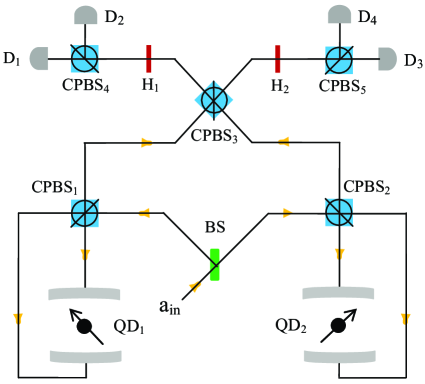
Figure 4: (Color online) Schematic diagram of the efficient PCD on the two QDs in the same node. H₁ and H₂ are two half-wave plates and each is used to complete the Hadamard rotation on the circularly polarized photons.

Suppose the two stationary spin qubits $e_{1}$ and $e_{2}$ confined in $QD_{1}$ and $QD_{2}$ are in arbitrary superposition states $|\Phi\rangle_{e_{1}}=\alpha_{1}|\uparrow\rangle+\beta_{1}|\downarrow\rangle$ and $|\Phi\rangle_{e_{2}}=\alpha_{2}|\uparrow\rangle+\beta_{2}|\downarrow\rangle$, respectively. Here $|\alpha_{1}|^{2}+|\beta_{1}|^{2}=|\alpha_{2}|^{2}+|\beta_{2}|^{2}=1$. A polarized photon p in the state $|\Phi\rangle_{p}=\frac{1}{\sqrt{2}}(|R\rangle+|L\rangle)$ input into the a_in import of the PCD (shown in Fig. 4). After passing through the BS, it is changed into the state

$$|\Phi_{1}\rangle_{p}=\frac{1}{2}(|R\rangle+|L\rangle)_{a}\otimes(|a_{1}\rangle+|a_{2}\rangle),$$ (17)

where $|a_{1}\rangle$ and $|a_{2}\rangle$ are two spatial modes of the photon a that are sent to $QD_{1}$ and $QD_{2}$, respectively. The photon in the states $|R\rangle$ and $|L\rangle$ is separated by CPBSs, and then enters the cavities. When the photon leaves the cavities, the system composed of the photon p, $e_{1}$, and $e_{2}$ evolves into the state $|\Phi_{h}\rangle_{1}$. Here

$$|\Phi_{h}\rangle_{1}\!\! = \!\!\frac{1}{2}(|R^{\uparrow}\rangle\!+\!|L^{\downarrow}\rangle)_{a}\!\otimes\![|a_{1}\rangle\!\otimes\!(\alpha_{1}|\uparrow\rangle\!-\!\beta_{1}|\downarrow\rangle)_{e_{1}}\!\otimes\!|\Phi\rangle_{e_{2}}$$ (18)

$$\!+\;|\Phi\rangle_{e_{1}}\!\otimes\!|a_{2}\rangle\!\otimes\!(\alpha_{2}|\uparrow\rangle\!-\!\beta_{2}|\downarrow\rangle)_{e_{2}}].$$

CPBS₁ and CPBS₂ are used to combine the photon in the states $|R^{\uparrow}\rangle$ and $|L^{\downarrow}\rangle$ in each spatial mode. The two spatial modes $|a_{1}\rangle$ and $|a_{2}\rangle$ of photon p interfere with each other at CPBS₃, and then a Hadamard rotation H₁ or H₂ on the photon p is applied. The state of the system composed of p, $e_{1}$, and $e_{2}$ becomes

$$|\Phi_{h}\rangle_{2}\! = \!\frac{1}{\sqrt{2}}[|R_{a_{1}}\rangle\otimes(\alpha_{1}\alpha_{2}|\uparrow,\uparrow\rangle-\beta_{1}\beta_{2}|\downarrow,\downarrow\rangle)_{e_{1}e_{2}}\!$$ (19)

$$+\;|L_{a_{1}}\rangle\otimes(\beta_{1}\alpha_{2}|\downarrow,\uparrow\rangle-\alpha_{1}\beta_{2}|\uparrow,\downarrow\rangle)_{e_{1}e_{2}}\!$$

$$+\;|R_{a_{2}}\rangle\otimes(\alpha_{1}\alpha_{2}|\uparrow,\uparrow\rangle-\beta_{1}\beta_{2}|\downarrow,\downarrow\rangle)_{e_{1}e_{2}}\!$$

$$+\;|L_{a_{2}}\rangle\otimes(\alpha_{1}\beta_{2}|\uparrow,\downarrow\rangle-\beta_{1}\alpha_{2}|\downarrow,\uparrow\rangle)_{e_{1}e_{2}}].\;\;\;\;\;\;\;\;\;$$

Here, the subscripts ${a_{1}}$ and ${a_{2}}$ represent the spatial modes of photon p sent to the left analyzer and the right one, respectively. One can project the state of the two spins nondestructively into the state

$$|\Phi^{{}_{E}}_{2}\rangle_{e}=\frac{1}{\sqrt{2}}(\alpha_{1}\alpha_{2}|\uparrow,\uparrow\rangle-\beta_{1}\beta_{2}|\downarrow,\downarrow\rangle)_{e_{1}e_{2}},$$ (20)

when a $|R\rangle$ polarized photon is detected by the single-photon detectors; otherwise, the state of the two spins will collapse into

$$|\Phi^{{}_{O}}_{2}\rangle_{e}=\frac{1}{\sqrt{2}}(\alpha_{1}\beta_{2}|\uparrow,\downarrow\rangle-\beta_{1}\alpha_{2}|\downarrow,\uparrow\rangle)_{e_{1}e_{2}}.$$ (21)

That is to say, the click of the photon detector D₁ or D₃ announces the even parity of the two spins and the click of D₂ or D₄ heralds the odd parity of the two spins.

Considering $N+1$ communication nodes, say, Alice ($e_{a}$), Bob ($e_{b}$),…, Zach ($e_{z}$) and Dean ($e_{d}$), the original $N$-electron GHZ state shared by Alice, Bob,…, and Zach is $|\Phi^{-}_{{}_{N}}\rangle_{e}=\frac{1}{\sqrt{2}}(|\!\uparrow\uparrow\dots\uparrow\rangle-|\!\downarrow\downarrow\dots\downarrow\rangle){e_{a}e_{b}\cdots{}e_{z}}$, and the Bell state shared by Zach ($e_{z^{\prime}}$) and Dean is $|\Phi^{-}_{2}\rangle_{e}=\frac{1}{\sqrt{2}}(|\!\uparrow\uparrow\rangle-|\!\downarrow\downarrow\rangle)$. The total spin state of the $N^{\prime}=N+2$ electrons can be written as

$$|\Phi_{h}\rangle_{3}\! = \!|\Phi^{-}_{{}_{N}}\rangle_{e}\otimes|\Phi^{-}_{2}\rangle_{e}$$ (22)

$$= \!\frac{1}{2}(|\uparrow,\uparrow,\dots,\uparrow\rangle-|\downarrow,\downarrow,\dots,\downarrow\rangle)_{e_{a}\cdots{}e_{z}}$$

$$\otimes\;(|\uparrow,\uparrow\rangle-|\downarrow,\downarrow\rangle)_{e_{z^{\prime}}e_{d}}.\;\;\;\;\;\;\;\;\;\;\;\;\;\;\;\;\;\;\;\;\;\;\;\;\;\;\;\;$$

If Zach applies the PCD on the two QDs $e_{z}$ and $e_{z^{\prime}}$, the system composed of the $N^{\prime}$ electrons will evolve into $|\Phi_{h}\rangle_{4}$, before the click of photon detectors in the PCD shown in Fig. 4. Here

$$|\Phi_{h}\rangle_{4}\!\! = \!\!\frac{1}{2\sqrt{2}}[(|R_{a_{1}}\rangle+|R_{a_{2}}\rangle)\otimes(|\uparrow,\cdots\uparrow,\uparrow,\uparrow\rangle$$ (23)

$$-\;|\downarrow,\cdots,\downarrow,\downarrow,\downarrow\rangle)_{e_{a}\cdots{}e_{z},e_{z^{\prime}}e_{d}}\!$$

$$+\;(|L_{a_{1}}\rangle-|L_{a_{2}}\rangle)\otimes(|\uparrow,\cdots\uparrow,\downarrow,\downarrow\rangle$$

$$-\;|\downarrow,\cdots,\downarrow,\uparrow,\uparrow\rangle)_{e_{a}\cdots{}e_{z},e_{z^{\prime}}e_{d}}],\!\;\;\;\;\;\;\;\;\;\;\;\;\;\;\;\;\;\;\;\;\;\;\;\;$$

where the $N^{\prime}$ stationary QDs are divided into the even parity case $|\Phi^{E}_{N^{\prime}}\rangle_{e}$ and the odd-parity one $|\Phi^{O}_{N^{\prime}}\rangle_{e}$ conditioned on the detection of $|R\rangle$ and $|L\rangle$ photon, respectively, i.e.,

$$|\Phi^{E}_{N^{\prime}}\rangle_{e}\!\! = \!\!\frac{1}{\sqrt{2}}(|\!\uparrow,\cdots,\uparrow,\uparrow,\uparrow\rangle\!-\!|\!\downarrow,\cdots,\downarrow,\downarrow,\downarrow\rangle)_{e_{a}\cdots{}e_{z},e_{z^{\prime}}e_{d}},$$

$$|\Phi^{O}_{N^{\prime}}\rangle_{e}\!\! = \!\!\frac{1}{\sqrt{2}}(|\!\uparrow,\cdots,\uparrow,\downarrow,\downarrow\rangle\!-\!|\!\downarrow,\cdots,\downarrow,\uparrow,\uparrow\rangle)_{e_{a}\cdots{}e_{z},e_{z^{\prime}}e_{d}}.$$

With these $N^{\prime}$-spin GHZ states, Zack performs a Hadamard operation on the two QDs $e_{z}$ and $e_{z^{\prime}}$, and then he measures the states of $e_{z}$ and $e_{z^{\prime}}$ with the basis $\{|\uparrow\rangle,|\downarrow\rangle\}$, which will project the remaining $N$ QDs $e_{a}$, $e_{b}$, $\cdots$, and $e_{d}$ into the desired GHZ state with the form $|\Phi^{-}_{{}_{N}}\rangle_{e}$, up to a local operation on $e_{d}$. The span of the GHZ quantum channel is eventually further extended. Meanwhile, if one takes another GHZ state instead of the Bell state $|\Phi^{-}_{2}\rangle_{e}$ to perform the entanglement extension, the number of the parties involved in the repeater can also be increased and the parties in the quantum communication network can, in principle, extend arbitrarily their communication distance with the same quantum entanglement extension process described above.

III Entanglement purification to depress the influence of asymmetric noise on different time bins

We have detailed the principle and the process of our heralded quantum repeater protocol, in which the influences of the noisy channels on the early and the late time bins of the photons are considered to be the same one and the fluctuation of the noise at the nanosecond scale has been neglected. In a practical condition, maybe the channel is noisy and the fiber parameters have local fast variations. The influences of the noisy channels can vary at the different time bins. The unitary transformation $U_{i}^{l}$ at the late time bin $|l\rangle$ is different from $U_{i}^{s}$ at the early time bin $|s\rangle$. At this time, the final entangled state of the two-QD subsystem will be less entangled and the entanglement purification process Qrepeater0 ; high-frep1 ; repeaterwangc is required to obtain the maximally entangled state for nonlocal electron-spin systems.

Suppose the influences of the noisy channels at the different time bins are of little difference. The unitary transformations on the early time bin and the late one are described with $U_{i}^{s}$ and $U_{i}^{l}$, respectively,

$$\begin{split}U_{i}^{s}|H\rangle_{i}\;\;=\;\;&\delta_{i}|H\rangle_{i}+\eta_{i}|V\rangle_{i},\\ U_{i}^{l}|H\rangle_{i}\;\;=\;\;&\delta^{\prime}_{i}|H\rangle_{i}+\eta^{\prime}_{i}|V\rangle_{i},\end{split}$$ (25)

where $|\delta_{i}|^{2}+|\eta_{i}|^{2}=|\delta^{\prime}_{i}|^{2}+|\eta^{\prime}_{i}|^{2}=1$ ($i=a$, $b$ ). The state of the two-photon system after passing through the noisy channels can be described as

$$|\Phi^{+}_{2}\rangle_{t_{4}}\!\!\! = \!\!\!\frac{1}{\sqrt{2}}\big{[}|s\rangle_{a}|s\rangle_{b}(\delta_{a}|H\rangle_{a}+\eta_{a}|V\rangle_{a})(\delta_{b}|H\rangle_{b}+\eta_{b}|V\rangle_{b})$$

$$\!\!\!+|l\rangle_{a}|l\rangle_{b}(\delta^{\prime}_{a}|H\rangle_{a}+\eta^{\prime}_{a}|V\rangle_{a})(\delta^{\prime}_{b}|H\rangle_{b}+\eta^{\prime}_{b}|V\rangle_{b})\big{]},\;\;\;$$

which is a partially entangled Bell state when considering the time-bin qubits but the polarization states of the photons $ab$ at different time bins are ambiguous and separable. With the same decoder in each node shown in Fig. 3 (b), the early components of the photons $ab$ will be converted into the time-bin qubits with the polarization state $|V\rangle_{a}|V\rangle_{b}$, while the late components of $ab$ will be converted into another kind of time-bin qubits with the polarization state $|H\rangle_{a}|H\rangle_{b}$ which equals to the early one only when the symmetric noise model is effective ($U_{i}^{s}=U_{i}^{l}$). After Bob performs a $\pi$ phase shift on the $|V\rangle_{b}$ component of the photon $b$, and before the photon $b$ passes through the QWPs placed near the imports of the cavities, the state of the photonic subsystem can be written as follows:

$$|\Phi^{+}_{2}\rangle_{t_{5}}\!\! = \!\!\!\frac{1}{\sqrt{2}}\big{[}-|V^{\downarrow}\rangle_{a}|V^{\downarrow}\rangle_{b}(\delta_{a}|s^{\prime}\rangle_{a}+\eta_{a}|l^{\prime}\rangle_{a})$$ (27)

$$\!\!\otimes(\delta_{b}|s^{\prime}\rangle_{b}+\eta_{b}|l^{\prime}\rangle_{b})+|H^{\uparrow}\rangle_{a}|H^{\uparrow}\rangle_{b}$$

$$\!\!\otimes(\delta^{\prime}_{a}|s^{\prime}\rangle_{a}+\eta^{\prime}_{a}|l^{\prime}\rangle_{a})(\delta^{\prime}_{b}|s^{\prime}\rangle_{b}+\eta^{\prime}_{b}|l^{\prime}\rangle_{b})\big{]},\;\;\;\;\;\;\;\;$$

which is a partially entangled polarization state when the time bin information is determined. Since the unitary transformations are arbitrary and unknown, one can describe the photonic state with the density matrix $\rho$,

$$\rho=\mu|\Phi^{-}_{2}\rangle_{0}\langle\Phi^{-}_{2}|+(1-\mu)|\Phi^{+}_{2}\rangle_{0}\langle\Phi^{+}_{2}|,$$ (28)

which can be viewed as a mixture of $|\Phi^{-}_{2}\rangle_{0}=\frac{1}{\sqrt{2}}(|H^{\uparrow}\rangle_{a}|H^{\uparrow}\rangle_{b}-|V^{\downarrow}\rangle_{a}|V^{\downarrow}\rangle_{b})$ and $|\Phi^{+}_{2}\rangle_{0}=\frac{1}{\sqrt{2}}(|H^{\uparrow}\rangle_{a}|H^{\uparrow}\rangle_{b}+|V^{\downarrow}\rangle_{a}|V^{\downarrow}\rangle_{b})$ with the probabilities $\mu$ and $1-\mu$, respectively.

We would like to consider first the case that the photons $ab$ are in the state $|\Phi^{+}_{2}\rangle_{0}$ before entering the cavities. With a similar process to that for $|\Phi^{-}_{2}\rangle_{0}$, we can complete the entanglement transfer from the photonic subsystem to the QDs subsystem, since the relative phase between different polarization modes of the photons will be mapped into the relative phase between the different spin states of the QD-confined electrons. The state of the hybrid system composed of the photons $ab$ and the electron spins $e_{a}e_{b}$ after the interactions evolves to $|\Phi^{+}_{h}\rangle$, instead of $|\Phi^{-}_{h}\rangle$ shown in Eq. (15). Here

$$|\Phi^{+}_{h}\rangle\!\!\! = \!\!\!\frac{1}{2\sqrt{2}}\big{[}(|R^{\uparrow}R^{\uparrow}\rangle\!+\!|L^{\downarrow}L^{\downarrow}\rangle)_{ab}\!\otimes\!(|\downarrow\downarrow\rangle\!+\!|\uparrow\uparrow\rangle)_{e_{a}e_{b}}$$ (29)

$$+(|R^{\uparrow}L^{\downarrow}\rangle\!+\!|L^{\downarrow}R^{\uparrow}\rangle)_{ab}\!\otimes\!(|\downarrow\uparrow\rangle\!+\!|\uparrow\downarrow\rangle)_{e_{a}e_{b}}\big{]}.\;\;\;\;\;\;\;\;$$

Comparing the hybrid state shown in Eq. (29) with that in Eq. (15), one can easily see that when the input photons are in the mixed state $\rho$, the detection of one photon in each node will project the electron spins $e_{a}e_{b}$ into another mixed state $\rho^{\prime\prime}$ with or without an additional single-qubit bit-flip operation on $e_{a}$,

$$\rho^{\prime\prime}=\mu|\Phi_{2}^{-}\rangle_{e_{0}}\langle\Phi_{2}^{-}|+(1-\mu)|\Phi_{2}^{+}\rangle_{e_{0}}\langle\Phi_{2}^{+}|.$$ (30)

It is a mixture of two-QD Bell states $|\Phi_{2}^{-}\rangle_{e_{0}}=1/\sqrt{2}(|\uparrow\uparrow\rangle-|\downarrow\downarrow\rangle)$ and $|\Phi_{2}^{+}\rangle_{e_{0}}=1/\sqrt{2}(|\uparrow\uparrow\rangle+|\downarrow\downarrow\rangle)$ with the probabilities $\mu$ and $1-\mu$, respectively.

When the parties in the quantum communication network have obtained the mixed state $\rho^{\prime\prime}$, they can use entanglement purification to increase the fidelity of the entangled channel between Alice and Bob. Since the phase-flip error cannot be purified directly, the parties can perform a Hadamard operation on each QD and convert the joint state of $e_{a}$ and $e_{b}$ into

$$\rho^{\prime\prime}_{h}=\mu|\Phi_{0}^{{}^{\prime}-}\rangle_{e}\langle\Phi_{0}^{{}^{\prime}-}|+(1-\mu)|\Phi_{0}^{{}^{\prime}+}\rangle_{e}\langle\Phi_{0}^{{}^{\prime}+}|.$$ (31)

Here $|\Phi_{0}^{{}^{\prime}-}\rangle_{e}\!=\frac{1}{\sqrt{2}}(|\uparrow\downarrow\rangle+|\downarrow\uparrow\rangle)$ and $|\Phi_{0}^{{}^{\prime}+}\rangle_{e}=\frac{1}{\sqrt{2}}(|\uparrow\uparrow\rangle+|\downarrow\downarrow\rangle)$. The original phase-flip error is mapped into a bit-flip error, and Alice and Bob can perform the entanglement purification process with our efficient PCD to improve the fidelity of the mixed state $\rho^{\prime\prime}_{h}$. Its principle can be described in detail as follows.

Alice and Bob can take two copies of QD systems $e_{a}e_{b}$ and $e^{\prime}_{a}e^{\prime}_{b}$ for each round of purification and each system is in the state $\rho^{\prime\prime}_{h}$. The composite four-QD system is in the state $\rho_{P}^{T}$ which could be viewed as the mixture of four pure states $|\Phi_{0}^{{}^{\prime}-}\rangle_{e_{a}e_{b}}\otimes|\Phi_{0}^{{}^{\prime}-}\rangle_{e_{a}^{{}^{\prime}}e_{b}^{{}^{\prime}}}$, $|\Phi_{0}^{{}^{\prime}-}\rangle_{e_{a}e_{b}}\otimes|\Phi_{0}^{{}^{\prime}+}\rangle_{e_{a}^{{}^{\prime}}e_{b}^{{}^{\prime}}}$, $|\Phi_{0}^{{}^{\prime}+}\rangle_{e_{a}e_{b}}\otimes|\Phi_{0}^{{}^{\prime}-}\rangle_{e_{a}^{{}^{\prime}}e_{b}^{{}^{\prime}}}$, and $|\Phi_{0}^{{}^{\prime}+}\rangle_{e_{a}e_{b}}\otimes|\Phi_{0}^{{}^{\prime}+}\rangle_{e_{a}^{{}^{\prime}}e_{b}^{{}^{\prime}}}$ with the probabilities of $\mu^{2}$, $\mu(1-\mu)$, $\mu(1-\mu)$, and $(1-\mu)^{2}$, respectively. After the PCDs performed by Alice and Bob, if all the outcomes are even, the total four-QD system $e_{a}e_{b}e^{\prime}_{a}e^{\prime}_{b}$ will be projected into the state,

$$|\varphi\rangle=\frac{1}{\sqrt{2}}(|\uparrow\downarrow\uparrow\downarrow\rangle\!+\!|\downarrow\uparrow\downarrow\uparrow\rangle)_{e_{a}e_{b}e^{\prime}_{a}e^{\prime}_{b}},$$ (32)

with the probability of $\frac{\mu^{2}}{2}$ and

$$|\varphi^{{}^{\prime}}\rangle=\frac{1}{\sqrt{2}}(|\uparrow\uparrow\uparrow\uparrow\rangle\!+\!|\downarrow\downarrow\downarrow\downarrow\rangle)_{e_{a}e_{b}e^{\prime}_{a}e^{\prime}_{b}},$$ (33)

with the probability of $\frac{(1-\mu)^{2}}{2}$, respectively. If both Alice and Bob get an odd-parity result, they perform a bit-flip operation on their electron spins $e_{a}$ and $e_{b}$, which leads to the same projection of the QD system as the case that both outcomes of the two PCDs are even. As for the case with one odd parity and one even parity, which originates from the cross state $|\Phi_{0}^{{}^{\prime}+}\rangle_{e_{a}e_{b}}\otimes|\Phi_{0}^{{}^{\prime}-}\rangle_{e_{a}^{{}^{\prime}}e_{b}^{{}^{\prime}}}$ and $|\Phi_{0}^{{}^{\prime}-}\rangle_{e_{a}e_{b}}\otimes|\Phi_{0}^{{}^{\prime}+}\rangle_{e_{a}^{{}^{\prime}}e_{b}^{{}^{\prime}}}$, it leads to the error and should be discarded. In other words, with the PCDs, Alice and Bob can project the QD system $e_{a}e_{b}e_{a}^{{}^{\prime}}e_{b}^{{}^{\prime}}$ into

$$\rho^{\prime\prime}_{h_{1}}\!=\!\frac{\mu^{2}}{\mu^{2}+(1-\mu)^{2}}|\varphi\rangle\langle\varphi|\!+\!\frac{(1-\mu)^{2}}{\mu^{2}\!+\!(1-\mu)^{2}}|\varphi^{{}^{\prime}}\rangle\langle\varphi^{{}^{\prime}}|,\;\;\;\;$$ (34)

with the probability of ${\mu^{2}+(1-\mu)^{2}}$, when their outcomes are the same ones in their PCD processes.

In order to obtain the entangled state of a two-QD subsystem $e^{\prime}_{a}e^{\prime}_{b}$, both Alice and Bob perform a Hadamard operation on their electron spins $e_{a}$ and $e_{b}$. By measuring the spin states of the QDs $e_{a}$ and $e_{b}$ with the basis $\sigma_{z}=\{|\uparrow\rangle,\,|\downarrow\rangle\}$, they can, with or without some phase-flip operations, get the desired QD subsystem $e^{\prime}_{a}e^{\prime}_{b}$ in the states $|\Phi^{{}^{\prime}-}_{0}\rangle_{e}$ and $|\Phi^{{}^{\prime}+}_{0}\rangle_{e}$ with the probabilities of $\frac{\mu^{2}}{\mu^{2}+(1-\mu)^{2}}$ and $\frac{(1-\mu)^{2}}{\mu^{2}+(1-\mu)^{2}}$, respectively. Finally, another Hadamard operation on $e^{\prime}_{a}$ and $e^{\prime}_{b}$ will convert the states $|\Phi^{{}^{\prime}-}_{0}\rangle_{e}$ and $|\Phi^{{}^{\prime}+}_{0}\rangle_{e}$ back into $|\Phi_{2}^{-}\rangle_{e_{0}}$ and $|\Phi_{2}^{+}\rangle_{e_{0}}$, respectively, leaving the whole system in the state,

$$\rho_{f}^{\prime\prime}\!=\!\frac{\mu^{2}}{\mu^{2}\!+\!(1\!-\!\mu)^{2}}|\Phi_{2}^{-}\rangle_{e_{0}}\langle\Phi_{2}^{-}|\!+\!\frac{(1\!-\!\mu)^{2}}{\mu^{2}\!+\!(1\!-\!\mu)^{2}}|\Phi_{2}^{+}\rangle_{e_{0}}\langle\Phi_{2}^{+}|.$$

It is a mixed entangled state with a higher fidelity than that in the original one $\rho^{\prime\prime}$ when $\mu>1/2$.

Certainly, the parties can improve further the fidelity of the nonlocal quantum systems by iterating the purification protocol several rounds with the method described above. For instance, if the initial state with the fidelity $\mu>0.7$ is available, they can achieve the state with the fidelity $F>0.997$ for only two rounds.

IV Influence on fidelity and efficiency from the practical circular birefringence

In the discussion above, the spin-selection rule is taken to be perfect and $2g^{2}/\kappa\gamma\gg 1$, and the resonant condition $|\Delta|\simeq 0$ is satisfied. In fact, the heavy-light hole mixing can reduce the fidelity of the optical selection rules hole-mixing , and it can be improved for charged excitons due to the quenched exchanged interaction hole-mixings . Meanwhile, the finite linewidth of the input light pulse will inevitably make the resonant condition diffusion. The side leakage of the cavity $\kappa_{s}$ and the limited coupling strength $g$ will lead to the imperfect birefringent propagation of the input photons Qdcoupling3 ; Qdcoupling4 as well. For instance, when the electron spin is in the spin-up state $|\uparrow\rangle$, the incident photon $|R^{\uparrow}\rangle$ or $|L^{\downarrow}\rangle$ totally reflected in the ideal case has a probability $t$ to be transmitted through the cavity, and $|L^{\uparrow}\rangle$ or $|R^{\downarrow}\rangle$ supposed to be totally transmitted has a probability $r_{0}$ to be reflected.

To discuss the influence of the imperfect circular birefringence for the QD-cavity unit on the fidelity of the quantum distribution process, let us take the entanglement distribution with the symmetric noise model as an example. In this case, the photons $a$ and $b$ input into the cavities are in the state $|\Phi^{-}_{2}\rangle_{c}=(|R^{\uparrow},R^{\uparrow}\rangle-|L^{\downarrow},L^{\downarrow})/\sqrt{2}$, and the QD-confined electron spins $e_{i}$ ($i=a,b$) are all initialized to the state $|\Phi\rangle_{e_{i}}=\frac{1}{\sqrt{2}}(|\uparrow\rangle+|\downarrow\rangle)$. The simplified transformation relationship described in Eqs. (7) and (8) for an ideal QD-cavity unit should be modified, and the original transformation in Eq. (4) becomes dominant. When the electron spin is in the spin-up state $|\uparrow\rangle$, one has the following transformations:

$$\begin{split}|R^{\uparrow},\uparrow\rangle\;\;\rightarrow\;\;&r|L^{\downarrow},\uparrow\rangle+t|R^{\uparrow},\uparrow\rangle,\\ |R^{\downarrow},\uparrow\rangle\;\;\rightarrow\;\;&t_{0}|R^{\downarrow},\uparrow\rangle+r_{0}|L^{\uparrow},\uparrow\rangle,\\ |L^{\downarrow},\uparrow\rangle\;\;\rightarrow\;\;&r|R^{\uparrow},\uparrow\rangle+t|L^{\downarrow},\uparrow\rangle,\\ |L^{\uparrow},\uparrow\rangle\;\;\rightarrow\;\;&t_{0}|L^{\uparrow},\uparrow\rangle+r_{0}|R^{\downarrow},\uparrow\rangle,\end{split}$$ (36)

where $r$ ($t$ ) and $r_{0}$ ($t_{0}$) are the reflection (transmission) coefficients shown in Eqs. (5) and (6), respectively. In other words, the incident circularly polarized photon $|R^{\uparrow}\rangle$ or $|L^{\downarrow}\rangle$ totally reflected in the ideal case has a probability $t$ to be transmitted through the cavity, and $|L^{\uparrow}\rangle$ or $|R^{\downarrow}\rangle$ supposed to be totally transmitted has a probability $r_{0}$ to be reflected. When the excess electron is in the state $|\downarrow\rangle$, the evolution can be described similarly as:

$$\begin{split}|R^{\uparrow},\downarrow\rangle\;\;\rightarrow\;\;&t_{0}|R^{\uparrow},\downarrow\rangle+r_{0}|L^{\downarrow},\downarrow\rangle,\\ |R^{\downarrow},\downarrow\rangle\;\;\rightarrow\;\;&r|L^{\uparrow},\downarrow\rangle+t|R^{\downarrow},\downarrow\rangle,\\ |L^{\uparrow},\downarrow\rangle\;\;\rightarrow\;\;&r|R^{\downarrow},\downarrow\rangle+t|L^{\uparrow},\downarrow\rangle,\\ |L^{\downarrow},\downarrow\rangle\;\;\rightarrow\;\;&t_{0}|L^{\downarrow},\downarrow\rangle+r_{0}|R^{\uparrow},\downarrow\rangle.\end{split}$$ (37)

According to the practical transformations in Eqs. (36) and (37), the non-normalized state of the composite hybrid photon-QD system after the reflection of the photons $ab$ can be written as

$$|\Phi^{-^{\prime}}_{h}\rangle\!\! = \!\!\!\frac{1}{2\sqrt{2}}\Big{\{}(|R^{\uparrow},R^{\uparrow}\rangle-|L^{\downarrow},L^{\downarrow}\rangle)\big{[}(t^{2}-r^{2})|\uparrow\uparrow\rangle$$ (38)

$$+(r_{0}^{2}-t_{0}^{2})|\downarrow\downarrow\rangle+(tt_{0}-rr_{0})(|\uparrow\downarrow\rangle+|\downarrow\uparrow\rangle)\big{]}$$

$$+(rt_{0}-tr_{0})(|R^{\uparrow},L^{\downarrow}\rangle-|L^{\downarrow},R^{\uparrow}\rangle)$$

$$\otimes(|\uparrow\downarrow\rangle+|\downarrow\uparrow\rangle)\Big{\}}.$$

Conditioned on the click of one single-photon detector at each side, the entanglement distribution process is supposed to be completed, and the electron spins $e_{a}e_{b}$ will be collapsed into two different partially entangled states depending on the outcomes of photon detections.

To be detailed, when the outcomes of the measurements on photons $ab$ result in the even-parity space $S=\{|R^{\uparrow},R^{\uparrow}\rangle,|L^{\downarrow},L^{\downarrow}\rangle\}$, the electron spins $e_{a}e_{b}$ will be projected into the following state:

$$|\Phi^{-^{\prime}}_{2}\rangle_{e}\!\! = \!\!\!\frac{1}{2\sqrt{2}}\big{[}(t^{2}-r^{2})|\uparrow\uparrow\rangle+(r_{0}^{2}-t_{0}^{2})|\downarrow\downarrow\rangle$$ (39)

$$+(tt_{0}-rr_{0})(|\uparrow\downarrow\rangle+|\downarrow\uparrow\rangle)\big{]},$$

with a success probability,

$$\eta_{d}^{{}_{E}}=\frac{|2t+1|^{2}+|2t_{0}+1|^{2}+2|1+t+t_{0}|^{2}}{4}.$$ (40)

Note $r\equiv 1+t$ and $r_{0}\equiv 1+t_{0}$ as shown in Eqs. (5) and (6). Therefore, the fidelity $F^{{}_{E}}_{d}$ of the heralded entanglement between the electron spins $e_{a}e_{b}$ compared with the ideal target state $|\Phi^{-}_{2}\rangle_{e}$ of entanglement distribution obtained with the perfect birefringence in this case, can be detailed as

$$F^{{}_{E}}_{d} = \big{|}{}_{e}\langle\Phi^{-}_{2}|\Phi^{-^{\prime}}_{2}\rangle_{e}\big{|}^{2}$$ (41)

$$= \frac{|t^{2}-r^{2}-t_{0}^{2}+r_{0}^{2}|^{2}}{2(|t^{2}-r^{2}|^{2}+|r_{0}^{2}-t_{0}^{2}|^{2}+2|tt_{0}-rr_{0}|^{2})}$$

$$= \frac{|t_{0}-t|^{2}}{2\eta_{d}^{{}_{E}}}.$$

In the other case, when the outcomes of photon detections belong to the odd-parity space $AS=\{|R^{\uparrow},L^{\downarrow}\rangle,|L^{\downarrow},R^{\uparrow}\rangle\}$, the hybrid photon-QD in state $|\Phi^{-^{\prime}}_{h}\rangle$ collapses the electron spins $e_{a}e_{b}$ into the state,

$$|\Phi^{-^{\prime}}_{2}\rangle_{a} = \frac{1}{\sqrt{2}}(|\uparrow\downarrow\rangle-|\downarrow\uparrow\rangle),$$ (42)

with a probability of

$$\eta_{d}^{{}_{O}}=\frac{|t_{0}-t|^{2}}{2}.$$ (43)

After Bob performs the bit-flip operation $\sigma^{b}_{x}=|\uparrow\rangle\langle\downarrow|+|\downarrow\rangle\langle\uparrow|$ on the electron spin $e_{b}$, the same as the case that the perfect circular birefringence is effective, the state of the two electrons $e_{a}e_{b}$ evolves into

$$|\Phi^{-^{\prime}}_{2}\rangle_{b} = \frac{1}{\sqrt{2}}(|\uparrow\uparrow\rangle-|\downarrow\downarrow\rangle),$$ (44)

which is the practical state of the electron spins $e_{a}e_{b}$ after the entanglement distribution, and it is identical to the target state $|\Phi^{-}_{2}\rangle_{e}$. In other words, the fidelity $F^{{}_{O}}_{d}$ for this case is unity,

$$F^{{}_{O}}_{d}=1,$$ (45)

which is independent of both the coupling strength $g/\kappa$ and the cavity leakage $\kappa_{s}/\kappa$, and the corresponding efficiency equals to $\eta^{{}_{O}}_{d}$.

From the discussion above, one can see that after entanglement distribution the state of the electron spins $e_{a}e_{b}$ depends on the outcomes of the photon detection as a result of the imperfect birefringent propagation of photons. That is, $|\Phi^{-^{\prime}}_{2}\rangle_{e}$ and $|\Phi^{-^{\prime}}_{2}\rangle_{b}$ are conditioned on the outcomes of photon detection in $S$ and $AS$, respectively. Therefore, the total efficiency of the entanglement distribution can be detailed as

$$\eta_{d}=\eta_{d}^{{}_{O}}+\eta_{d}^{{}_{E}}=\frac{{|2t+1|^{2}+|2t_{0}+1|^{2}}}{2},$$ (46)

shown in Fig. 5 (a). Meanwhile, the fidelities $F^{{}_{E}}_{d}$ and $F^{{}_{O}}_{d}$ measure the overlap between the ideal target state $|\Phi^{-}_{2}\rangle_{e}$ and the practical states $|\Phi^{-^{\prime}}_{2}\rangle_{e}$ and that between $|\Phi^{-}_{2}\rangle_{e}$ and $|\Phi^{-^{\prime}}_{2}\rangle_{b}$, respectively. When the input maximally entangled state of $ab$ is $|\Phi_{2}^{-}\rangle_{c}=1/\sqrt{2}(|R^{\uparrow},R^{\uparrow}\rangle-|L^{\downarrow},L^{\downarrow})_{ab}$, the ideal target state $|\Phi^{-}_{2}\rangle_{e}$ of $e_{a}e_{b}$ is fully orthogonal to the original state of the two-electron system that equals the practical one when spins $e_{a}e_{b}$ does not interact with the photons, which leads to the vanish fidelity $F^{{}_{E}}_{d}=0$ for the outcome of the photon detection in $S$ when the coupling strength $g/\kappa=0$. However, when the outcome of the photon detection is in $AS$, we can get the unity fidelity $F^{{}_{O}}_{d}$ for entanglement distribution, even with the imperfect input-output process, since the imperfect birefringence of the QD-cavity system will appear as a whole coefficient; see Eq. (39) for detail. However, for $g=0$, the corresponding efficiency $\eta_{d}^{{}_{O}}$ for the outcome in $AS$ of the photon detection in entanglement distribution vanishes $(\eta_{d}^{{}_{O}}=0)$, shown in Fig. 5(b).

During the entanglement extension process, the party utilizes a PCD on two local spin qubits, and performs the partial measurements on the spins. The influence of the practical circular birefringence on the entanglement extension process can be estimated by the performance of the PCD when the two QDs are in the state $|\Phi\rangle_{ee^{\prime}}=\frac{1}{2}(|\uparrow\uparrow\rangle+|\downarrow\uparrow\rangle+|\uparrow\downarrow\rangle+|\downarrow\downarrow\rangle)_{ee^{\prime}}$. The state of the composite hybrid system composed of the input probe photon p and the electron spin $ee^{\prime}$ before the detection on the photon p evolves into

$$|\Phi_{h}^{\prime}\rangle_{1}\!\! = \!\!\frac{1}{4\sqrt{2}}\Big{\{}(|R_{1}\rangle+|R_{2}\rangle)[2(r+t)|\uparrow\uparrow\rangle+2(r_{0}+t_{0})$$

$$\times|\downarrow\downarrow\rangle+(r+t+r_{0}+t_{0})(|\uparrow\downarrow\rangle+|\downarrow\uparrow\rangle)]$$

$$+(|L_{2}\rangle-|L_{1}\rangle)(r+t-r_{0}-t_{0})(|\uparrow\downarrow\rangle-|\downarrow\uparrow\rangle)\Big{\}},$$

and the corresponding success probability $\eta_{p}$ can be detailed as

$$\eta_{p}=\eta_{p}^{{}_{O}}+\eta_{p}^{{}_{E}}=\frac{|2t+1|^{2}+|2t_{0}+1|^{2}}{2},$$ (48)

which is identical to that for entanglement distribution $\eta_{d}$, and it equals to the efficiency of the entanglement extension when the single-qubit operation and the detection of the QD electron spins are perfect qqtime4 ; opticalpum1 ; opticalpum2 ; rotation ; time1 . Here, $\eta_{p}^{{}_{O}}=\eta_{d}^{{}_{O}}=(|t-t_{0}|^{2})/2$ and $\eta_{p}^{{}_{E}}=\eta_{d}^{{}_{E}}=({|2t+1|^{2}+|2t_{0}+1|^{2}+2|1+t+t_{0}|^{2}})/{4}$ represent the probabilities for the heralded success of the entanglement extension by detecting an $|L\rangle$ (odd parity of the PCD for two spins in the ideal case) and a $|R\rangle$ (even parity of the PCD for two spins in the ideal case) polarized photons, respectively. When $g/\kappa=0$, it leads to $\eta_{p}^{{}_{O}}=0$ no matter whether $\kappa_{s}=0$ or not, since the probe photon in state $|\Phi\rangle_{p}=(|R\rangle+|L\rangle)/\sqrt{2}$ does not interact with the QDs and it is still in the state $|\Phi\rangle_{p}$ when it interferes with itself at CPBS₃, shown in Fig. 4. This photon will be transformed into the $|R\rangle$ polarized photon by the Hadamard operation $H_{1}$ or $H_{2}$ and it never leads to the click of detectors $D_{2}$ or $D_{4}$, shown in Fig. 4.

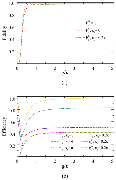
Figure 5: (Color online) The performance of entanglement distribution. (a) The fidelities $F^{O}_{d}$ and $F^{E}_{d}$ conditioned on different outcomes of photon detection in the entanglement distribution vs the normalized coupling strength $g/\kappa$. (b) The efficiency $\eta_{d}$ of entanglement distribution vs the normalized coupling strength $g/\kappa$. Here $\eta_{d}=\eta^{{}_{O}}_{d}+\eta^{{}_{E}}_{d}$, ${\gamma}/{\kappa}=0.1$, and the resonant condition $\omega_{c}=\omega_{X^{-}}=\omega_{0}$ is adopted.

To be detailed, when a $|R\rangle$ polarized photon is detected either in the $|R_{1}\rangle$ or $|R_{2}\rangle$ mode, the QD subsystem $ee^{\prime}$ will be collapsed into

$$|\Phi^{{}_{E^{\prime}}}_{2}\rangle_{e}\!\! = \!\!\frac{1}{2\sqrt{2}}\Big{[}2(r+t)|\uparrow\uparrow\rangle+2(r_{0}+t_{0})|\downarrow\downarrow\rangle$$ (49)

$$+(r+t+r_{0}+t_{0})(|\uparrow\downarrow\rangle+|\downarrow\uparrow\rangle)\Big{]}.\;\;\;\;\;\;\;$$

The fidelity $F^{{}_{E}}_{p}$ of the PCD with respect to the ideal even-parity output state $|\Phi_{2}^{{}_{E}}\rangle_{e}=\frac{1}{\sqrt{2}}(|\uparrow\uparrow\rangle-|\downarrow\downarrow\rangle)_{ee^{\prime}}$, obtained from Eq. (20) for $\alpha_{1}=\alpha_{2}=\beta_{1}=\beta_{2}=1/\sqrt{2}$, can be detailed as

$$F^{{}_{E}}_{p} = \big{|}{}_{e}\langle\Phi_{2}^{{}_{E}}|\Phi_{2}^{{}_{E^{\prime}}}\rangle_{e}\big{|}^{2}$$ (50)

$$= \frac{|r+t-r_{0}-t_{0}|^{2}}{2|r+t|^{2}+|r+t+r_{0}+t_{0}|^{2}+2|r_{0}+t_{0}|^{2}}$$

$$= \frac{|t_{0}-t|^{2}}{\eta^{{}_{E}}_{p}},$$

which is identical to the fidelity $F^{{}_{E}}_{d}$ with the even-parity outcome during the entanglement distribution process. For $g/\kappa=0$, the QDs $ee^{\prime}$ will be kept in the initial state $|\Phi\rangle_{ee^{\prime}}=1/2(|\uparrow\uparrow\rangle+|\downarrow\uparrow\rangle+|\uparrow\downarrow\rangle+|\downarrow\downarrow\rangle)$, which is fully orthogonal to the ideal output state $|\Phi_{0}\rangle_{ee^{\prime}}=1/\sqrt{2}(|\uparrow\uparrow\rangle-|\downarrow\downarrow\rangle)$, leading to $F^{{}_{E}}_{p}=0$. In contrast, when an $|L\rangle$ polarized photon is detected, the QD subsystem $ee^{\prime}$ will be projected into the state,

$$|\Phi^{{}_{O^{\prime}}}_{2}\rangle_{e}\!\! = \!\!\frac{1}{\sqrt{2}}\big{(}|\uparrow\downarrow\rangle-|\downarrow\uparrow\rangle\big{)},$$ (51)

which is identical to the ideal odd-parity output state $|\Phi_{2}^{{}_{O}}\rangle_{e}=\frac{1}{\sqrt{2}}(|\uparrow\downarrow\rangle-|\downarrow\uparrow\rangle)_{ee^{\prime}}$ obtained from Eq. (21) with perfect birefringent propagation when applying our PCD. Now, the fidelity $F^{{}_{O}}_{p}$ of the state $|\Phi^{{}_{O^{\prime}}}_{2}\rangle_{e}$ can be written as follows:

$$F^{{}_{O}}_{p}=1.$$ (52)

The reason is that the photon detection and the interference of the probe photon from different pathes transform the imperfect birefringence into a nonlocal coefficient; see Eq. (LABEL:praext) for detail. When $g/\kappa=0$, the nonlocal coefficient will vanish, which results in the fact that the corresponding probability $\eta_{p}^{{}_{O}}=0$.

The fidelities $F^{{}_{O}}_{d}$ and $F^{{}_{E}}_{d}$ conditioned on different outcomes of the photon detection in the entanglement distribution are shown in Fig. 5 (a) as the function of the side leakage of the spin-cavity system $\kappa_{s}/\kappa$ and the coupling strength $g/\kappa$ on the resonant interaction condition, where ${\gamma/\kappa}=0.1$ and $\omega_{c}=\omega_{X^{-}}=\omega$. Meanwhile, the fidelities $F^{{}_{O}}_{p}$ and $F^{{}_{E}}_{p}$ in entanglement extension are identical to $F^{{}_{O}}_{d}$ and $F^{{}_{E}}_{d}$, respectively. When the coupling strength $g/\kappa>0.6$ , both the entanglement distribution process and the entanglement extension process are near perfect, with the minimal fidelity $F^{{}_{E}}_{d}=F^{{}_{E}}_{p}>0.948$ for both cases with the side leakage $\kappa_{s}/\kappa=0$ and $\kappa_{s}/\kappa=0.2$. When the coupling strength $g/\kappa=1.2$, the minimum fidelities of the entanglement distribution and extension with the side leakage $\kappa_{s}/\kappa=0.2$ are $F^{{}_{E}}_{d}=F^{{}_{E}}_{p}=0.991$. They can be increased to be $F^{{}_{E}}_{d}=F^{{}_{E}}_{p}=0.998$ when $\kappa_{s}/\kappa=0$ and $g/\kappa=1.2$. Interestingly, the detection of an $|L\rangle$ polarized photon in entanglement extension and that of $|R^{\uparrow}R^{\uparrow}\rangle$ or $|L^{\downarrow}L^{\downarrow}\rangle$ in entanglement distribution can lead to the corresponding error-free processes, no matter what the coupling strength $g/\kappa$ and the side leakage $\kappa_{s}/\kappa$ are, and it is useful for generating entangled states and scalable one-way quantum computation qqentangle1 .

The total efficiency of entanglement distribution $\eta_{d}=\eta^{{}_{O}}_{d}+\eta^{{}_{E}}_{d}$ is shown in Fig. 5 (b) with the same parameters as those for the fidelities. Meanwhile, the efficiencies $\eta^{{}_{O}}_{p}$ and $\eta^{{}_{E}}_{p}$ in entanglement extension are identical to the corresponding ones $\eta^{{}_{O}}_{d}$ and $\eta^{{}_{E}}_{d}$ in entanglement distribution. One should note that when the coupling rate $g$ is small, especially, $g/\kappa<0.6$, the fidelities $F_{d}^{{}_{E}}$ and $F_{p}^{{}_{E}}$ are much smaller than $F_{d}^{{}_{O}}=F_{p}^{{}_{O}}=1$, and we should treat these two kinds of outcomes in entanglement distribution ($AS$ or $S$) and entanglement extension ($|R\rangle$ or $|L\rangle$) independently. However, when $g$ is large, the total efficiencies are more important, since both kinds of outcomes are faithful, shown in Fig. 5 (a). When the coupling strength $g/\kappa=1.2$, the efficiencies $\eta_{d}=\eta_{p}=0.770$ for the side leakage $\kappa_{s}/\kappa=0.2$. If $g/\kappa=2.4$ and $\kappa_{s}/\kappa=0$, the efficiencies $\eta_{d}=\eta_{p}=0.983$ are achievable. The small reduction from unity probability for $\kappa_{s}=0$ originates from the noise operator $(\hat{N})$ associated with the spontaneous decay of the trion state. Meanwhile, when we increase the side leakage to $\kappa_{s}=0.2\kappa$, both $\eta_{d}^{{}_{E}}$ ($\eta_{p}^{{}_{E}}$) and $\eta_{d}^{{}_{O}}$ ($\eta_{p}^{{}_{O}}$) decrease a little leading to the decrease in the total efficiency $\eta_{d}$ ($\eta_{p}$), due to the finite reflection originating from the coupling to side leakage mode $\hat{s}_{in}$. The efficiency $\eta_{d}$ ($\eta_{p}$) decreases scince the increase of the side leakage $\kappa_{s}/\kappa$ will decrease the radiation into the cavity, resulting in a decrease of the output photon in the subspace spanned by the transmission and reflection modes, shown in Fig. 2 (b). In addition, when the achievable input-coupling efficiency $\eta_{in}=90\%$ is considered q215 , the efficiencies above should be further reduced by $19\%$ and $10\%$ for the efficiencies $\eta_{d}$ and $\eta_{p}$, since two input-output processes is involved in the entanglement distribution process while only one is involved in the entanglement extension process with our efficient PCD.

V Discussion and summary

Thus far, we have detailed the process of establishing the quantum entangled channel for the quantum communication network. The photons entangled in the time-bin DOF are exploited to entangle the remotely separated QD-cavity units. Currently, the sources producing photon pairs with polarization entanglement are well developed. With some optical elements, the polarized entanglement can be transformed into the time-bin one before the transmission over noisy optical-fiber channels, shown in Fig. 3. Along with our effective PCD, the parties can perform the heralded extension of the entanglement across the quantum network with quantum swapping, and increase the entanglement with entanglement purification. In addition, by picking out the outcome of the PCD in which an $|L\rangle$ polarized photon is detected for the success signal, the two QDs will be projected into the odd-parity state in a heralded way and the influence of imperfect birefringence on the entanglement purification and the entanglement extension processes can be eliminated.

In our protocol, the electron spin of the QD acts as a quantum node. Before the arrival of the incident photon, the users initialize their spins by optical pumping or optical cooling opticalpum1 ; opticalpum2 , followed by single-spin rotations rotation ; qqtime4 . The time needed for the coherent control of electron spins has been suppressed into the scale of picosecond in the semiconductor quantum dot time1 . Meanwhile, an electron-spin coherence time as high as $T_{2}\simeq 2.6$ $\mu{}$s has been experimentally achieved timec , which is quite long compared with preparation and measurement time (ns scales). Hence, the cavity photon time $\tau=4.5$ ns will be the dominant time interval for the exciton dephasing Qdcoupling4 . The previous fidelity of the final quantum networking will be reduced by the amount of $[1-exp(-\tau/T_{2})\simeq 0.002]$. When the absence of nuclear spins is achieved, e.g., by using isotopically purified II-VI materials, the decoherence time is theoretically predicted to be as long as the spin relaxation time which is currently $20$ ms at a magnetic field $4T$ and at $1K$ qqtime2 and can be much longer for a lower magnetic field qqtime4 ; qqtime3 .

Our scheme prefers the strong coupling between the QDs and the cavity, and it can also be performed with low-$Q$-factor cavities where $g/\kappa<1$ at the price of decreasing the efficiency a bit. The strong coupling has been observed in various QD-cavity systems strongp ; strongcry . For micropillars with the diameter $d_{c}$ around 1.5 $\mu{}$m, the $X^{-}$ dipole decay rate $\gamma/2\simeq 1$ $\mu{}$eV when the temperature $T=2K$ QD-tem . The coupling strength $g=80$ $\mu{}$eV and the cavity quality factor including the side leakage as high as $Q>4\times 10^{4}$ has been experimentally realized with $In_{0.6}Ga_{0.4}As$ in a similar experiment setup q4 . In other words, $g/(\kappa+\kappa_{s})>2.4$ is achievable. Meanwhile, the coupling strength $g$ depends on the QD exciton oscillator strength and the mode volume $V$, while $\kappa$ is determined by the cavity quality factor, and they can, in principle, be controlled independently to achieve a larger $g/(\kappa+\kappa_{s})$. Recently, the coupling strength $g=16$ $\mu{}$eV and a cavity spectral width as low as $\kappa=20.5$ $\mu{}$eV ($Q$=65 000) have been achieved in a 7.3 $\mu{}$m diameter micropillar q65 . And then, the quality factor is improved to $Q=2.15\times 10^{5}$($\kappa=6.2$ $\mu{}$eV) with lower side leakage q215 .

The imperfection that comes from photon loss is also an inevitable problem in the previous schemes high-frep1 ; high-frep2 ; revqr ; ionqr ; Qdqr1 ; Qdqr2 . The photon loss occurs due to the cavity imperfection, the fiber absorption, and the inefficiency of the single-photon detector. As the successful generation of the electron-spin entangled state and the completion of quantum extension are heralded by the detection of photons, the photon loss will only affect the efficiency of our scheme and has no effect on the fidelity of the quantum channel established. During the transmission of the photons, there is no restriction on the electron spins. That is, if the photons can arrive at the nodes, the distance of the adjacent nodes can be long, different from those limited by the coherent time of the quantum nodes Qrepeater0 ; revqr as the entanglement between neighboring nodes are constructed by entanglement swapping between the stationary qubit and the flying qubit in the latter. The efficiency of our entanglement distribution protocol is at least two times more than those performed with two-photon coincidence detection Qdqr2 ; qqentangle2 , since the photonic entanglement can be totally converted into the QD entanglement conditioned on the detection of one photon at each node. Meanwhile, the multi-mode speed-up procedure QRmulti-spatial agrees with our protocol and can be involved in a similar way to that presented by Jones et al qqentangle2 .

In summary, we have proposed an efficient quantum repeater protocol for spin-photon systems with the help of the time-bin encoder and the generalized interface between the circularly polarized photon and the QD embedded in a double-sided optical microcavity. It works in a heralded way and requires only one channel, not two or more Qdqr3 . The users can establish a maximally entangled quantum channel which is independent of the particular parameters of the collective-noise channel. We also construct an efficient PCD based on one effective input-output process of a single photon, and it can simplify the entanglement channel extension and entanglement purification that is used to suppress the phase-flip errors originating from the imperfection of the collective-noise channel. This protocol is feasible with current technology and can find its application directly in the quantum communication network protocols.

Appendix A $N$-user GHZ state distribution for a multiuser quantum repeater network

The principle of our deterministic entanglement creation for two legitimate participants can be extended to the $N$-participant case directly. Assume the original local $N$-photon GHZ state in the polarization DOF can be described as

$$|\Phi^{+}_{N}\rangle=\frac{1}{\sqrt{2}}(|H\rangle_{a}|H\rangle_{b}\dots|H\rangle_{z}+|V\rangle_{a}|V\rangle_{b}\dots|V\rangle_{z}),\;\;\;$$ (53)

where the subscripts $a$, $b$, $\dots$, and $z$ represent the photons directed to Alice, Bob, $\dots$, and Zach, respectively. After a similar encoder to that in the two-photon case performed on each of the $N$ photons, the state of the system composed of the $N$ photons $ab\dots z$ launched into the noisy quantum channels becomes

$$|\Phi^{+}_{N}\rangle_{t_{0}}\!\! = \!\!\frac{1}{\sqrt{2}}|H\rangle_{a}|H\rangle_{b}\dots|H\rangle_{z}\otimes(|s\rangle_{a}|s\rangle_{b}\dots|s\rangle_{z}$$ (54)

$$+|l\rangle_{a}|l\rangle_{b}\dots|l\rangle_{z}).\;\;\;\;\;\;\;\;\;\;\;\;\;\;\;\;\;\;\;\;\;\;\;\;\;\;\;\;\;\;\;\;\;\;\;\;\;\;\;\;$$

It is an $N$-qubit time-bin entanglement. Here $|s\rangle_{i}$ and $|l\rangle_{i}$ ($i=$ $a$, $b$, $\dots$, $z$) denote the components of the photon $i$ which pass through the short path and the long path of the encoder shown in Fig. 3 (a), respectively. To address the influences of the collective-noise channels on the $N$ photons, we can introduce $N$ unknown unitary operators:

$$U_{i}=\delta_{i}|H\rangle_{i}+\eta_{i}|V\rangle_{i},$$ (55)

where the subscripts $i=a,b,\cdots,z$ are used to denote the noise operators acting on the photons $a$, $b$, $\dots$, and $z$, respectively. Since the time separation between $|s\rangle_{i}$ and $|l\rangle_{i}$ time bins are of the nanosecond scale and taken to be much less than the time of the noise fluctuation of the channels, the influence on the $|s\rangle_{i}$ components is identical to that on the $|l\rangle_{i}$ component. After passing through the noisy channels, with a $\pi$ phase shift on one $|V\rangle$ polarized photon, i.e., $|V\rangle_{a}$, the state of the system composed of the $N$ photons evolves into

$$|\Phi^{-}_{N}\rangle_{t_{1}}\! = \!\frac{1}{\sqrt{2}}(|s\rangle_{a}|s\rangle_{b}\cdots|s\rangle_{z}+|l\rangle_{a}|l\rangle_{b}\cdots|l\rangle_{z})$$ (56)

$$\otimes(\delta_{a}|H\rangle_{a}-\eta_{a}|V\rangle_{a})(\delta_{b}|H\rangle_{b}+\eta_{b}|V\rangle_{b})$$

$$\otimes\cdots\otimes(\delta_{z}|H\rangle_{z}+\eta_{z}|V\rangle_{z}).\;\;\;\;\;\;\;\;\;\;\;\;\;\;\;\;\;\;\;\;\;\;\;\;\;\;\;$$

In the decoding procedure, with the decoder shown in Fig. 3 (b), the parties Alice, Bob, $\cdots$, and Zach let the photons $a$, $b$, $\cdots$, and $z$ pass through their unbalanced polarization interferometers followed by a PC. PBS₁₁ followed with a time delay $\Delta t$ on the $|V\rangle$ components is used to separate the $|H\rangle$ and $|V\rangle$ components of the photon and let them pass through QWP₁ and QWP₂, respectively. After the photons successively pass through the optical elements described above, the $N$-photon state evolves into

$$|\Phi^{-}_{N}\rangle_{t_{2}}\!\! = \!\!\frac{1}{\sqrt{2}}(|R^{\uparrow}\rangle_{a}|R^{\uparrow}\rangle_{b}\cdots|R^{\uparrow}\rangle_{z}\!-\!|L^{\downarrow}\rangle_{a}|L^{\downarrow}\rangle_{b}\cdots|L^{\downarrow}\rangle_{z})$$ (57)

$$\otimes[(\delta_{a}|s^{\prime}\rangle_{a}+\eta_{a}|l^{\prime}\rangle_{a})(\delta_{b}|s^{\prime}\rangle_{b}+\eta_{b}|l^{\prime}\rangle_{b})$$

$$\otimes\cdots\otimes(\delta_{z}|s^{\prime}\rangle_{z}+\eta_{z}|l^{\prime}\rangle_{z})].$$

Here $|s^{\prime}\rangle\equiv|ss\,l\rangle$, $|s\,ls\rangle$, or $|lss\rangle$ and $|l^{\prime}\rangle\equiv|s\,l\,l\rangle$, $|ls\,l\rangle$, or $|l\,ls\rangle$.

If all the spins are initialized to be a superposition state of the form $|\Phi\rangle_{e_{i}}=\frac{1}{\sqrt{2}}(|\uparrow\rangle+|\downarrow\rangle)$, and the photons are in the state $|\Phi^{-}_{N}\rangle_{t}=\frac{1}{\sqrt{2}}(|R^{\uparrow}\rangle_{a}|R^{\uparrow}\rangle_{b}\cdots|R^{\uparrow}\rangle_{z}-|L^{\downarrow}\rangle_{a}|L^{\downarrow}\rangle_{b}\cdots|L^{\downarrow}\rangle_{z})|s^{\prime}\rangle_{a}|s^{\prime}\rangle_{b}\cdots|s^{\prime}\rangle_{z}$, the state of the hybrid system composed of the $N$ photons and the $N$ electron spins after their interaction assisted by QD-cavity systems can be described as

$$|\Phi_{{}_{H}}\rangle\!\! = \!\!\!\frac{1}{\sqrt{2^{N-1}}}\sum_{\alpha_{{}_{z}}=0}^{1}\!\cdots\!\sum_{\alpha_{b}=0}^{1}\!\sum_{\alpha_{a}=0}^{1}-(-1)^{\lambda}\bigg{\{}\big{[}\prod_{i=a}^{z}(\sigma_{x_{i}})^{\alpha_{i}}$$ (58)

$$\!\!\!-\prod_{i=a}^{z}(\sigma_{x_{i}})^{\bar{\alpha_{i}}}\big{]}|R^{\uparrow}R^{\uparrow}\cdots{}R^{\uparrow}\rangle_{ab\cdots{}z}\!\otimes\big{[}\prod_{i=a}^{z}(\sigma^{i}_{x})^{\alpha_{i}}$$

$$\!\!\!-(-1)^{N}\!\prod_{i=a}^{z}(\sigma^{i}_{x})^{\bar{\alpha_{i}}}\big{]}|\uparrow\uparrow\cdots{}\uparrow\rangle_{e_{a}e_{b}\cdots{}e_{z}}\!\bigg{\}},$$

where the single-qubit operators $\sigma_{x_{i}}=|R^{\uparrow}\rangle_{i}\langle{}L^{\downarrow}|+|L^{\downarrow}\rangle_{i}\langle{}R^{\uparrow}|$ and $\sigma^{i}_{x}=|\uparrow\rangle_{i}\langle\downarrow|+|\downarrow\rangle_{i}\langle\uparrow|$ are used to complete the bit-flip operations on the $i$-th photon and the $i$-th electron spin, respectively, and $\bar{\alpha_{i}}=1-\alpha_{i}$, while the parameter $\lambda=\sum\alpha_{i}$. Alice, Bob, $\cdots$, and Zach measure the photons $a$, $b$, $\cdots$, and $z$, respectively, in the $\{|R\rangle$, $|L\rangle\}$ basis, and the electron-spin subsystem will be projected into a maximally entangled N-spin GHZ state. To be detail, if the collective outcome of the measurement is $|R^{\uparrow}R^{\uparrow}\dots R^{\uparrow}\rangle_{ab\cdots{}z}$, the electron-spin subsystem will be collapsed into the state $|\Phi^{+}_{{}_{N}}\rangle_{e}=\frac{1}{\sqrt{2}}(|\uparrow\uparrow\dots\uparrow\rangle-(-1)^{N}|\downarrow\downarrow\dots\downarrow\rangle){e_{a}e_{b}\cdots{}e_{z}}$. If the number $N$ of the parties is odd, no additional operation is required to obtain the target entangled GHZ state $|\Phi^{+}_{{}_{N}}\rangle_{e_{0}}=\frac{1}{\sqrt{2}}(|\uparrow\uparrow\dots\uparrow\rangle+|\downarrow\downarrow\dots\downarrow\rangle){e_{a}e_{b}\cdots{}e_{z}}$; otherwise, Alice performs a phase-flip operation $\sigma^{a}_{z}=|\uparrow\rangle_{a}\langle\uparrow|-|\downarrow\rangle_{a}\langle\downarrow|$ on the spin $e_{a}$ to get the target entangled GHZ state $|\Phi^{+}_{{}_{N}}\rangle_{e_{0}}$.

During the entanglement distribution process, the quantum noise on the polarization mode of the photons in our protocol is general. If the giant circular birefringence induced by the single electron spin is reliable, one can complete the entanglement distribution process and get the $N$ remotely separated QD-confined electron spins entangled in the GHZ state $|\Phi^{-}_{{}_{N}}\rangle_{e_{0}}$ in a heralded way conditioned on the detecting of one photon in each node. The photon loss during the entanglement distribution process cannot lead to the heralded results and does not affect the fidelity of the entangled N-QD-electron-spin states.

References

- (1) C. H. Bennett, G. Brassard, C. Crépeau, R. Jozsa, A. Peres, and W. K. Wootters, Phys. Rev. Lett. 70, 1895 (1993).
- (2) C. H. Bennett and S. J. Wiesner, Phys. Rev. Lett. 69, 2881 (1992).
- (3) X. S. Liu, G. L. Long, D. M. Tong, and F. Li, Phys. Rev. A 65, 022304 (2002).
- (4) A. K. Ekert, Phys. Rev. Lett. 67, 661 (1991).
- (5) C. H. Bennett, G. Brassard, and N. D. Mermin, Phys. Rev. Lett. 68, 557 (1992).
- (6) X. H. Li, F. G. Deng, and H. Y. Zhou, Phys. Rev. A 78, 022321 (2008).
- (7) M. Hillery, V. Bužek, and A. Berthiaume, Phys. Rev. A 59, 1829 (1999).
- (8) A. Karlsson, M. Koashi, and N. Imoto, Phys. Rev. A 59, 162 (1999).
- (9) L. Xiao, G. L. Long, F. G. Deng, and J. W. Pan, Phys. Rev. A 69, 052307 (2004).
- (10) G. L. Long and X. S. Liu, Phys. Rev. A 65, 032302 (2002).
- (11) F. G. Deng, G. L. Long, and X. S. Liu, Phys. Rev. A 68, 042317 (2003).
- (12) F. G. Deng and G. L. Long, Phys. Rev. A 69, 052319 (2004).
- (13) N. Gisin, G. Ribordy, W. Tittel, and H. Zbinden, Rev. Mod. Phys. 74, 145 (2002).
- (14) H. J. Briegel, W. Dür, J. I. Cirac, and P. Zoller, Phys. Rev. Lett. 81, 5932 (1998)
- (15) L. Childress, J. M. Taylor, A. S. Sørensen, and M. D. Lukin, Phys. Rev. A 72, 052330 (2005).
- (16) L. Childress, J. M. Taylor, A. S. Sørensen, and M. D. Lukin, Phys. Rev. Lett. 96, 070504 (2006).
- (17) K. Nemoto, M. Trupke, S. J. Devitt, A. M. Stephens, B. Scharfenberger, K. Buczak, T. Nöbauer, M. S. Everitt, J. Schmiedmayer, and W. J. Munro, Phys. Rev. X 4, 031022 (2014).
- (18) L. M. Duan, M. D. Lukin, J. I. Cirac, and P. Zoller, Nature (London) 414, 413 (2001).
- (19) S. Chen, Y. A. Chen, B. Zhao, Z. S. Yuan, J. Schmiedmayer, and J. W. Pan, Phys. Rev. Lett. 99, 180505 (2007).
- (20) N. Sangouard, C. Simon, H. de Riedmatten, and N. Gisin, Rev. Mod. Phys. 83, 33 (2011).
- (21) N. Sangouard, R. Dubessy, and C. Simon, Phys. Rev. A 79, 042340 (2009).
- (22) C. Y. Hu, W. J. Munro, J. L. O’Brien, and J. G. Rarity, Phys. Rev. B 80, 205326 (2009).
- (23) B. C. Ren and F. G. Deng, Sci. Rep. 4, 4623 (2014).
- (24) C. Bonato, F. Haupt, S. S. R. Oemrawsingh, J. Gudat, D. Ding, M. P. van Exter, and D. Bouwmeester, Phys. Rev. Lett. 104, 160503 (2010).
- (25) H. R. Wei and F. G. Deng, Sci. Rep. 4, 7551 (2014).
- (26) H. F. Wang, A. D. Zhu, S. Zhang, and K. H. Yeon, Phys. Rev. A 87, 062337 (2013).
- (27) B. C. Ren, F. F. Du, and F. G. Deng, Phys. Rev. A 90, 052309 (2014).
- (28) C. Y. Hu and J. G. Rarity, Phys. Rev. B 83, 115303 (2011).
- (29) E. Waks and J. Vuckovic, Phys. Rev. Lett. 96, 153601 (2006).
- (30) C. Simon, Y. M. Niquet, X. Caillet, J. Eymery, J. P. Poizat, and J. M. Gérard, Phys. Rev. B 75, 081302 (R) (2007).
- (31) T. J. Wang, S. Y. Song, and G. L. Long, Phys. Rev. A 85, 062311 (2012).
- (32) C. Jones, K. D. Greve, Y. Yamamoto, arXiv:1310.4609v1 (2013).
- (33) W. B. Gao, P. Fallahi, E. Togan, J. Miguel-Sanchez, and A. Imamoglu, Nature (London) 491, 426 (2012).
- (34) K. De Greve, L. Yu, P. L. McMahon, J. S. Pelc, C. M. Natarajan, N. Y. Kim, E. Abe, S. Maier, C. Schneider, M. Kamp, S. Höfling, R. H. Hadfield, A. Forchel, M. M. Fejer, and Y. Yamamoto, Nature (London) 491, 421 (2012).
- (35) J. R. Schaibley, A. P. Burgers, G. A. McCracken, L. M. Duan, P. R. Berman, D. G. Steel, A. S. Bracker, D. Gammon, and L. J. Sham, Phys. Rev. Lett. 110, 167401 (2013).
- (36) J. D. Franson, Phys. Rev. Lett. 62, 2205 (1989).
- (37) J. Brendel, N. Gisin, W. Tittel, and H. Zbinden, Phys. Rev. Lett. 82, 2594 (1999).
- (38) D. Kalamidas, Phys. Lett. A 343, 331 (2005).
- (39) X. H. Li, F. G. Deng, and H. Y. Zhou, Appl. Phys. Lett. 91, 144101 (2007).
- (40) I. Marcikic, H. de Riedmatten, W. Tittel, H. Zbinden, M. Legré, and N. Gisin, Phys. Rev. Lett. 93, 180502 (2004).
- (41) T. Inagaki, N. Matsuda, O. Tadanaga, M. Asobe, and H. Takesue, Opt. Express 21, 23241 (2013).
- (42) P. C. Humphreys, B. J. Metcalf, J. B. Spring, M. Moore, X. M. Jin, M. Barbieri, W. S. Kolthammer, and I. A. Walmsley, Phys. Rev. Lett. 111, 150501 (2013).
- (43) J. M. Donohue, M. Agnew, J. Lavoie, and K. J. Resch, Phys. Rev. Lett. 111, 153602 (2013).
- (44) Y. B. Sheng, and L. Zhou, Laser Phys. Lett. 11, 085203 (2014).
- (45) O. A. Collins, S. D. Jenkins, A. Kuzmich, and T. A. Kennedy, Phys. Rev. Lett. 98, 060502 (2007).
- (46) R. J. Warburton, C. S. Dürr, K. Karrai, J. P. Kotthaus, G. Medeiros-Ribeiro, and P. M. Petroff, Phys. Rev. Lett. 79, 5282 (1997).
- (47) J. Berezovsky, M. H. Mikkelsen, O. Gywat, N. G. Stoltz, L. A. Coldren, and D. D. Awschalom, Science 314, 1916 (2006).
- (48) B. Wang and L. M. Duan, Phys. Rev. A 75, 050304 (2007).
- (49) T. G. Tiecke, J. D. Thompson, N. P. de Leon, L. R. Liu, V. Vuletic and M. D. Lukin Nature 508, 241 (2014).
- (50) P. Zanardi and M. Rasetti, Phys. Rev. Lett. 79, 3306 (1997).
- (51) T. Yamamoto, J. Shimamura, Ş. K. Özdemir, M. Koashi, and N. Imoto, Phys. Rev. Lett. 95, 040503 (2005).
- (52) T. Yamamoto, K. Hayashi, Ş. K. Özdemir, M. Koashi, and N. Imoto, Nature Photon. 2, 488 (2008).
- (53) C. Wang, T. J. Wang, and Y. Zhang, Laser Phys. Lett. 11, 065202 (2014).
- (54) G. Bester, S. Nair, and A. Zunger, Phys. Rev. B 67, 161306(R) (2003).
- (55) J. J. Finley, D. J. Mowbray, M. S. Skolnick, A. D. Ashmore, C. Baker, A. F. G. Monte, and M. Hopkinson, Phys. Rev. B 66, 153316 (2002).
- (56) C. Arnold, V. Loo, A. Lemaître, I. Sagnes, O. Krebs, P. Voisin, P. Senellart, and L. Lanco, Appl. Phys. Lett. 100, 111111 (2012).
- (57) M. Atatüre, J. Dreiser, A. Badolato, A. Högele, K. Karrai, and A. Imamoğlu, Science 312, 551 (2006).
- (58) X. D. Xu, Y. W. Wu, B. Sun, Q. Huang, J. Cheng, D. G. Steel, A. S. Bracker, D. Gammon, C. Emary, and L. J. Sham, Phys. Rev. Lett. 99, 097401 (2007).
- (59) J. R. Petta, A. C. Johnson, J. M. Taylor, E. A. Laird, A. Yacoby, M. D. Lukin, C. M. Marcus, M. P. Hanson, and A. C. Gossard, Science 309, 2180 (2005).
- (60) R. J. Warburton, Nat. Mater. 12, 483 (2013).
- (61) J. Berezovsky, M. H. Mikkelsen, N. G. Stoltz, L. A. Coldren, and D. D. Awschalom, Science 320, 349 (2008).
- (62) D. Press, K. De Greve, P. L. McMahon, T. D. Ladd, B. Friess, C. Schneider, M. Kamp, S. Höfling, A. Forchel, and Y. Yamamoto, Nature Photon. 4, 367 (2010).
- (63) M. Kroutvar, Y. Ducommun, D. Heiss, M. Bichler, D. Schuh, G. Abstreiter, and J. J. Finley, Nature (London) 432, 81 (2004).
- (64) V. N. Golovach, A. Khaetskii, and D. Loss, Phys. Rev. Lett. 93, 016601 (2004).
- (65) J. P. Reithmaier, G. Sȩk, A. Löffler, C. Hofmann, S. Kuhn, S. Reitzenstein, L. V. Keldysh, V. D. Kulakovskii, T. L. Reinecke, and A. Forchel, Nature (London) 432, 197 (2004).
- (66) K. Hennessy, A. Badolato, M. Winger, D. Gerace, M. Atatüre, S. Gulde, S. Fält, E. L. Hu, and A. Imamoglu, Nature (London) 445, 896 (2007).
- (67) M. Bayer, and A. Forchel, Phys. Rev. B 65, 041308(R) (2002).
- (68) S. Reitzenstein, C. Hofmann, A. Gorbunov, M. Strauß, S. H. Kwon, C. Schneider, A. Löffler, S. Höfling, M. Kamp, and A. Forchel, Appl. Phys. Lett. 90, 251109 (2007).
- (69) V. Loo, L. Lanco, A. Lemaître, I. Sagnes, O. Krebs, P. Voisin, and P. Senellart, Appl. Phys. Lett. 97, 241110 (2010).