Robust $s\pm$ Superconductivity in a Two-Band Hubbard-Fröhlich Model of Alkali Doped Organics

Abstract

The damaging effect of strong electron-electron repulsion on regular, electron-phonon superconductivity is a standard tenet. In spite of that, an increasing number of compounds such as fullerides and more recently alkali-doped aromatics exhibit superconductivity despite very narrow bands and very strong electron repulsion. Here, we explore superconducting solutions of a model Hamiltonian inspired by the electronic structure of alkali doped aromatics. The model is a two-site, two-narrow-band metal with a single intersite phonon, leading to attraction-mediated, two-order parameter superconductivity. On top of that, the model includes a repulsive on-site Hubbard $U$, whose effect on the superconductivity we study. Starting within mean field, we find that $s\pm$ superconductivity is the best solution surviving the presence of $U$, whose effect is canceled out by the opposite signs of the two order parameters. The correlated Gutzwiller study that follows is necessary because without electron correlations the superconducting state would in this model be superseded by an antiferromagnetic insulating state with lower energy. The Gutzwiller correlations lower the energy of the metallic state, with the consequence that the $s\pm$ superconducting state is stabilized and even strengthened for small Hubbard $U$.

I Introduction

The long time search for superconductivity in electron doped organic molecular crystals has recently included common polycyclic aromatic hydrocarbons (PAHs) such as picene, coronene, phenanthrene and others, where evidence for doping-induced diamagnetic fractions has been reported, suggesting superconductivity with properties yet to be established. Mitsuhashi et al. (2010); Kubozono et al. (2011); Kato et al. (2011); Wang et al. (2012, 2011) This represents an interesting research direction, both because of the desirability of cheap, light and environment friendly new superconductors, and of the potential novelties implied by the added molecular complexity. One is faced however with riddles, including very basic ones such as the structure and stoichiometry of the unknown superconducting compound fractions. What is the compound crystal structure, what is the variety of phases which may occur, and what is the reason why superconductivity is mostly reported for three nominally added alkalis are wide open questions. Moreover the interplay of strong correlations and electron-phonon, both expected to be strong, is unclear.

While we must await further experiments and reliable data to address many of these questions, theoretical modeling can help clarifying at least some of them. The electron bandwidths $W$ of hypothetical $\left(\mathrm{X}\right)^{3+}\left(\mathrm{PAH}\right)^{3-}$ compounds ($\mathrm{X}$= three alkalis, or one trivalent metal such as La) have been recently calculated,  Subedi and Boeri (2011); Kosugi et al. (2009, 2011a); de Andres et al. (2011); Giovannetti and Capone (2011); Casula et al. (2011); Naghavi et al. (2013); Yan et al. (2013) and found to be comparable to, generally narrower than, the estimated value of the intra-molecular Coulomb repulsion $U$. Nomura et al. (2012) While that suggests strong electron correlations, with possible proximity of Mott insulating states and related phenomena Giovannetti and Capone (2011) akin to those invoked for systems such as cuprates, $\kappa\mathrm{(ET)_{2}}X$ organics, and fullerides,Lee et al. (2006); Kanoda (2006); Capone et al. (2009) no clear evidence in this direction, such as e.g., a large magnetic susceptibility, has actually emerged so far.

On the other hand, a very substantial intra-molecular and, remarkably, inter-molecular electron phonon coupling strength has been calculated. Casula et al. (2011) Thus, if correlations could be canceled, some kind of BCS-type superconducting state might be realized. Lacking reliable experimental information, a variety of possible crystal structures of alkali doped aromatics are currently being addressed by density functional theory (DFT) total energy studies including our own Naghavi et al. (2013); Yan et al. (2014); Naghavi and Tosatti (2014) where, depending on the unit-cell structure, both insulating and metastable metallic phases emerge. In a hypothetical metallic phase of La-phenanthrene Naghavi et al. (2013), which we adopt here as our prototype, a simplified model Hamiltonian was extracted. It is a two-site, two-narrow-band model, with a large Fröhlich electron-phonon coupling to a single inter-site phonon, and an on-site electron-electron repulsive Hubbard $U$. With these ingredients, the model is referred to as a Hubbard-Fröhlich two-band model.

We regard this kind of model of rather general interest because of a multiplicity of reasons. Two molecules per cell, generally stacked in a herringbone fashion, is a widespread structural motif in doped polycyclic aromatic hydrocarbon synthetic metals. That kind of structure leads to two narrow and often partly degenerate LUMO+1 bands, which become half-filled at the trivalent electron doping of wider interest Kubozono et al. (2011). The partial degeneracy is, as we observed earlier, effectively lifted by a dimerizing distortion, which brings together pairs of molecules. A zone-boundary intermolecular phonon enacting that displacement thus exhibits the strongest electron-phonon coupling near the Fermi level, and is adopted as the main ingredient of the model Naghavi et al. (2013). Finally, because the bands are narrow and the Coulomb electron-electron repulsion cannot be considered negligible de Andres et al. (2011); Naghavi et al. (2013); Subedi and Boeri (2011); Casula et al. (2011, 2012); Kosugi et al. (2011a); Giovannetti and Capone (2011). Ignoring intermolecular interactions, the repulsive Coulomb effects are represented by an intra-site Hubbard $U$.

In this paper, we explore and discuss the superconducting solution of this Hubbard-Fröhlich two-band model, where superconductivity may arise driven by phonon attraction, but has to reckon with the repulsive Hubbard $U$. Due to the intersite symmetry, we find that two BCS gaps with opposite sign effectively cancel the effect of Coulomb repulsion in an $s\pm$-wave electron-phonon superconducting state. Within uncorrelated mean field theory therefore, $s\pm$ phonon superconductivity survives unscathed up to large Hubbard $U$ values, where regular $s$-wave superconductivity in a single-site Hubbard-Holstein model would be hopelessly suppressed. To further test the robustness of this two-gap superconducting state against the alternative possibility of an insulating magnetic solution, always present and in fact prevailing over superconductivity if correlations are ignored, we include Gutzwiller correlations in our model solution. Upon inclusion of correlations, superconductivity survives as the most stable phase up to a threshold value $U\leq U_{c}$ of electron-electron repulsion.

II The model

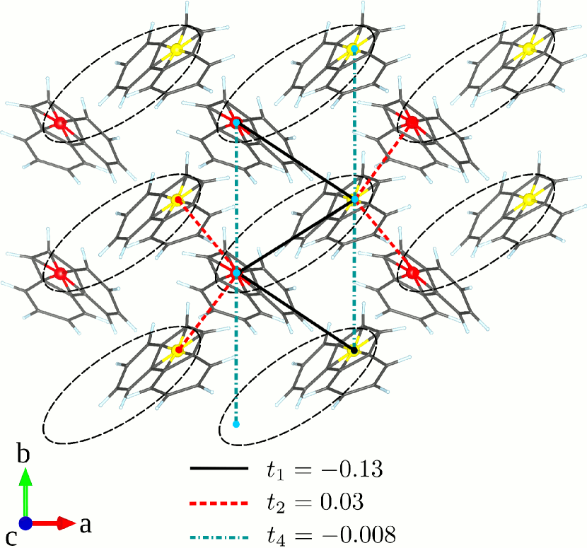
Figure 1: (Color online) Schematic molecular lattice model, adapted from Ref. Naghavi et al., 2013. Inter-molecular electron hopping matrix elements $t_{1}$, $t_{2}$, $t_{4}$ are marked. The inter-site dimerizing phonon between sites connected by the black line is responsible for the superconductivity in the Hubbard-Fröhlich model in Eq. (1).

We start off with the two-band tight-binding model recently proposed in Ref. Naghavi et al., 2013. The assumed three-dimensional lattice sketched in Fig.  1 has $\mathrm{P2_{1}}$ symmetry, typical of many even if not all pristine PAHs Naghavi et al. (2013); Casula et al. (2012); Kosugi et al. (2011b), with two equivalent sites per cell. An important symmetry element is the screw axis, which transforms one molecule onto the other, through a rotation accompanied by a fractional translation. Each site is endowed with a single nondegenerate orbital, representing the second lowest unoccupied molecular orbital (LUMO+1) of the neutral molecule. With an average of three electrons per molecule donated by electropositive atoms, (not included in the model), each molecular LUMO is completely filled and can be ignored, so that the LUMO+1 derived states that are precisely the half filled band that must be treated. Electrons in this orbital hop between sites with matrix elements indicated in Fig. 1, modeled for specificity after calculations performed for a representative hypothetical metallic phase of La-phenanthrene, giving rise to a half-filled LUMO+1 derived pair of bands Naghavi et al. (2013) shown in Fig.2. As seen in this figure the screw axis symmetry causes an important partial degeneracy on the Brillouin zone boundary – the two bands "sticking" together Heine (1960) – near the Fermi level. Two additional ingredients of the model are an intra-site Coulomb "Hubbard" $U$, and a "Fröhlich" coupling of electronic states to an inter-site phonon, whose key feature is a "dimerizing" character. A dimerizing displacement brings nearest molecules closer to form pairs, and is precisely such as to remove the screw axis, thus splitting the band degeneracy near Fermi level. Naghavi et al. (2013) We note here by analogy that the ability to split a band degeneracy near the Fermi level (that of the $\sigma$ bonding band top) is the basic reason why the famous $E_{g}$ phonon is so very effectively driving superconductivity in $\mathrm{MgB_{2}}$. Liu et al. (2001) The Hubbard-Fröhlich model Hamiltonian is

$$\mathcal{H}=\mathcal{H}_{0}+\mathcal{H}_{\mathrm{ph}}+\mathcal{H}_{\mathrm{el-ph}}+\mathcal{H}_{\mathrm{U}},$$ (1)

where electron hopping is

$$\mathcal{H}_{0}=\sum_{\mathbf{k}\sigma}\left(\begin{array}[]{cc}c_{1\mathbf{k}\sigma}^{\dagger}&c_{2\mathbf{k}\sigma}^{\dagger}\end{array}\right)\left(\begin{array}[]{cc}t_{\mathbf{k}}&t_{\mathbf{k}}^{12}\\ t_{\mathbf{k}}^{12\ast}&t_{\mathbf{k}}\end{array}\right)\left(\begin{array}[]{c}c_{1\mathbf{k}\sigma}^{\phantom{\dagger}}\\ c_{2\mathbf{k}\sigma}^{\phantom{\dagger}}\end{array}\right),$$ (2)

where $c^{\dagger}_{1(2)\mathbf{k}\sigma}$ creates a spin-$\sigma$ electron at momentum $\mathbf{k}$ in molecule 1(2). $\mathcal{H}_{0}$ in Eq. (2) gives rise to the half filled bands of Fig. 2. While we believe that many of the results to be derived later have a sufficient level of generality, the matrix elements in (2) are borrowed for specificity from an electronic structure calculation in Ref. Naghavi et al., 2013 and are

$$t_{\mathbf{k}} = 2\Big{(}t_{4}\,\cos k_{y}+t_{5}\,\cos k_{z}+t_{6}\,\cos\left(k_{x}+k_{z}\right)\Big{)},$$ (3)

$$t^{12}_{\mathbf{k}} = \Big{(}1+\text{e}^{-ik_{y}}\Big{)}\Big{(}t_{1}+t_{2}\,\text{e}^{-ik_{x}}+t_{3}\,\text{e}^{ik_{z}}\Big{)}$$ (4)

$$\equiv-\text{e}^{-i\theta_{\mathbf{k}}}\;\tau_{\mathbf{k}},$$

where $t_{1}\simeq-0.13$ eV, $t_{2}\simeq 0.03$ eV, $t_{3}\simeq 0.07$ eV, $t_{4}\simeq-0.008$ eV, $t_{5}\simeq 0.014$ eV, and finally $t_{6}\simeq 0.013$ eV.Naghavi et al. (2013) Recent calculations for K₃-phenanthrene, Naghavi and Tosatti (2014) a system where superconductivity has been observed Wang et al. (2011) lead to a LUMO+1 band structure that is similar, although different in the details.

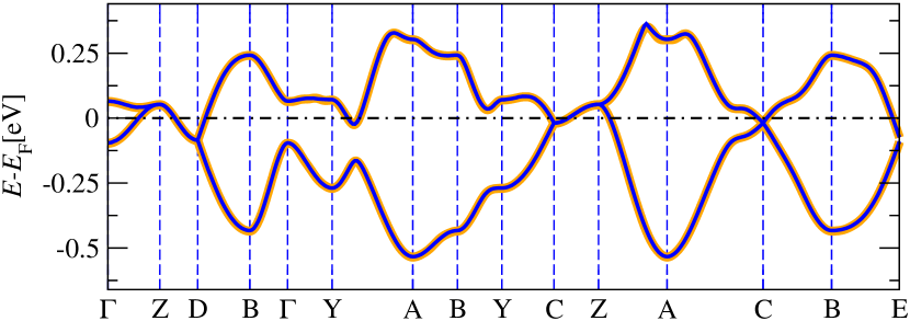
Figure 2: (Color online) The two half-filled bands used for the modeling, qualitatively representing LUMO+1 derived bands in a generic three-electron-doped polycyclic aromatic hydrocarbon. The specific form and parameters are from DFT results (black line) and their Wannier parametrization (orange line) obtained for hypothetical La-phenthrene in Ref. Naghavi et al., 2013.

As in Ref. Naghavi et al., 2013, and as indicated in Fig. 1, we only include in the model the inter-site phonon that modulates the hopping between molecule 1 and 2 along the $b$ direction, where the hybridization is stronger. This phonon has a dispersion

$$\mathcal{H}_{\mathrm{ph}}=\sum_{\mathbf{q}}\,\frac{\displaystyle\omega_{\mathbf{q}}}{\displaystyle 2}\;\Big{(}p_{\mathbf{q}}\,p_{-\mathbf{q}}+x_{\mathbf{q}}\,x_{-\mathbf{q}}\Big{)},$$ (5)

and is Fröhlich coupled to the conduction electrons via

$$\mathcal{H}_{\mathrm{el}-\mathrm{ph}}= \sum_{\mathbf{k},\mathbf{q},\sigma}x_{-\mathbf{q}}\,\left(\gamma_{\mathbf{k}+\mathbf{q}}+e^{i\mathbf{q}\cdot\mathbf{b}/2}\gamma_{\mathbf{k}}\right)\,c_{1\mathbf{k}\sigma}^{\dagger}c_{2\mathbf{k}+\mathbf{q}\sigma}^{\phantom{\dagger}}$$

$$+x_{-\mathbf{q}}\left(\gamma_{-\mathbf{k}}+e^{i\mathbf{q}\cdot\mathbf{b}/2}\gamma_{-\mathbf{k}-\mathbf{q}}\right)\,c_{2\mathbf{k}\sigma}^{\dagger}c_{1\mathbf{k}+\mathbf{q}\sigma}^{\phantom{\dagger}}.$$ (6)

Finally, the Hubbard repulsion is

$$\mathcal{H}_{\mathrm{U}}=U\,\sum_{\bm{R}}\,n_{1\bm{R}\uparrow}\,n_{1\bm{R}\downarrow}+n_{2\bm{R}\uparrow}\,n_{2\bm{R}\downarrow}.$$ (7)

At half-filling, the Hamiltonian (1) has in principle two competing instabilities: (i) antiferromagnetic insulator, the two molecules in the unit cell with opposite spin-$\frac{1}{2}$ polarization; (ii) phonon-mediated superconductivity. Antiferromagnetism is frustrated by the $k$-dependent diagonal elements in the hopping matrix of Eq. (2), and can be expected to prevail only above a threshold value of the repulsion $U$. The phonon-mediated Cooper instability only requires a finite density of states at the chemical potential and, since the pairing channel is intermolecular, it might be able to escape the intramolecule repulsion $U$. This qualitative reasoning leads us to expect that superconductivity might occur below a critical $U_{c}$, and antiferromagnetism above that. This simple-minded expectation will be explored and substantiated by calculations in the following sections.

III Mean field solution

The simplest tool to search for instabilities in an interacting electron model is the Hartree-Fock approximation. In our case, this is complicated by the retardation of the phonon-mediated electron-electron interaction. As in BCS theory, we shall neglect retardation and approximate the phonon-mediated interaction $\mathcal{H}_{\text{el-el}}$ by an instantaneous attraction that we will assume to act between electrons closer to the Fermi energy than a cutoff energy of order the Debye frequency.

The first mean-field step is diagonalizing the noninteracting Hamiltonian $\mathcal{H}_{0}$ in Eq. (2). This is done by applying the unitary transformation [see Eqs. (3) and (4)]

$$c_{g\mathbf{k}\sigma}^{\dagger} = \frac{\displaystyle 1}{\displaystyle\sqrt{2}}\;\Big{(}c_{1\mathbf{k}\sigma}^{\dagger}+\text{e}^{i\theta_{\mathbf{k}}}\;c_{2\mathbf{k}\sigma}^{\dagger}\Big{)},$$ (8)

$$c_{u\mathbf{k}\sigma}^{\dagger} = \frac{\displaystyle 1}{\displaystyle\sqrt{2}}\;\Big{(}c_{1\mathbf{k}\sigma}^{\dagger}-\text{e}^{i\theta_{\mathbf{k}}}\;c_{2\mathbf{k}\sigma}^{\dagger}\Big{)},$$ (9)

which leads to

$$\mathcal{H}_{0}=\sum_{\mathbf{k}\sigma}\,\xi_{g\mathbf{k}}\,c_{g\mathbf{k}\sigma}^{\dagger}\,c_{g\mathbf{k}\sigma}^{\phantom{\dagger}}+\xi_{u\mathbf{k}}\,c_{u\mathbf{k}\sigma}^{\dagger}\,c_{u\mathbf{k}\sigma}^{\phantom{\dagger}},$$ (10)

where $\xi_{g\mathbf{k}}=t_{\mathbf{k}}-\tau_{\mathbf{k}}-\mu$ and $\xi_{u\mathbf{k}}=t_{\mathbf{k}}+\tau_{\mathbf{k}}-\mu$ are the energies measured with respect to the chemical potential $\mu$.

Since superconductivity acts between time-reversed partners, pairing must be intra-band. We thus concentrate on the spin-singlet pair-creation operators

$$\Delta^{\dagger}_{g\mathbf{k}} = c^{\dagger}_{g\mathbf{k}\uparrow}c^{\dagger}_{g-\mathbf{k}\downarrow}+c^{\dagger}_{g-\mathbf{k}\uparrow}c^{\dagger}_{g\mathbf{k}\downarrow},$$ (11)

$$\Delta^{\dagger}_{u\mathbf{k}} = c^{\dagger}_{u\mathbf{k}\uparrow}c^{\dagger}_{u-\mathbf{k}\downarrow}+c^{\dagger}_{u-\mathbf{k}\uparrow}c^{\dagger}_{u\mathbf{k}\downarrow},$$ (12)

of each band, with energies $2\xi_{g\mathbf{k}}$ and $2\xi_{u\mathbf{k}}$, respectively. The Fröhlich-type of electron-phonon coupling, Eq. (6), can generate either an inter-molecular pairing (see Sec. (VI) for details.)

$$\propto\, \;-\big{(}c^{\dagger}_{1\mathbf{k}\uparrow}c^{\dagger}_{2-\mathbf{k}\downarrow}\,c^{\phantom{\dagger}}_{1-\mathbf{k^{\prime}}\downarrow}c^{\phantom{\dagger}}_{2\mathbf{k^{\prime}}\uparrow}+c^{\dagger}_{2\mathbf{k}\uparrow}c^{\dagger}_{1-\mathbf{k}\downarrow}\,c^{\phantom{\dagger}}_{2-\mathbf{k^{\prime}}\downarrow}c^{\phantom{\dagger}}_{1\mathbf{k^{\prime}}\uparrow}\big{)}$$

$$\sim-\big{(}\Delta^{\dagger}_{g\mathbf{k}}-\Delta^{\dagger}_{u\mathbf{k}}\big{)}\big{(}\Delta^{\phantom{\dagger}}_{g\mathbf{k^{\prime}}}-\Delta^{\phantom{\dagger}}_{u\mathbf{k^{\prime}}}\big{)},$$ (13)

or a pair hopping term

$$\propto\, \;-\big{(}c^{\dagger}_{1\mathbf{k}\uparrow}c^{\dagger}_{1-\mathbf{k}\downarrow}\,c^{\phantom{\dagger}}_{2-\mathbf{k^{\prime}}\downarrow}c^{\phantom{\dagger}}_{2\mathbf{k^{\prime}}\uparrow}+c^{\dagger}_{2\mathbf{k}\uparrow}c^{\dagger}_{2-\mathbf{k}\downarrow}\,c^{\phantom{\dagger}}_{1-\mathbf{k^{\prime}}\downarrow}c^{\phantom{\dagger}}_{1\mathbf{k^{\prime}}\uparrow}\big{)}$$

$$\sim-\big{(}\Delta^{\dagger}_{g\mathbf{k}}+\Delta^{\dagger}_{u\mathbf{k}}\big{)}\big{(}\Delta^{\phantom{\dagger}}_{g\mathbf{k^{\prime}}}+\Delta^{\phantom{\dagger}}_{u\mathbf{k^{\prime}}}\big{)},$$ (14)

which, when combined, justify the following expression for the phonon-mediated attraction that we shall consider hereafter:

$$\mathcal{H}_{\mathrm{ep-eff}}=-\frac{\displaystyle g_{\ast}}{\displaystyle 2V}\sum_{\mathbf{k}\mathbf{k^{\prime}}}\,s_{\mathbf{k}}\,s_{\mathbf{k^{\prime}}}\Big{(}\Delta_{g\mathbf{k}}^{\dagger}\,\Delta_{g\mathbf{k^{\prime}}}^{\phantom{\dagger}}+\Delta_{u\mathbf{k}}^{\dagger}\,\Delta_{u\mathbf{k^{\prime}}}^{\phantom{\dagger}}\Big{)}.$$ (15)

Here $g_{\ast}$ is the effective attractive potential, which is of the order of the square of the typical electron-phonon coupling constant $\gamma$, see Eq. (6), divided by the typical phonon frequency. As mentioned, we neglect retardation but introduce a function $s_{\mathbf{k}}$ which is +1 if $\left|\xi_{g(u)\mathbf{k}}\right|\leq\hbar\omega_{D}$ with $\omega_{D}$ the typical phonon frequency, and zero otherwise.

The Hubbard repulsion, once projected onto the intra-band singlet Cooper channels, reads as

$$\mathcal{H}_{\mathrm{U}}=\frac{U}{8V}\sum_{\mathbf{k}\mathbf{k^{\prime}}}\left(\Delta_{g\mathbf{k}}^{\dagger}+\Delta_{u\mathbf{k}}^{\dagger}\right)\left(\Delta_{g\mathbf{k^{\prime}}}+\Delta_{u\mathbf{k^{\prime}}}\right).$$ (16)

We solve the Hamiltonian $\mathcal{H}=\mathcal{H}_{0}+\mathcal{H}_{\mathrm{ep-eff}}+\mathcal{H}_{\mathrm{U}}$ within the Hartree-Fock approximation (HF). Assuming the two order parameters

$$\bar{\Delta}_{g\mathbf{k}}^{\ast} = \left\langle\Delta_{g\mathbf{k}}^{\dagger}\right\rangle,$$ (17)

$$\bar{\Delta}_{u\mathbf{k}}^{\ast} = \left\langle\Delta_{u\mathbf{k}}^{\dagger}\right\rangle,$$ (18)

the gap equations are

$$\bar{\Delta}_{g\left(u\right)\mathbf{k}}=\frac{\displaystyle D_{g\left(u\right)\mathbf{k}}}{\displaystyle E_{g\left(u\right)\mathbf{k}}}\;\bigg{[}2f\big{(}E_{g\left(u\right)\mathbf{k}}\big{)}-1\bigg{]},$$ (19)

where $f(E)$ is the Fermi-Dirac distribution at temperature $T$, and

$$D_{g\left(u\right)\mathbf{k}} = \frac{1}{V}\sum_{\mathbf{k^{\prime}}}\Bigg{[}\frac{U}{4}\,\Big{(}\bar{\Delta}_{g\left(u\right)\mathbf{k^{\prime}}}+\bar{\Delta}_{u\left(g\right)\mathbf{k^{\prime}}}\Big{)}$$ (20)

$$\qquad\qquad-g_{\ast}\,s_{\mathbf{k}}\,s_{\mathbf{k^{\prime}}}\;\bar{\Delta}_{g\left(u\right)\mathbf{k^{\prime}}}\Bigg{]},$$

$$E_{g\left(u\right)\mathbf{k}} = \sqrt{\xi_{g\left(u\right)\mathbf{k}}^{2}+D_{g\left(u\right)\mathbf{k}}^{2}}\,,$$ (21)

with the additional assumption that $\bar{\Delta}_{g\left(u\right)\mathbf{k}}$ is real. We also need to fix the chemical potential $\mu$ so that the density corresponds to one electron per site, which brings about another self-consistency equation besides (19).

Before discussing the solution of the self-consistency equations, it is worth remarking that, if $U>4g_{\ast}$, as is expected to be the case, the whole interaction, Eq. (16) plus Eq. (15), is repulsive everywhere in momentum space, although its value jumps from $U-4g_{\ast}$ when $s_{\mathbf{k}}\,s_{\mathbf{k^{\prime}}}=1$ up to $U$ when $s_{\mathbf{k}}\,s_{\mathbf{k^{\prime}}}=0$. In spite of that overall repulsion, superconductivity can still as we shall see be stabilized by two conspiring facts: (1) the high-energy screening of the Hubbard $U$ which results into an effectively lower repulsion, which in the long-range case results in the so-called Coulomb pseudo-potential felt by the electrons close to Fermi level;Morel and Anderson (1962) (2) the opposite sign which can be chosen by the two order parameters $\bar{\Delta}_{g\mathbf{k}}$ and $\bar{\Delta}_{u\mathbf{k}}$ radically reducing the strength of the Hubbard repulsion, see Eq. (16), an $s_{\pm}$-wave symmetry similar to the Suhl-Kondo scheme for band-overlapping superconductors.Suhl et al. (1959); Kondo (1963) In fact, we note that, among the two pairing channels Eqs. (13) and (14) that can be stabilized by the electron-phonon coupling Eq. (6), only the former, which corresponds to an inter-molecule spin-singlet pairing, is not hindered by the Hubbard repulsion Eq. (16), thus naturally explaining the reason of the sign difference between $\bar{\Delta}_{g\mathbf{k}}$ and $\bar{\Delta}_{u\mathbf{k}}$. In other words, it is crucial for the stabilization of superconductivity despite the Hubbard repulsion that electrons couple to phonons in a Fröhlich’s inter-site rather than Holstein’s intra-site fashion, i.e. by a phonon-modulated hopping rather than by a phonon-induced charge attraction.

III.1 Hartree Fock Results

We solved numerically the Hartree-Fock self-consistency equations, Eq. (19) with the condition that fixes the chemical potential, using the tight-binding parameters extracted in Ref. Naghavi et al., 2013, and reasonable estimates of the electron-phonon coupling $g_{\ast}=100$ meV and of the cut-off Debye frequency $\hbar\omega_{D}=10$ meV.Subedi and Boeri (2011); Casula et al. (2011, 2012); Girlando et al. (2012) As a parameter, we considered a variable electron repulsion $U$ below 1.0 eV,Nomura et al. (2012) still reaching and even surpassing the bandwidth, so as to assess its importance in connection with superconductivity. As anticipated, see Fig. 3, the two gaps acquire opposite sign $\bar{\Delta}_{g\bm{k}}\bar{\Delta}_{u\bm{k}}<0$ in the main symmetry directions, so that the cancellation between $\bar{\Delta}_{g\bm{k}}$ and $\bar{\Delta}_{u\bm{k}}$ preserves superconductivity in spite of a substantial repulsion. In addition, both gaps change sign at an energy equal to the cutoff $\hbar\omega_{D}$; the standard manifestation of the the high-energy screening. Morel and Anderson (1962) As a result, the gap values (Fig. 4) are remarkably insensitive to the growth of $U$ in a broad range. In Figs. 4 and 5 the even and odd superconducting gaps $\tilde{\Delta}_{g}$ and $\tilde{\Delta}_{u}$ are defined as averages over the Fermi surfaces.

In Fig. 5, we show instead the gaps $\tilde{\Delta}_{g}$ and $\tilde{\Delta}_{u}$ as function of temperature. With the assumed parameters we can estimate $T_{c}\sim 3$ K, in fact not dissimilar to the experimental ones.Wang et al. (2012) We should probably regard that order of magnitude agreement as coincidental, both the model and the approximations being rather generic.

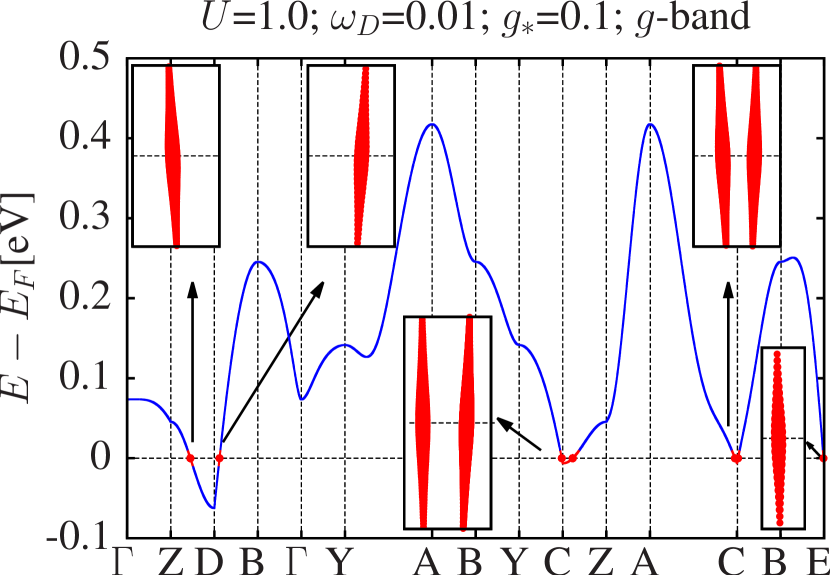
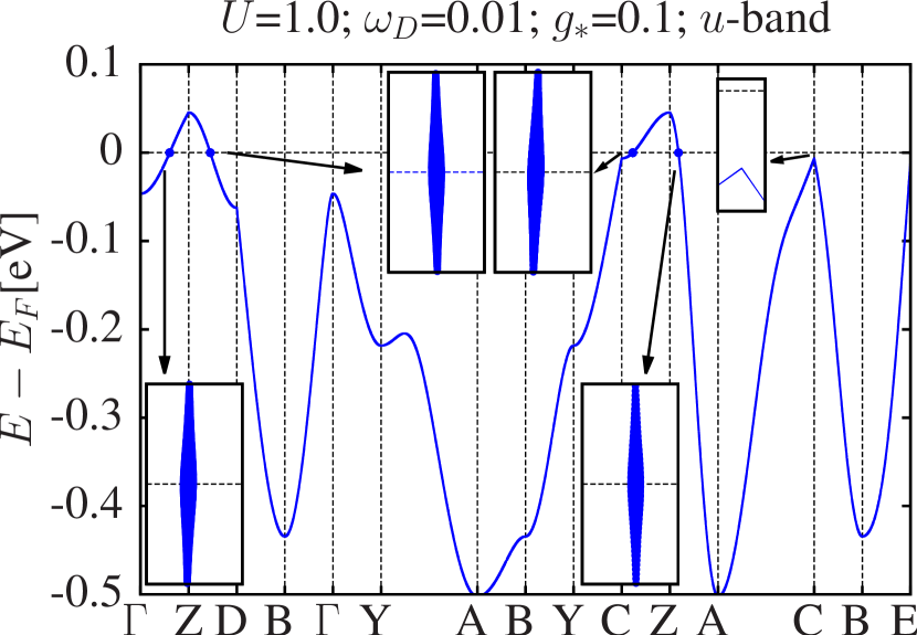
Figure 3: (Color online) Energy bands and gap parameters in the main symmetry directions in the $\bm{k}$ space at zero temperature. The insets show the magnified gap parameters near the Fermi level: width proportional to amplitude, blue and red colors indicates positive and negative sign.

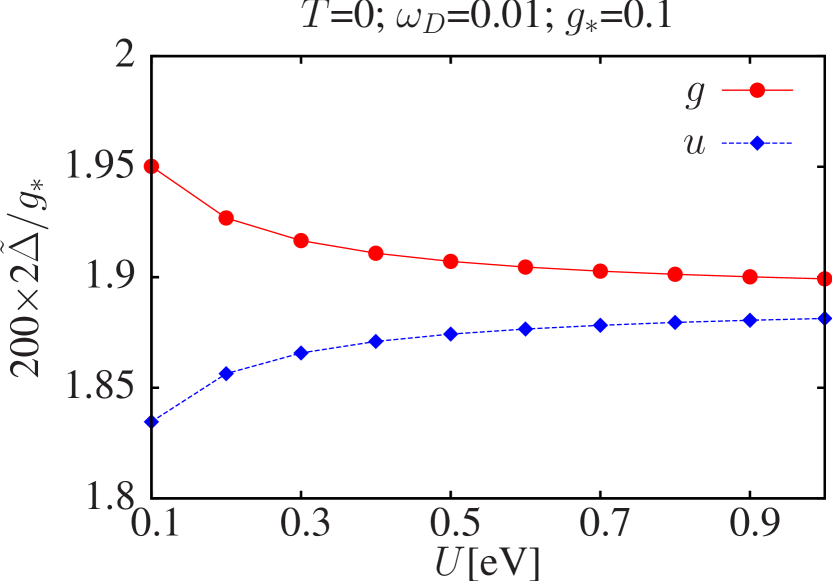
Figure 4: (Color online) $T$=0 mean-field energy gap magnitudes are robust for increasing Hubbard $U$.

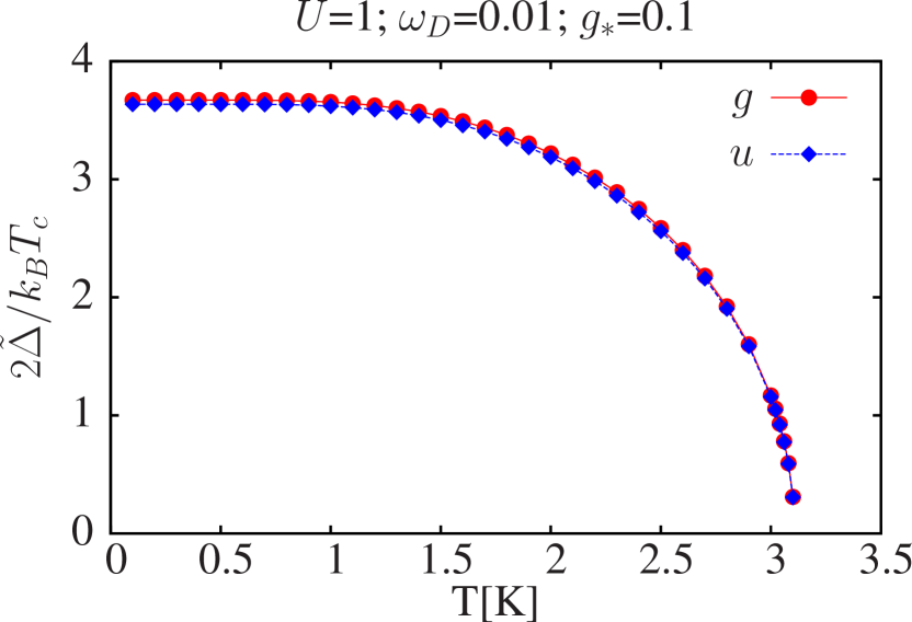
Figure 5: (Color online) Mean-field temperature dependence of energy gaps. Parameters such as those of Ref. Naghavi et al., 2013 would lead to an estimated $T_{c}\sim$ 3 K.

IV Gutzwiller Correlations and Gutzwiller Approximation

In the previous section, we found that a variational BCS state can be stabilized within the Hartree-Fock approximation in spite of a relatively strong Coulomb repulsion, thanks to an order parameter that develops opposite sign in the two bands, an $s_{\pm}$-wave symmetrySuhl et al. (1959); Kondo (1963). This sign change suppresses the onsite amplitude of the pair wave function, thus reducing the energy cost of the Hubbard $U$. As we already mentioned [see Eq. (13)], the property $\bar{\Delta}_{g\bm{k}}\,\bar{\Delta}_{u\bm{k}}<0$ is in reality a characteristic of an inter-site pairing

$$c^{\dagger}_{1\mathbf{k}\uparrow}c^{\dagger}_{2-\mathbf{k}\downarrow}+c^{\dagger}_{2-\mathbf{k}\uparrow}c^{\dagger}_{1\mathbf{k}\downarrow}\sim\Delta_{g\mathbf{k}}^{\dagger}-\Delta_{u\mathbf{k}}^{\dagger},$$ (22)

as opposed to an on-site one. In other words, the sign difference is brought here by the pairing mechanism itself rather than by the competition with onsite repulsion. As a matter of fact, the latter may actually strengthen pairing. In fact, as $U$ increases, the time each pair of neighboring molecules spend in the configuration where both are singly occupied increases, leaving enough time for the molecules to couple into an inter-site spin-singlet thus gaining electron-phonon energy before the electrons escape.

The Hartree-Fock approximation is not fully able to grasp this repulsion-reinforced pairing, exhibiting a superconducting gap that does not grow but rather saturates for large $U$ (see Fig. 4). This limitation of the Hartree-Fock approximation does not come as a surprise, since the method is not reliable when the interaction is comparable or even larger than the bandwidth. This uncertainty becomes crucial if we must compare the superconducting state energy with other possible ground states that on the contrary take advantage of a greater $U$, most notably an antiferromagnetic insulator with molecule 1 spin-polarized opposite to molecule 2. Physically, large $U$ tends to Mott localize the charge by suppressing configurations where two electrons occupy the same LUMO+1 molecular orbital. In order not to waste too much kinetic and ionic-potential energy, the electrons must coordinate among each other so to avoid sharing the same molecule during their motion. This electron self-organization occurs at large $U$ in correspondence with charge localization. Antiferromagnetism is but a strategy to synchronize electron motion, forcing nearby molecules to be occupied by opposite spin electrons which can therefore exchange. Antiferromagnetism has indeed been shown to arise as the lowest-energy solution within density functional theory calculations of alkali-doped aromatics Giovannetti and Capone (2011). Our point here is that the true system has other strategies at its disposal. In fact, efficient correlations avoiding double occupancy can also develop within an overall singlet and metallic ground state, including the above $s_{\pm}$ superconducting state stabilized by the Fröhlich’s electron-phonon coupling. In order to explore that possibility and establish the most efficient correlation strategy, one needs a better approach than mean-field ones. The improved approximation should be able, unlike mean field, to disentangle charge, whose fluctuations are suppressed by a large $U$, from spin and orbital degrees of freedom which are not. For that purpose, we used a variational search within the class of Gutzwiller-type wave functions Gutzwiller (1964, 1965), much broader than Hartree-Fock which includes just Slater determinants and BCS wavefunctions. In addition, we also adopted the so-called Gutzwiller approximation (GA) to evaluate the average values of any operator on the Gutzwiller wave function, an approximation that becomes exact in the limit of lattices with infinite coordination Bünemann et al. (1998); Fabrizio (2007, 2013).

IV.1 Gutzwiller method

The Gutzwiller variational wave function we shall consider is defined through

$$\left|\Psi_{G}\right\rangle=\prod_{\bm{R}}\prod_{a=1,2}\,\mathcal{P}_{a\bm{R}}\,\left|\Psi_{0}\right\rangle,$$ (23)

where $\mathcal{P}_{a\bm{R}}$ is a linear operator that depends on a set of variational parameters and acts on the LUMO+1 Hilbert space of molecule $a=1,2$ in the unit cell $\mathbf{R}$, while $\left|\Psi_{0}\right\rangle$ is a variational Slater determinant or BCS wave function. $P_{a\bm{R}}$ therefore provides the new variational freedom with respect to Hartree-Fock. We impose the following pair of constraints Bünemann et al. (1998); Fabrizio (2007, 2013):

$$\left\langle\Psi_{0}\right|\mathcal{P}_{a\bm{R}}^{\dagger}\,\mathcal{P}_{a\bm{R}}^{\phantom{\dagger}}\left|\Psi_{0}\right\rangle= 1,$$ (24)

$$\left\langle\Psi_{0}\right|\mathcal{P}_{a\bm{R}}^{\dagger}\,\mathcal{P}_{a\bm{R}}^{\phantom{\dagger}}\,n_{a\bm{R}\sigma}\left|\Psi_{0}\right\rangle= \left\langle\Psi_{0}\right|n_{a\bm{R}\sigma}\left|\Psi_{0}\right\rangle,$$ (25)

where $n_{a\mathbf{R}\sigma}$ is the number operator of spin-$\sigma$ electrons on the LUMO+1 of molecule $a$ at site $\mathbf{R}$. Within the GA, and upon enforcing the above constraints, the following expressions are assumed, which are exact in infinite-coordination lattices,

$$\left\langle\Psi_{G}\right|\hat{O}_{a\bm{R}}\left|\Psi_{G}\right\rangle = \left\langle\Psi_{0}\right|\,\mathcal{P}_{a\bm{R}}^{\dagger}\,\hat{O}_{a\bm{R}}\,\mathcal{P}_{a\bm{R}}^{\phantom{\dagger}}\left|\Psi_{0}\right\rangle,$$

$$\left\langle\Psi_{G}\right|\hat{O}_{a\bm{R}}\,\hat{O}_{b\bm{R}^{\prime}}\left|\Psi_{G}\right\rangle = \left\langle\Psi_{0}\right|\mathcal{P}_{a\bm{R}}^{\dagger}\,\hat{O}_{a\bm{R}}\,\mathcal{P}_{a\bm{R}}^{\phantom{\dagger}}$$

$$\qquad\qquad\mathcal{P}_{b\bm{R}^{\prime}}^{\dagger}\,\hat{O}_{b\bm{R}^{\prime}}\,\mathcal{P}_{b\bm{R}^{\prime}}^{\phantom{\dagger}}\left|\Psi_{0}\right\rangle,$$

where $\hat{O}_{a\bm{R}}$ is any local operator. The right hand sides of both equations can be simply evaluated using Wick’s theorem, which holds both for Slater determinants and BCS wave functions.

The Hamiltonian we shall employ from now on is a further simplification of the original one in Sec. II. We already noticed that, among the two pairing channels, Eqs. (13) and (14), only the first is able to circumvent a strong on-site repulsion. Therefore, we dismiss the pair hopping (14) and approximate the phonon-mediated electron-electron interaction by the inter-site pairing (13), which we rewrite as

$$\mathcal{H}_{\text{ep-eff}}\rightarrow\mathcal{H}_{\text{J}} = J\,\sum_{\mathbf{R}}\,\mathbf{S}_{1\mathbf{R}}\cdot\mathbf{S}_{2\mathbf{R}}$$ (26)

$$+J\,\sum_{\mathbf{R}}\,\mathbf{S}_{1\mathbf{R}}\cdot\mathbf{S}_{2\mathbf{R}+\mathbf{b}},$$

where $\mathbf{S}_{a\mathbf{R}}$ is the spin-operator of molecule $a=1,2$ at site $\mathbf{R}$ and the second sum is restricted to nearest-neighbor molecules on different cells along the $\mathbf{b}$ direction. Here, $J$ has the same magnitude of $g_{*}$ in Eq. (15), and, for the sake of simplicity, we ignore the retardation effects brought in by the functions $s_{\mathbf{k}}$ in (15). This actually implies an underestimate of superconductivity, by not allowing for high-energy screening. Equation (26) also omits additional charge attraction between the molecules, which does not play any relevant role for large $U$Plekhanov et al. (2003). The total simplified Hamiltonian then reads as

$$\mathcal{H}=\mathcal{H}_{0}+\mathcal{H}_{\mathrm{U}}+\mathcal{H}_{\mathrm{J}},$$ (27)

and is a two-band version of the so-called $t$-$J$-$U$ model sometimes used in the context of high-$T_{c}$ superconductorsZhang (2003); Plekhanov et al. (2003), even though $J$ is provided here by electron-phonon coupling and not by projecting a purely electronic Hamiltonian onto low-energy Zhang-Rice singlets of doped CuO₂ planesZhang and Rice (1988).

We shall consider two possible variational wave-functions: a superconducting (SC) and an antiferromagnetic (AF) one. In the AF state, molecule 1 is $\uparrow$ spin-polarized and molecule 2 is $\downarrow$ spin-polarized and the corresponding "uncorrelated" wave function $|\Psi_{0}\rangle$ is characterized by

$$\langle\Psi_{0}|\,n_{1\,\mathbf{R}\uparrow}-n_{1\,\mathbf{R}\downarrow}\,|\Psi_{0}\rangle = -\langle\Psi_{0}|\,n_{2\,\mathbf{R}\uparrow}-n_{2\,\mathbf{R}\downarrow}\,|\Psi_{0}\rangle$$ (28)

$$=2m,\qquad\forall\mathbf{R}.$$

By contrast, the SC state has a spin-singlet intermolecular pairing as in Eq. (22), which we assume real, and its uncorrelated wave function is thus characterized by

$$\langle\Psi_{0}|\,c^{\dagger}_{1\mathbf{R}\uparrow}c^{\dagger}_{2\mathbf{R^{\prime}}\downarrow}+c^{\dagger}_{2\mathbf{R^{\prime}}\uparrow}c^{\dagger}_{1\mathbf{R}\downarrow}\,|\Psi_{0}\rangle=\Delta^{(0)}_{\mathbf{R}\mathbf{R^{\prime}}}.$$ (29)

In both SC and AF cases, the linear operator $\mathcal{P}_{a\mathbf{R}}$ can be generally written as

$$\mathcal{P}_{a\mathbf{R}} = \lambda_{0}\,|0_{a\mathbf{R}}\rangle\langle 0_{a\mathbf{R}}|+\lambda_{2}\,|2_{a\mathbf{R}}\rangle\langle 2_{a\mathbf{R}}|$$ (30)

$$+\lambda_{a\,\uparrow}\,|\uparrow_{a\mathbf{R}}\rangle\langle\uparrow_{a\mathbf{R}}|+\lambda_{a\,\downarrow}\,|\downarrow_{a\mathbf{R}}\rangle\langle\downarrow_{a\mathbf{R}}|,$$

in terms of projectors onto states with well-defined occupancies and spin of the LUMO+1 orbital of molecule $a$ at site $\mathbf{R}$, 0 standing for empty, 2 for doubly occupied, and $\uparrow(\downarrow)$ for singly occupied with $\uparrow(\downarrow)$ spin. The variational parameters collectively designated as $\lambda$, which we can restrict to be real in this specific case, do not depend on the unit cell $\mathbf{R}$ because we assume full translational symmetry. In addition, we shall not consider any charge disproportionation between the two molecules, then $\lambda_{0}$ and $\lambda_{2}$ are independent of $a$. On the contrary, in the AF case we must allow for $\lambda_{1\,\uparrow}=\lambda_{2\,\downarrow}\not=\lambda_{1\,\downarrow}=\lambda_{2\,\uparrow}$ consistently with the antiferromagnetic ordering, while the spin-singlet SC obviously implies $\lambda_{1\,\uparrow}=\lambda_{2\,\downarrow}=\lambda_{1\,\downarrow}=\lambda_{2\,\uparrow}$.

We introduce the uncorrelated probability distribution $P^{(0)}_{a\alpha}=\langle\Psi_{0}|\,|\alpha_{a\mathbf{R}}\rangle\langle\alpha_{a\mathbf{R}}|\,|\Psi_{0}\rangle$, which is independent of $\mathbf{R}$ and where $\alpha=0,2,\uparrow,\downarrow$, and the correlated one $P_{a\alpha}=\langle\Psi_{G}|\,|\alpha_{a\mathbf{R}}\rangle\langle\alpha_{a\mathbf{R}}|\,|\Psi_{G}\rangle$, which is readily found to be

$$P_{a\,0} = \left|\lambda_{0}\right|^{2}\,P^{(0)}_{a\,0}=\frac{1}{4}\;\left|\lambda_{0}\right|^{2}\equiv P_{0},$$

$$P_{a\,2} = \left|\lambda_{2}\right|^{2}\,P^{(0)}_{a\,2}=\frac{1}{4}\;\left|\lambda_{2}\right|^{2}\equiv P_{2},$$

$$P_{1\,\uparrow} = \left|\lambda_{1\,\uparrow}\right|^{2}\,P^{(0)}_{1\,\uparrow}=\left|\lambda_{1\,\uparrow}\right|^{2}\,\Big{(}\frac{1}{2}+m\Big{)}^{2}$$

$$= P_{2\,\downarrow}\equiv P_{\uparrow},$$

$$P_{1\,\downarrow} = \left|\lambda_{1\,\downarrow}\right|^{2}\,P^{(0)}_{1\,\downarrow}=\left|\lambda_{1\,\downarrow}\right|^{2}\,\Big{(}\frac{1}{2}-m\Big{)}^{2}$$

$$= P_{2\,\uparrow}\equiv P_{\downarrow},$$

valid for both AF ($m\not=0$) and SC ($m=0$).

Using these definitions, the constraints (24) and (25) for our assumed density corresponding to one electron per site (three electrons per molecule, but only one in the LUMO+1 orbital) take the simple form

$$P_{0}+P_{\uparrow}+P_{\downarrow}+P_{2} = 1,$$ (31)

$$P_{0} = P_{2},$$ (32)

$$P_{\uparrow}-P_{\downarrow} = 2m,$$ (33)

where in the SC wave function $P_{\uparrow}=P_{\downarrow}$ since $m=0$.

The average energy of the variational wave function and within the GA isFabrizio (2007)

$$E = R^{2}\,\langle\Psi_{0}|\,\mathcal{H}_{0}\,|\Psi_{0}\rangle$$ (34)

$$+\langle\Psi_{0}|\,\mathcal{H}_{*\,\text{J}}\,|\Psi_{0}\rangle+2\,N\,P_{0}\,U,$$

where $N$ is the number of unit cells,

$$R^{2}=\frac{\displaystyle 4P_{2}}{\displaystyle 1-4m^{2}}\;\Big{(}\sqrt{P_{\uparrow}}+\sqrt{P_{\downarrow}}\Big{)}^{2},$$ (35)

is a factor that renormalizes downwards the intersite hopping, (a factor whose square can be associated with the quasi-particle wave-function renormalization commonly denoted as $Z$), and $\mathcal{H}_{*\,\text{J}}$ has the same form of $\mathcal{H}_{\text{J}}$ provided the spin operators are modified according to $\mathbf{S}_{a\mathbf{R}}\rightarrow\mathcal{P}_{a\mathbf{R}}\,\mathbf{S}_{a\mathbf{R}}\,\mathcal{P}_{a\mathbf{R}}$, which implies that (we omit for convenience the unit cell index $\mathbf{R}$):

$$\mathcal{P}_{a}\,S^{z}_{a}\,\mathcal{P}_{a}\, = \frac{\displaystyle\lambda_{a\,\uparrow}^{2}+\lambda_{a\,\downarrow}^{2}}{\displaystyle 2}\;S^{z}_{a}$$

$$+\frac{\displaystyle\lambda_{a\,\uparrow}^{2}-\lambda_{a\,\downarrow}^{2}}{\displaystyle 2}\;\Big{(}n_{a\uparrow}+n_{a\downarrow}-2n_{a\uparrow}n_{a\downarrow}\Big{)},$$

$$\mathcal{P}_{a}\,S^{+}_{a}\,\mathcal{P}_{a}\, = \lambda_{a\,\uparrow}\,\lambda_{a\,\downarrow}\,S^{+}_{a}.$$

In the SC case one finds simply that $\mathcal{H}_{*\,\text{J}}=(4\,P_{\uparrow})^{2}\,\mathcal{H}_{\text{J}}=(4\,P_{\downarrow})^{2}\,\mathcal{H}_{\text{J}}$, showing that $J$ is renormalized to an effective $J_{*}=(4\,P_{\uparrow})^{2}\,J$, while in the AF case the expression becomes more involved.

The variational energy in Eq. (34) depends on the $\lambda$ parameters, subject to the constraints of Eqs. (31), (32), and(33). It also depends on the uncorrelated wave function $|\Psi_{0}\rangle$, which is in turn constrained to the $\lambda$ only in the AF case through Eq. (28). Here, we find it more convenient to treat $m$ as an additional variational parameter, imposing Eq. (28) via a Lagrange multiplier and (33) by simply setting $P_{\uparrow}=2m+P_{\downarrow}$ with $2P_{\downarrow}=1-2P_{0}-2m\geq 0$, and minimizing first with respect to $|\Psi_{0}\rangle$ and $P_{0}$ and finally to $m$. We observe that optimization with respect to $|\Psi_{0}\rangle$ amounts to find either the antiferromagnetic Slater determinant, subject to the constraint (28), or the BCS wave function, both of which minimize the average value of $\mathcal{H}_{*}=\mathcal{H}_{0}+\mathcal{H}_{*\,\text{J}}$. This is practically the same task as solving a Hartree-Fock problem. The following step, i.e., minimization with respect to $P_{0}$ and, in the AF case, to $m$, is similarly simple to accomplish, so that the full numerical optimization does not require a much greater effort than simple Hartree-Fock.

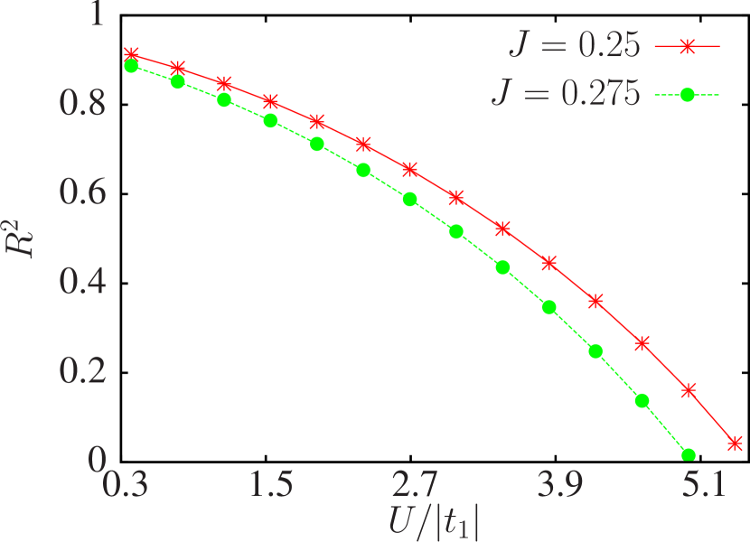
Figure 6: (Color online) Quasi-particle wave function renormalization factor $R^{2}$ of the superconducting state as function of $U$ in units of $|t_{1}|$. Note that $R^{2}$ goes continuously to 0, signaling a second-order Mott transition.

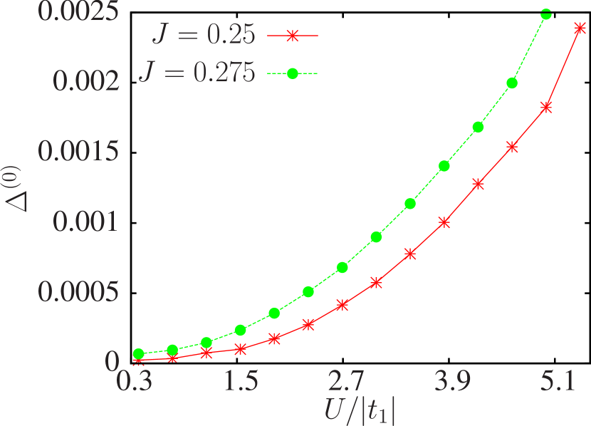
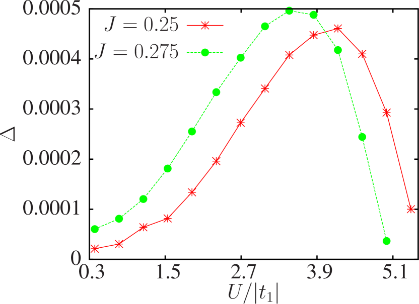
Figure 7: (Color online) Top panel: uncorrelated SC parameter $\Delta^{(0)}$ as function of $U$. Lower panel: true SC order parameter $\Delta$ as function of $U$.

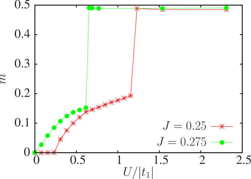
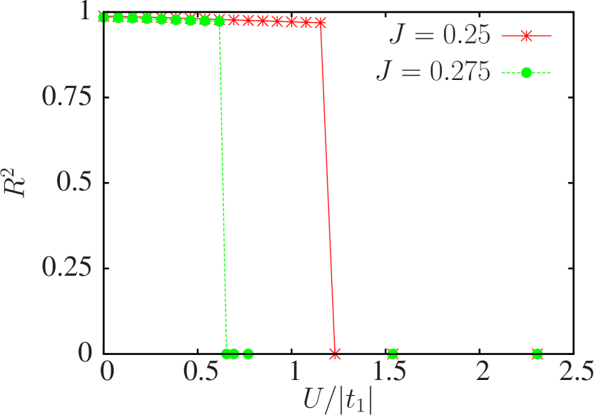
Figure 8: (Color online) Sublattice magnetization magnitude $m$ and renormalization factor $R^{2}$ of the antiferromagnetic state with $U/|t_{1}|$. With increasing $U$, $m\rightarrow\frac{1}{2}$ and the system reaches the atomic limit. The metal-Mott insulator transition is of first order.

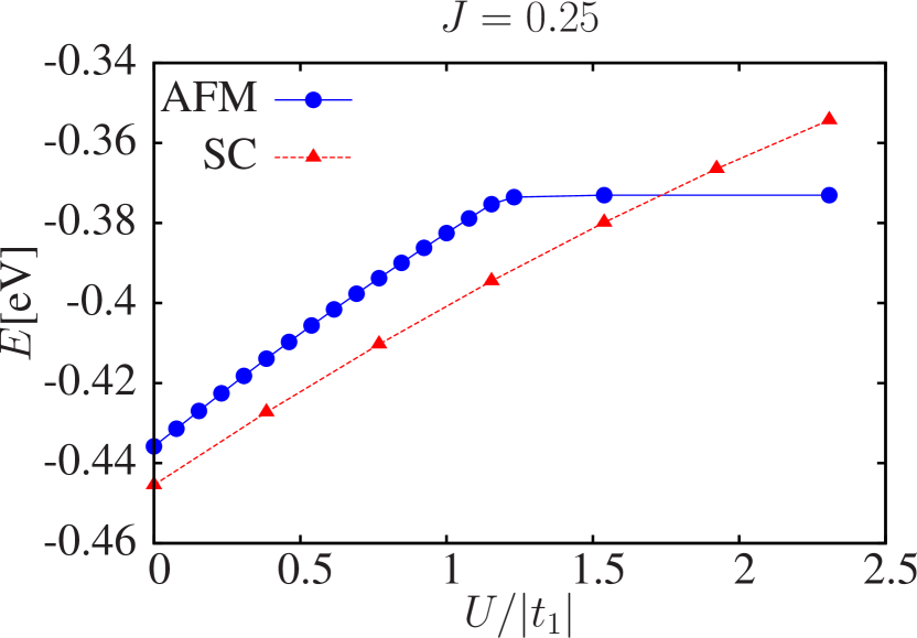
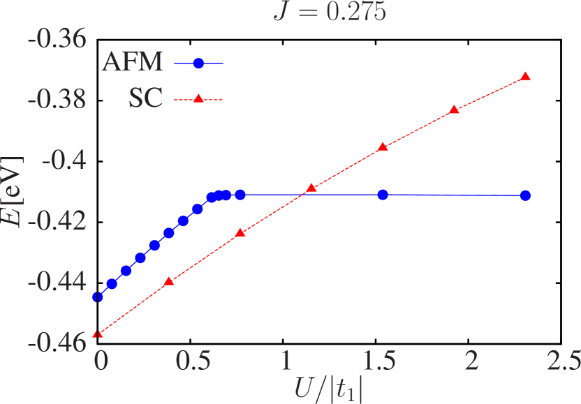
Figure 9: (Color online) Competition between ground-state energies of superconducting and antiferromagnetic states. Unlike mean field, where antiferromagnetism always prevails, superconductivity survives with Gutzwiller correlations where there is a SC-AF transition at $U/|t_{1}|\simeq 1.8$ for $J=0.25$, and $U/|t_{1}|\simeq 1.1$ for $J=0.275$.

IV.2 Results and discussion

We are now ready to present and discuss the results of the Gutzwiller variational approach for both SC and AF wave functions, starting from the former. We first note that the SC order parameter of the uncorrelated wave function, defined in Eq. (29) no longer coincides with the actual order parameter evaluated on $|\Psi_{G}\rangle$. In fact,

$$\Delta_{\mathbf{R}\mathbf{R^{\prime}}} \equiv \langle\Psi_{G}|\,c^{\dagger}_{1\mathbf{R}\uparrow}c^{\dagger}_{2\mathbf{R^{\prime}}\downarrow}+c^{\dagger}_{2\mathbf{R^{\prime}}\uparrow}c^{\dagger}_{1\mathbf{R}\downarrow}\,|\Psi_{G}\rangle$$ (36)

$$=R^{2}\,\Delta^{(0)}_{\mathbf{R}\mathbf{R^{\prime}}},$$

where the last expression derives from the GA. Since large $U$ suppresses double occupancy, that is $P_{2}=P_{0}\ll 1$, the renormalization factor $R\ll 1$. It is therefore possible to find an uncorrelated wave function $|\Psi_{0}\rangle$ with a large bare SC order parameter yet with just a tiny true order parameter after projection. As we shall see, this is the key feature of the Gutzwiller wave function that allows the stabilization of superconductivity despite a strong repulsion, in fact even in the vicinity of a Mott transition, and has been repeatedly invoked in the context of $t$-$J$ models for cupratesAnderson (1987); Paramekanti et al. (2001); Sorella et al. (2002).

In Fig. 6 we plot the wave-function renormalization factor $R^{2}$ as function of $U$. As expected, $R^{2}$ decreases monotonically with increasing $U$ and vanishes at a critical value that identifies the Mott transition. On the other hand, the inter-molecule SC order parameter $\Delta_{0}$ of the uncorrelated wave function increases with increasing $U$ (see top panel in Fig. 7). The joint result of these two variations is a non-monotonic variation of the true SC order parameter $\Delta$ [Eq. (36)], which first increases with $U$, reaches a maximum, and then drops and vanishes at the Mott transition ( see lower panel in the same Fig. 7). This detailed behavior contrasts with the insensitivity of the Hartree-Fock mean-field solution of previous sections (see Fig. 4).

That at first sight surprising behavior is actually explained by a physics not dissimilar to that invoked Refs. Capone et al., 2002 and Capone et al., 2009 to explain the robustness of intra-molecular $s$-wave superconductivity in alkali-doped fullerenes in spite of the strong Coulomb repulsion. As $U$ increases, the effective quasi-particle bandwidth is renormalized down by the factor $R^{2}<1$. At the same time, the effective strength of the attraction $J_{*}=(4\,P_{\uparrow})^{2}\,J$ does not drop. In the present case of Fröhlich intersite phonon pairing interaction $J_{*}$ actually increases, since the probability of single occupancy $P_{\uparrow}=P_{\downarrow}$ rises. The net result is that the system is pushed towards a strong coupling regime with an effective attraction of the same order of magnitude as the quasi-particle bandwidth. The reason why superconductivity is not damaged but is fostered instead by an increasing repulsion, is that, similarly to fulleride models, pairing in this model occurs in a channel orthogonal to chargeCapone et al. (2002, 2009).

We emphasize that these results are qualitatively not at all new, especially in the context $t$-$J$ models for cuprates. Indeed, exact calculations of Gutzwiller-projected wave functions, i.e., $P_{2}$ strictly zero but away from half-filling, using variational Monte Carlo already highlighted an increase of the uncorrelated order parameter upon approaching the undoped Mott insulator, as opposed to a reduction of the actual SC order parameterParamekanti et al. (2001); Sorella et al. (2002). However, these studies and calculations, which involved no phonons, dealt with $U\to\infty$, where metallic behavior is possible only at finite doping, whereas the half-filled system is trivially an antiferromagnetic Mott insulator. In our half-filled case, a correlated metallic and superconducting state is stable at small $U$, although it should eventually turn into an antiferromagnetic insulator above a critical $U_{c}$, which we must identify. For that purpose, we implement the GA for the AF state, which is the natural competitor of SC.

In Fig. 8, we plot the optimized staggered magnetization $m$ calculated as a function of $U$. We first observe that, because there are hopping processes that connect the same sublattice, the Fermi surface has no nesting hence a strong magnetization order parameter can only appears above a critical $U_{*}$ that diminishes by increasing $J$. We actually find two different AF solutions, both insulating, separated by a sharp transition. The first, characterized by a moderate staggered magnetization order parameter, is stable for small $U$. The second phase prevails above a threshold value of $U$ where the magnetization jumps close to its maximum allowed value 0.5 and simultaneously the wavefunction renormalization $R^{2}$ drops to zero. We suspect that this transition between two insulating AF states is most likely an artifact of the GA approximation, which is known to describe strongly correlated insulators rather imperfectly. Indeed, as shown in Fig. 9, the AF energy flattens out above the sharp transition, i.e. the insulating solution gets stuck into a state that does not change any more by further increasing $U$.

At moderate $U$ values however, the Gutzwiller correlations are rather realistic. In Fig. 9 we compare the total energies of the correlated SC and AF optimized solutions, for moderate but increasing Coulomb repulsion $U$. Our main result is shown here. Correlations stabilize the SC state which now prevails over the AF solution in the whole region of small to moderate $U$ values. The prevalence of SC despite the local stability of an AF phase at small $U$ provides a strong measure of how effectively the Gutzwiller projection can suppress double occupancies out of the initial SC trial state.

V Conclusions

In summary, a recently proposed Hubbard-Fröhlich two-band model is shown to possess an $s_{\pm}$ phonon-driven superconducting solution which, in virtue of the cancellation due to the unlike sign of the two gaps, can survive despite a sizable intrasite Hubbard repulsion. Upon inclusion of correlations, the order parameter may even actually benefit from an increasing $U$. The ground state remains superconducting for $U$ increasing from zero even if the antiferromagnetic solution exists as a locally stable energy minimum, until the two energies cross at a value of $U$ of the order half-bandwidth, and a first-order superconductor-to-antiferromagnetic insulator transition takes place. Previous models exhibiting opposite sign gaps were discussed in particular by Agterberg et al. Agterberg et al. (2002) and by MazinMazin et al. (2008) in the context of spin-fluctuations-driven superconductivity in iron pnictides, where they are now under active consideration. In our case, a remarkable robustness of $s_{\pm}$ superconductivity arises thanks to the near degeneracy of the two bands crossing the Fermi level in the normal metal, and by the symmetry-breaking nature of the assumed phonon mode yielding a strong inter-site pairing.

Because this model arose in the attempt to understand the as yet mysterious properties of electron-doped PAHs, one could hope that it might be realized precisely there. Should it become possible to create a Josephson junction of a superconducting PAH compound and a regular BCS superconductor Agterberg et al. (2002), the model prediction would be amenable to direct test.

VI Appendix

In this appendix, we derive $\mathcal{H}_{\mathrm{ep-eff}}$ by integrating out the phonon degrees of freedom.

We start from the term $\mathcal{H}_{\mathrm{el-ph}}$. As defined in Ref. Naghavi et al., 2013, we have $\gamma_{\bm{k}}\equiv\sum_{\mathbf{R}}g_{\left|\mathbf{R}-\bm{\delta}\right|}t_{\mathbf{R}}^{12}e^{-i\bm{k}\cdot\mathbf{R}}\left(R^{b}-\delta^{b}\right)$ where $\bm{\delta}=\left(\frac{1}{2},\,\frac{1}{2},\,0\right)$. The following hopping is between molecules 1 and 2:

• $t_{1\mathbf{R}}^{12}=t_{1}$ for $\mathbf{R}=$(0, 0, 0 ) and (0, 1, 0), hence $\mathbf{R}-\bm{\delta}=$($-\frac{1}{2}$, $-\frac{1}{2}$, $0$) and ($-\frac{1}{2}$, $\frac{1}{2}$, 0), respectively;

• $t_{2\mathbf{R}}^{12}=t_{2}$ for $\mathbf{R}=$(1, 0, 0) and (1, 1, 0), hence $\mathbf{R}-\bm{\delta}=$ ($\frac{1}{2}$, $-\frac{1}{2}$, $0$) and ($\frac{1}{2}$, $\frac{1}{2}$, $0$), respectively;

• $t_{3\mathbf{R}}^{12}=t_{3}$ for $\mathbf{R}=$(0, 0, -1) and (0, 1, -1), hence $\mathbf{R}-\bm{\delta}=$(-$\frac{1}{2}$, $-\frac{1}{2}$, $-1$) and ($-\frac{1}{2}$, $\frac{1}{2}$, $-1$), respectively.

So we have

$$\gamma_{\bm{k}}=g\left(-1+e^{-ik_{y}}\right)\left(t_{1}+t_{2}e^{-ik_{x}}+t_{3}e^{ik_{z}}\right)=-ig\tan\frac{k_{y}}{2}t_{\bm{k}}^{12}=ig\tan\left(\frac{k_{y}}{2}\right)e^{-i\theta_{\bm{k}}}\tau_{\bm{k}}.$$ (37)

Now we can write the el-ph coupling as

$$\mathcal{H}_{\mathrm{el-ph}}=-ig\sum_{\bm{k}\bm{k}^{\prime},\sigma}\left(x_{\bm{k}-\bm{k}^{\prime}}\Gamma_{\bm{k}^{\prime},\bm{k}}c_{1\bm{k}\sigma}^{\dagger}c_{2\bm{k}^{\prime}\sigma}-x_{\bm{k}-\bm{k}^{\prime}}\Gamma_{\bm{k},\bm{k}^{\prime}}^{\ast}c_{2\bm{k}\sigma}^{\dagger}c_{1\bm{k}^{\prime}\sigma}\right),$$ (38)

where $\Gamma_{\bm{k},\bm{k}^{\prime}}\equiv\tan\left(\frac{k_{y}}{2}\right)t_{\bm{k}}^{12}+e^{-i\phi_{\bm{k}-\bm{k}^{\prime}}}\tan\left(\frac{k_{y}^{\prime}}{2}\right)t_{\bm{k}^{\prime}}^{12}$ and we used $e^{i\phi_{\bm{q}}}\equiv\frac{1+e^{iq_{y}}}{\left|1+e^{iq_{y}}\right|}$.

Combining Eq. (38) and $\mathcal{H}_{\mathrm{ph}}$, and integrating out the phonons, we find an effective contribution to the action

$$\delta\mathcal{S}= \sum_{\bm{k}\bm{k}\sigma}D\left(\bm{k}-\bm{k}^{\prime},\epsilon-\epsilon^{\prime}\right)\left[\left|\Gamma_{\bm{k}^{\prime},\bm{k}}\right|^{2}\left(c_{1\bm{k}\sigma}^{\dagger}\left(\epsilon\right)c_{1-\bm{k}-\sigma}^{\dagger}\left(-\epsilon\right)c_{2-\bm{k}^{\prime}-\sigma}\left(-\epsilon^{\prime}\right)c_{2\bm{k}^{\prime}\sigma}\left(\epsilon^{\prime}\right)+\left(1\leftrightarrow 2\right)\right)\right.$$

$$-\Gamma_{\bm{k}^{\prime},\bm{k}}\Gamma_{\bm{k},\bm{k}^{\prime}}c_{1\bm{k}\sigma}^{\dagger}\left(\epsilon\right)c_{2-\bm{k}-\sigma}^{\dagger}\left(-\epsilon\right)c_{1-\bm{k}^{\prime}-\sigma}\left(-\epsilon^{\prime}\right)c_{2\bm{k}^{\prime}\sigma}\left(\epsilon^{\prime}\right)$$

$$\left.-\Gamma_{\bm{k}^{\prime},\bm{k}}^{\ast}\Gamma_{\bm{k},\bm{k}^{\prime}}^{\ast}c_{2\bm{k}\sigma}^{\dagger}\left(\epsilon\right)c_{1-\bm{k}-\sigma}^{\dagger}\left(-\epsilon\right)c_{2-\bm{k}^{\prime}-\sigma}\left(-\epsilon^{\prime}\right)c_{1\bm{k}^{\prime}\sigma}\left(\epsilon^{\prime}\right)\right],$$ (39)

where $D\left(\bm{k},\epsilon\right)=-\frac{g^{2}\omega_{\bm{k}y}}{\epsilon^{2}+\omega_{\bm{k}y}^{2}}$. Using the transformations in Eqs. (8) and (9), and concentrating on the intra-band pairing, we have

$$\delta\mathcal{S}= \frac{1}{2}\sum_{\bm{k}\bm{k}^{\prime}\sigma}D\left(\bm{k}-\bm{k}^{\prime},\epsilon-\epsilon^{\prime}\right)\left[\left|\Gamma_{\bm{k}^{\prime},\bm{k}}\right|^{2}\left(\Delta_{g\bm{k}\sigma}^{\dagger}\left(\epsilon\right)+\Delta_{u\bm{k}\sigma}^{\dagger}\left(\epsilon\right)\right)\left(\Delta_{g\bm{k}^{\prime}\sigma}\left(\epsilon^{\prime}\right)+\Delta_{u\bm{k}^{\prime}\sigma}\left(\epsilon^{\prime}\right)\right)\right.$$

$$\left.-\Re\left[\Gamma_{\bm{k}^{\prime},\bm{k}}\Gamma_{\bm{k},\bm{k}^{\prime}}e^{i\left(\theta_{\bm{k}}+\theta_{\bm{k}^{\prime}}\right)}\right]\left(\Delta_{g\bm{k}\sigma}^{\dagger}\left(\epsilon\right)-\Delta_{u\bm{k}\sigma}^{\dagger}\left(\epsilon\right)\right)\left(\Delta_{g\bm{k}^{\prime}\sigma}\left(\epsilon^{\prime}\right)-\Delta_{u\bm{k}^{\prime}\sigma}\left(\epsilon^{\prime}\right)\right)\right],$$ (40)

where $\Delta_{g\left(u\right)\bm{k}\sigma}^{\dagger}\left(\epsilon\right)=c_{g\left(u\right)\bm{k}\sigma}^{\dagger}\left(\epsilon\right)c_{g\left(u\right)-\bm{k}-\sigma}^{\dagger}\left(-\epsilon\right)$. Further simplification leads to

$$\delta\mathcal{S} =\frac{1}{2}\sum_{\bm{k}\bm{k}^{\prime}\sigma}D\left(\bm{k}-\bm{k}^{\prime},\epsilon-\epsilon^{\prime}\right)\left[A_{\bm{k},\bm{k}^{\prime}}\left(\Delta_{g\bm{k}\sigma}^{\dagger}\left(\epsilon\right)\Delta_{g\bm{k}^{\prime}\sigma}\left(\epsilon^{\prime}\right)+\Delta_{u\bm{k}\sigma}^{\dagger}\left(\epsilon\right)\Delta_{u\bm{k}^{\prime}\sigma}\left(\epsilon^{\prime}\right)\right)\right.$$

$$+B_{\bm{k},\bm{k}^{\prime}}\left(\Delta_{g\bm{k}\sigma}^{\dagger}\left(\epsilon\right)\Delta_{u\bm{k}^{\prime}\sigma}\left(\epsilon^{\prime}\right)+\Delta_{u\bm{k}\sigma}^{\dagger}\left(\epsilon\right)\Delta_{g\bm{k}^{\prime}\sigma}\left(\epsilon^{\prime}\right)\right),$$ (41)

where

$$A_{\bm{k},\bm{k}^{\prime}}=\left(1-\cos\left(\theta_{\bm{k}}-\theta_{\bm{k}^{\prime}}-\phi_{\bm{k}-\bm{k}^{\prime}}\right)\right)\left(\tan\left(\frac{k_{y}}{2}\right)t_{\bm{k}}^{12}-\tan\left(\frac{k_{y}^{\prime}}{2}\right)t_{\bm{k}^{\prime}}^{12}\right),$$

and

$$B_{\bm{k},\bm{k}^{\prime}}=\left(1+\cos\left(\theta_{\bm{k}}-\theta_{\bm{k}^{\prime}}-\phi_{\bm{k}-\bm{k}^{\prime}}\right)\right)\left(\tan\left(\frac{k_{y}}{2}\right)t_{\bm{k}}^{12}+\tan\left(\frac{k_{y}^{\prime}}{2}\right)t_{\bm{k}^{\prime}}^{12}\right).$$

The Fermi surface is close to $k_{y}=\pm\pi$. We can denote the right-moving fermions (R) as those with $k_{y}=\pi-\kappa$ and left moving fermions (L) as those with $k_{y}=-\pi+\kappa$, with $\pi\gg\kappa>0$. For $\theta_{\bm{k}}=\tan^{-1}\left(-\tan\frac{k_{y}}{2}\right)+\varphi_{\bm{k}}$ where $\varphi_{\bm{k}}=\arctan\frac{t_{2}\sin k_{x}-t_{3}\sin k_{z}}{-t_{1}-t_{2}\cos k_{x}-t_{3}\cos k_{z}}$, we have

$$\theta_{R\bm{k}}\simeq -\frac{\pi}{2}+\varphi_{\bm{k}},$$ (42)

$$\theta_{L\bm{k}}\simeq +\frac{\pi}{2}+\varphi_{\bm{k}},$$ (43)

with the phonon phase $\phi_{\bm{k}-\bm{k}^{\prime}}\simeq 0$. We can see that the first term in Eq. (41) is nonzero only when $\theta_{\bm{k}}=\theta_{R\bm{k}}$ and $\theta_{\bm{k}^{\prime}}=\theta_{L\bm{k}^{\prime}}$, or $\theta_{\bm{k}}=\theta_{L\bm{k}}$ and $\theta_{\bm{k}^{\prime}}=\theta_{R\bm{k}^{\prime}}$. We have $A_{\bm{k},\bm{k}^{\prime}}\simeq\left(1+\cos\left(\varphi_{\bm{k}}-\varphi_{\bm{k}^{\prime}}\right)\right)\left(\zeta_{\bm{k}}+\zeta_{\bm{k}^{\prime}}\right)^{2}$ where $\zeta_{\bm{k}}=2\left|\sin\frac{k_{y}}{2}\left(t_{1}+t_{2}e^{-ik_{x}}+t_{3}e^{ik_{z}}\right)\right|$. For the first term in Eq. (41), we observe that

$$c_{R\uparrow}^{\dagger}c_{L\uparrow}^{\dagger}c_{R\downarrow}c_{L\downarrow}+c_{L\uparrow}^{\dagger}c_{R\uparrow}^{\dagger}c_{L\downarrow}c_{R\downarrow} =\frac{1}{2}\left(c_{R\uparrow}^{\dagger}c_{L\downarrow}^{\dagger}+c_{L\uparrow}^{\dagger}c_{R\downarrow}^{\dagger}\right)\left(c_{L\downarrow}c_{R\uparrow}+c_{R\downarrow}c_{L\uparrow}\right)$$

$$-\frac{1}{2}\left(c_{R\uparrow}^{\dagger}c_{L\downarrow}^{\dagger}-c_{L\uparrow}^{\dagger}c_{R\downarrow}^{\dagger}\right)\left(c_{L\downarrow}c_{R\uparrow}-c_{R\downarrow}c_{L\uparrow}\right).$$ (44)

In Eq. (44) we can see the singlet and triplet pairings. Since the phonon mediated coupling $D\left(\bm{k}-\bm{k}^{\prime},\epsilon-\epsilon^{\prime}\right)$ is attractive at the low frequency, it only favors the singlet pairing. Thus the first term in Eq. (41) is

$$\left(1+\cos\left(\varphi_{\bm{k}}-\varphi_{\bm{k}^{\prime}}\right)\right)\left(\zeta_{\bm{k}}+\zeta_{\bm{k}^{\prime}}\right)^{2}\left(\Delta_{g\bm{k}}^{\dagger}\left(\epsilon\right)\Delta_{g\bm{k}^{\prime}}\left(\epsilon^{\prime}\right)+\Delta_{u\bm{k}}^{\dagger}\left(\epsilon\right)\Delta_{u\bm{k}^{\prime}}\left(\epsilon^{\prime}\right)\right).$$

Finally neglecting the momentum dependence in the coefficient, we recover Eq. (15) in the main text.

The second term in Eq. (41) is nonzero only when $\theta_{\bm{k}}=\theta_{R\bm{k}}$ and $\theta_{\bm{k}^{\prime}}=\theta_{R\bm{k}^{\prime}}$, or $\theta_{\bm{k}}=\theta_{L\bm{k}}$ and $\theta_{\bm{k}^{\prime}}=\theta_{L\bm{k}^{\prime}}$. We observe that in Eq. (41) these two terms cannot exist at the same time. When calculating the gap parameters adopting the second term in Eq. (41), the gap symmetry does not change.