Analytic and geometric representations of the generalized $\bf n$-anacci constants

Abstract.

We study generalizations of the sequence of the $n$-anacci constants that consist of the ratio limits generated by linear recurrences of an arbitrary order $n$ with equal positive weights $p$. We derive the analytic representation of these ratio limits and prove that, for a fixed $p$, the ratio limits form a strictly increasing sequence converging to $p\!+\!1$. We also construct uniform geometric representations of the sequence of the $n$-anacci constants and generalizations thereof by using dilations of compact convex sets with varying dimensions $n$. We show that, if the collections of the sets consist of $n$-balls, $n$-cubes, $n$-cones, $n$-pyramids, etc., then the representations of the generalized $n$-anacci constants have clear geometric interpretations.

1. Introduction

We investigate the weighted $n$-generalized Fibonacci sequences of a specific type defined as the linear recurrences with equal real positive weights $p$ and real initial conditions:

(1.1) $$F^{(n)}_{k}(p)\equiv p\,\big{(}F^{(n)}_{k-1}(p)+\cdots+F^{(n)}_{k-n}\big{)},\quad n\!\leq\!k\!\in\!\mathbb{N},\quad F^{(n)}_{k\!}(p)=a_{k}\!\in\!\mathbb{R},\quad 0\!\leq\!k\!<\!n.$$

If $p\!=\!m\!\in\!\mathbb{N}$ and $a_{k}\!\in\!\mathbb{N}$, formula (1.1) creates integer sequences with the signatures $(m,\dots,m)$ that include the $n$-generalized Fibonacci numbers with the signatures $(1,\dots,1)$ and the Horadam sequences $w_{k}(a_{1},a_{2}\,;m,-m)$ with the signatures $(m,m)$, cf. [6] and [7]. See [8] and [10] for properties and contemporary applications of the Horadam sequences with $2\!\leq\!m\!\leq\!10$.

We focus on studying the limits of the ratios of the successive terms generated by (1.1), i.e.,

(1.2) $$\Phi^{(n)}(p)\equiv\lim_{k\to\infty}F^{(n)}_{k+1}(p)/F^{(n)}_{k}(p),\quad k>k_{0},$$

where $k_{0}$ is the biggest index for which $F^{(n)}_{k_{0}}(p)\!=\!0$. The characteristic polynomial of (1.1)

(1.3) $$P^{(n)}_{p}(\lambda)\equiv\lambda^{n}\!-b_{1}\lambda^{n-1}\!\cdots-b_{n}=\lambda^{n}-p\,(\lambda^{n-1}\cdots+1)$$

has all the coefficients $b_{i}\!=\!p\!\neq\!0$, so the gcd of the indices $i$ equals 1. Therefore, for any $p\!\in\!\mathbb{R}_{+}$ and $n\!\in\!\mathbb{N}$, polynomial (1.3) is asymptotically simple with the unique simple positive dominant root $\lambda^{(n)}(p)$, i.e., other roots have moduli strictly smaller than $\lambda^{(n)}(p)$, cf. [9, Theorem 12.2]. Then, as is shown in [4], limit (1.2) exists for at least one initial condition $a_{n-1}$=1, $a_{k}$=0, $0\!\leq\!k\!<\!n\!-\!1$,  and coincides with the dominant root, i.e., $\Phi^{(n)}(p)\!=\!\lambda^{(n)}(p)$.

We derive the analytic representation of the set of limits $\big{\{}\Phi^{(n)}(p)\!=\!\lambda^{(n)}(p)\,|\,p\!\in\!\mathbb{R}_{+},n\!\in\!\mathbb{N}\big{\}}$ by proving there exist a continuous function  $\overline{\mathbb{R}}_{+}^{2}\!\ni\!(p,q)\!\to\!\lambda(p,q)\!\in\!\overline{\mathbb{R}}_{+}$  such that:

1. for any $p\!\in\!\mathbb{R}_{+}$ and $n\!\in\!\mathbb{N}$,  $\lambda(p,n)\!=\!\lambda^{(n)}(p)$;

2. for any $(p,q)\!\in\!\mathbb{R}_{+}^{2}$ such that $p\cdot q\!\neq\!1$, $\lambda(p,q)$ is of class $C^{\infty}$;

3. $\lambda(p,q)$ restricted to any line with the directional angle $0\!\leq\!\alpha\!\leq\!\pi/2$ is strictly increasing;

4. for any $p\!>\!0$ and $q\!\geq\!1$,  $p\!\leq\!\lambda(p,q)\!<\!p\!+\!1$, and for any $p\!\in\!\mathbb{R}_{+},$  $\lim_{q\to\infty}\lambda(p,q)=p+1$.​

The results stated in (d) imply that the set $\big{\{}\Phi^{(n)}(m)\,|\,m,n\!\in\!\mathbb{N}\big{\}}$ is totally ordered as follows: if $n_{2}\!>\!n_{1}$, then  $\Phi^{(n_{2})}(m_{2})\!>\!\Phi^{(n_{1})}(m_{1})$  for any $m_{2}$ and $m_{1}$, whereas $\Phi^{(n)}(m_{2})\!>\!\Phi^{(n)}(m_{1})$  if $m_{2}\!>\!m_{1}$. We will refer to the elements of this ordered set as the $(m,n)$-anacci constants.

We also show that for any $p\!\in\!\mathbb{R}_{+}$, the set of limits $\big{\{}\Phi^{(n)}(p)\,|\,p\!\in\!\mathbb{R_{+}},n\!\in\!\mathbb{N}\big{\}}$ can be represen-ted geometrically by means of the dilations transforming infinite collections of compact convex sets with increasing dimensions $n$ about homothetic centers contained in the sets but not being their centers of mass. Such representations have clear geometric interpretations if the centers of mass of the sets are determined by a simple formula in terms of some boundary points.

For example, in the $n$-balls, $n$-cubes, (finite) $n$-cones, $n$-pyramids, and generally in the compact convex $n$-polytopes, cf. [2], the centers of mass divide the interval linking some boundary points according to the ratio $1\!\!:\!\!1$ or $n\!:\!1$. We construct two geometric representations of the $(m,n)$-anacci constants $\Phi^{(n)}(m)$ using the $n$-balls and $n$-cones. Both of these representations have clear geometric interpretations correlated with the order introduced above.

The geometric representations of the $\Phi^{(n)}(m)$’s can be extended to the representations of the limits $\Phi^{(n)}(p)$ by substituting $p\!\in\!\mathbb{R}_{+}$ for $m\!\in\!\mathbb{N}$. A different geometric representation of the $n$-anacci constants $\Phi^{(n)}(1)$ by means of the $n$-parallelepipeds has been introduced in [3].

2. Analytic representation of the (m,n)-anacci constants

The limits $\Phi^{(n)}(p)\!=\!\lambda^{(n)}(p)$ are also roots of the polynomials

(2.1) $$Q^{(n)}_{\,p}(\lambda)\equiv\lambda^{n+1}-(p+1)\lambda^{n}+p=(\lambda-1)P^{(n)}_{p}(\lambda).$$

We derive the analytic representation of the set $\big{\{}\Phi^{(n)}(p)\,|\,p\!\in\!\mathbb{R}_{+},\,n\!\in\!\mathbb{N}\big{\}}$ using the function

(2.2) $$Q(\lambda,p,q)\equiv\lambda^{q+1}-(p+1)\lambda^{q}+p,\quad\lambda,p,q\in\mathbb{R}_{+}.$$

The function $Q(\lambda,p,q)$ equals 0 at the plane $\lambda\!=\!1$ and at the roots $\lambda^{(n)}(p)$, i.e., in particular, the restriction $Q(\lambda,1,q)$ of $Q(\lambda,p,q)$ to the plane $p\!=\!1$ includes the $n$-anacci constants $\Phi^{(n)}(1)$.

Fig. 1 depicts, in the sub-domain where $0\!<\!\lambda\!\leq\!2$ and $0\!<q\!\leq\!4$, the restriction $Q(\lambda,1,q)$ and the function  $O(\lambda,q)\!\equiv\!0$. The functions intersect along the zero line $O(1,q)$ and the zero curve, say $\lambda_{1}(q)\!=\!0$, which is defined implicitly by the equation $Q(\lambda,1,q)\!=\!0$.

=

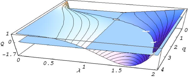
Figure 1. The restriction $Q(\lambda,1,q)$ of the function $Q(\lambda,p,q)$ and the function $O(\lambda,q)\!\equiv\!0$ intersecting along the line $O(1,q)$ and the zero curve $\lambda_{1}(q)$. The oval white mark at the crossing of $O(1,q)$ and $\lambda_{1}(q)$ indicates the location of the golden ratio  $\Phi\!=\!\Phi^{(2)}(1)$. The other white marks indicate the location of the $n$-anacci constants   $\Phi^{(n)}(1)$  with $n\!=\!2,3,4$.

The equation $Q(\lambda,a,q)\!=\!0$, $a\!\in\!\mathbb{R}_{+}$, defines the zero curve $\lambda_{a}(q)$ that contains the sequence of $(m,n)$-anacci constants $\Phi^{(n)}(m)_{n=1}^{\infty}$ if $a\!=\!m$. Next two propositions establish the analytic representation of all zeros of the function $Q(\lambda,p,q)$.

Proposition 2.1.

For any given $p,q\!\in\!\mathbb{R}_{+}$, $p\cdot q\!\neq\!1$, the function $Q(\lambda,p,q)$ of one variable $\lambda$ has the unique zero $\lambda(p,q)\!\neq\!1$, whereas if  $p\cdot q\!=\!1$, its unique zero $\lambda(p,1/p)\!=\!1$. Moreover,

(2.3) $$1<(p+1)q/\!(q+1)<\lambda(p,q)\quad\text{iff}\quad p\cdot q>1;$$

(2.4) $$0<\lambda(p,q)<(p+1)q/\!(q+1)<1\quad\text{iff}\quad p\cdot q<1;$$

(2.5) $$\lambda(p,q)<p+1\quad\text{for any}\quad q\in\mathbb{R}_{+}.$$

Proof.

The partial derivative of function (2.2) with respect to $\lambda$ is given by

(2.6) $$\partial Q(\lambda,p,q)\!/\!\partial\lambda=\lambda^{q-1}\big{(}\lambda(q+1)-(p+1)q\big{)}.$$

Thus, for any $p,q\!\in\!\mathbb{R}_{+}$, the function $Q(\lambda,p,q)$ of the variable $\lambda\!>\!0$ has one local minimum at

(2.7) $$\lambda_{min}(p,q)=(p+1)q/\!(q+1).$$

Formula (2.7) implies that the minimum is assumed at $\lambda_{min}\!=\!1$  iff  $p\cdot q\!=\!1$. In this case, 1 isthe only zero of the function $Q(\lambda,p,q)$ of the variable $\lambda$ because function (2.2) equals zero at $\lambda\!=\!1$, cf. the most left white oval mark  $\Phi^{(1)}(1)\!\!=\!1$  in Fig. 1. If  $p\cdot q\!\neq\!1$, then there must exist a second positive zero  $\lambda(p,q)$ of  $Q(\lambda,p,q)$  besides 1 (if $\lambda_{min}\!<\!1$, the existence of the positive zero is implied by the fact that $Q(0,p,q)\!=p\!>\!0$), cf., Fig. 1. Moreover, the following holds

(2.8) $$1\!<\!\lambda_{min}(p,q)\!<\!\lambda(p,q)\quad\text{iff}\quad p\cdot q\!>\!1\quad\text{and then}\quad Q(\lambda,p,q)\!<\!0\quad\text{iff}\quad 1\!<\!\lambda<\!\lambda(p,q);$$

(2.9) $$0\!<\!\lambda(p,q)\!<\!\lambda_{min}(p,q)\!<\!1\quad\text{iff}\quad p\cdot q\!<\!1\quad\text{and then}\quad Q(\lambda,p,q)\!<\!0\quad\text{iff}\quad\lambda(p,q)\!<\!\lambda\!<\!1;\$$

(2.10) $$\lambda(p,q)\!=\!\lambda_{min}(p,q)\!=\!1\quad\text{iff}\quad p\cdot q\!=\!1\quad\text{and then}\quad Q(\lambda,p,q)\!>\!0\quad\text{iff }\quad\lambda\!\neq\!1.$$

Since $Q(p\!+\!1,p,q)\!=\!p\!>\!0$, formulas (2.8)–(2.10) imply that $\lambda(p,q)\!<\!p\!+\!1$ for any $q\!\in\mathbb{R}_{+}$.

∎

Proposition 2.2.

(i) The assignment $\mathbb{R}_{+}^{2}\!\ni\!(p,q)\to\lambda(p,q)\!\in\!\mathbb{R}_{+}$ defines a continuous function

such that, for any $(p,n)\!\in\!\mathbb{R}_{+}\!\times\!\mathbb{N}$, $\lambda(p,n)\!=\!\lambda^{(n)}(p)$ holds;

1. if $p\cdot q\!\neq\!1$, the function $\lambda(p,q)$ is of class $C^{\infty}$​ and its restriction $\lambda(p,q)|_{\ell}$ to any line  $\ell$ in the domain with the directional angle $0\!\leq\!\alpha\!\leq\!\pi/2$ is strictly increasing;

2. for any $p\!>\!0$ and $q\!\geq\!1$, $p\!\leq\!\lambda(p,q)$, and for any $p\!\in\!\mathbb{R}_{+},$ $\lim_{q\to\infty}\lambda(p,q)=p+1$;

3. for any $p_{0}\!\in\!\mathbb{R}_{+}$, $\lim_{(p,q)\to(p_{0},0)}\!\lambda(p,q)\!=\!0$, and for any $q_{0}\!\in\!\mathbb{R}_{+}$, $\lim_{(p,q)\to(0,q_{0})}\!\lambda(p,q)\!=\!0$, i.e., the open domain ${\mathbb{R}}_{+}^{2}$ of  $\lambda(p,q)$ can be extended to the closed domain $\overline{\mathbb{R}}_{+}^{2}$.

Proof.

(i)  It follows from Proposition 2.1 that the assignment defines a function. If, for $(p_{0},q_{0})$ with $p_{0}\cdot q_{0}\!=\!1$, $\lim_{(p,q)\to(p_{0},q_{0})}\!\lambda(p,q)\!\neq\!1\!=\!\lambda(p_{0},q_{0})$, then we have a contradiction with (2.10) due to the continuity of the function $Q(\lambda,p,q)$ and the fact that $Q\big{(}\lambda(p,q),p,q\big{)}\!=\!0$. Thus, $\lambda(p,q)$ is continuous at $(p_{0},q_{0})$ with $p_{0}\cdot q_{0}\!=\!1$. The continuity of $\lambda(p,q)$ at $(p_{0},q_{0})$ with $p_{0}\cdot q_{0}\!\neq\!1$ is implied by part (ii). The definition of the function $\lambda(p,q)$ assures that $\lambda(p,n)\!=\!\lambda^{(n)}(p)$.

(ii) The equation $Q\big{(}\lambda(p,q),p,q\big{)}\!=\!0$ defines the function $\lambda(p,q)$ implicitly. It follows from formulas (2.6) and (2.7) that the partial derivative $\partial Q(\lambda,p,q)/\partial\lambda$ is continuous and equals 0 iff  $\lambda(p,q)\!=\!\lambda_{min}(p,q)$, i.e., according to (2.10) iff  $p\cdot q\!=\!1$. Thus, the implicit function theorem implies that if  $p\cdot q\!\neq\!1$, the function $\lambda(p,q)$ is continuously differentiable and

(2.11) $$\frac{\partial\lambda(p,q)}{\partial p}=\frac{-1}{\frac{\partial Q\big{(}\lambda(p,q),p,q\big{)}}{\partial\lambda}}\cdot\frac{\partial Q\big{(}\lambda(p,q),p,q\big{)}}{\partial q}=\frac{1-\big{(}\lambda(p,q)\big{)}^{q}}{\left[\lambda(p,q)(q+1)-(p+1)q\right]\big{(}\lambda(p,q)\big{)}^{q-1}},$$

(2.12) $$\frac{\partial\lambda(p,q)}{\partial q}=\frac{-1}{\frac{\partial Q\big{(}\lambda(p,q),p,q\big{)}}{\partial\lambda}}\cdot\frac{\partial Q\big{(}\lambda(p,q),p,q\big{)}}{\partial p}=\frac{\left[p+1-\lambda(p,q)\right]\big{(}\lambda(p,q)\big{)}^{q}\ln q}{\left[\lambda(p,q)(q+1)-(p+1)q\right]\big{(}\lambda(p,q)\big{)}^{q-1}}.$$

Since the function $\lambda(p,q)$ is continuously differentiable if $p\cdot q\!\neq\!1$, it follows from formulas (2.11) and (2.12) that all partial derivatives of $\lambda(p,q)$ of an arbitrary order exist and are continuous. Consequently, the function $\lambda(p,q)$ is of class $C^{\infty}$ if  $p\cdot q\!\neq\!1$.

If $p\cdot q\!>\!1$ (respectively $p\cdot q\!<\!1$), then the denominator and, according to (2.3)–(2.5), both numerators in (2.11) and (2.12) are positive (respectively negative). Thus, the directional derivative of $\lambda(p,q)$ along $\ell$ with the listed property is positive, i.e, $\lambda(p,q)|_{\ell}$ is strictly increasing if $p\cdot q\!\neq\!1$. It follows from Proposition 2.1 that $\lambda(p,q)|_{\ell}$ is also strictly increasing at $p\cdot q\!=\!1$.

(iii) Formula (1.3) implies that  $\lambda(p,1)\!=\!p$, which is smaller than $\lambda(p,q)$, $q\!>\!1$, since for a fixed $p$, $\lambda(p,q)$ is strictly increasing. The convergence to $p\!+\!1$ follows from (2.3) and (2.5).

(iv) The first limit equals 0 due to formulas (2.7) and (2.9). Definition (2.2) implies that the second limit is equal either to 0 or 1. The latter is impossible due to (2.7) and (2.9).

∎

The lower bounds $(p\!+1\!)q/\!(q\!+\!1)$ for $\lambda(p,q)$ in (2.3) predict, e.g., that the golden ratio $\Phi\!\equiv\!\lambda(1,2)$ is only greater than 4/3. The next proposition provides more subtle lower bounds for $\lambda(p,q)$, which imply that the values $\lambda(p,q)$ are close to $p\!+\!1$ already when $q$ is small.

Proposition 2.3.

For any $q\!\geq\!2$ and $p\!>\!1\!/\!\Phi$, it holds

(2.13) $$p+\!1\!-\!1\!/\!(p+\!1)\!<\!\lambda(p,q)$$

moreover, the lower bounds (2.3) and (2.13) satisfy

(2.14) $$(p+1\!)q/\!(q+\!1)\leq p+\!1\!-\!1\!/\!(p+\!1)\quad\text{iff}\quad q\!\leq\!(p+1)^{2}-1.$$

Proof.

Since  $Q^{(2)}_{p}\big{(}p\!+\!1\!-\!1\!/\!(p\!+\!1)\big{)}\!=\!-p(p^{2}\!+\!p\!-1)\!/\!(p\!+\!1)^{2}\!<\!0$  if  $p\!>\!1\!/\!\Phi$, formula (2.8) implies that $p+\!1\!-\!1\!/\!(p+\!1)\!<\!\lambda(p,2)$. Now, for $q\!>\!2$, $\lambda(p,2)\!<\!\lambda(p,q)$ because $\lambda(p,q)$ is strictly increasing for a fixed $p$. Formula (2.14) follows from a simple calculation.

∎

Fig. 2 depicts the restrictions $\lambda(a,q)$ of $\lambda(p,q)$ to the lines $p\!=\!a$, where $a\!=\!\frac{2}{3},1,\dots,2\frac{2}{3}$. Each restriction $\lambda(a,q)$ starts at $\lambda(a,1)\!=\!a$ and increases asymptotically to $a\!+\!1$. It is within the distance $1\!/\!(a\!+\!1)$ from $a\!+\!1$ in the region to the right of the line $q\!=\!2$ (not marked). This lower bound exceeds the lower bound given by formula (2.3) above the white curve $q\!=\!(p\!+\!1)^{2}\!-\!1$ that goes through the points ($3,1)$ and $(4,2\!/\!\Phi)$. The restrictions $\lambda(a,q)$ with an integer $a$ include the $(m,n)$-anacci constants $\Phi^{(n)}(m)$.

Figure 2. The restrictions $\lambda(a,q)$, $a\!=\!\frac{2}{3},1,\dots,2\frac{2}{3}$, $1\!\leq\!q\!\leq\!4$. The white marks indicated the $(m,n)$-anacci constants $\Phi^{(n)}(m)$, $m\!=1,2$, $n\!=\!1,\dots,4$. The white curve $q\!=\!(p\!+\!1)^{2}\!-\!1$

determines the region where the lower bound (2.13) exceeds the lower bound (2.3).

The function $\lambda(p,q)$ is also defined implicitly by the continuous function

(2.15) $$p(\lambda,q)\!\equiv\!\lambda^{q}(\lambda-1)\!/\!(\lambda^{q}-1)\quad\text{if}\quad\lambda\!\neq\!1\quad\text{and}$$

(2.16) $$p(\lambda,q)\!\equiv\!1\!/\!q\quad\text{if}\quad\lambda\!=\!1,$$

which is of class  $C^{\infty}$ if $\lambda\!\neq\!1$.

For $q\!=\!n\!\in\!\mathbb{N}$, the function defined by (2.15)–(2.16) takes the form

(2.17) $$p(\lambda,n)=\frac{\lambda^{n}}{\Sigma_{k=0}^{n-1}\,\lambda^{k}},\quad n\!\in\!\mathbb{N}.$$

Propositions 2.1–2.3 and formula (2.17) imply the following

Corollary 2.4.

(i) The function $\lambda(p,q)$ is concave down where $p\cdot q\!\geq\!1$, i.e., in the sub-domain

of  $\overline{\mathbb{R}}_{+}^{2}$ limited by the hyperbola $p\!\cdot\!q\!=\!1$;

1. the plane $\overline{\mathbb{R}}_{+}^{2}\!\ni(p,q)\!\to\!\mathcal{P}(p,q)\!\equiv\!p\!+\!1$ majorizes the function $\lambda(p,q)$ from above and is the asymptotic plane for $\lambda(p,q)$;

2. the triple $\big{(}\lambda(p,q),p,q\big{)}\!\in\!\mathbb{N}^{3}$ iff it equals $(m,m,\!1)$ with $m\!\in\!\mathbb{N}$, i.e., the $(m,n)$-anacci constants $\Phi^{(n)}(m)$ are integer iff $n\!=\!1$;

3. if the function $\lambda(p,n)\!=\!m\!\in\!\mathbb{N}$ for some $n\!\in\!\mathbb{N}$, then $p$ is rational and $(m\!-\!1)\!<\!p\!<\!m$;

4. the sequences  $\big{(}\Phi^{(n)}(m)\big{)}_{n=1}^{\infty}$ with a fixed $m\!\in\!\mathbb{N}$, $\big{(}\Phi^{(n)}(m)\big{)}_{m=1}^{\infty}$ with a fixed $n\!\in\!\mathbb{N}$, as well as $\big{(}\Phi^{(n)}(kn)\big{)}_{n=1}^{\infty}$ and $\big{(}\Phi^{(km)}(m)\big{)}_{m=1}^{\infty}$ with a fixed $k\!\in\!\mathbb{N}$ are strictly increasing;

5. for any $n\!\in\!\mathbb{N}$, the sequence $\big{(}\frac{m\!+\!1}{m}\Phi^{(n)}(m)\big{)}_{m=1}^{\infty}$ is strictly increasing, cf. Appendix A;

6. if $n\!>\!1$, the sequence $\big{(}\frac{1}{m}\Phi^{(n)}(m)\big{)}_{m=1}^{\infty}$ is strictly decreasing to $1$, cf. Appendix B.

Fig. 3 depicts the asymptotic plane $\mathcal{P}(p,q)\!\equiv\!p+\!1$ and the function $\lambda(p,q)$ generated by using formulas (2.15) and (2.16) in the sub-domain where $0\!\leq\!p\!\leq\!3$ and $0\!\leq\!q\!\leq\!4.1$. The thick curves and the curve at the rim of the graph are the restrictions $\lambda(a,q)$ of $\lambda(p,q)$ with $a\!=\!\frac{1}{3},\frac{2}{3}\dots,2\frac{2}{3},3$. They include the $(m,n)$-anacci constants $\Phi^{(n)}(m)$, $m\!=\!1,2,3$, $n\!=\!1,2,3,4$.

The thin curves increasing from left to right are the restrictions $\lambda(p,q)|_{\ell}$ of $\lambda(p,q)$ to four lines $\ell$ in the domain. These restrictions are not straight lines. Only the restriction to the line $q\!=\!1$, $\lambda(p,1)\!=\!p$, is a straight line. The horizontal thin curves are the level curves $\lambda(p,q)\!=\!c,$ $c\!=\!\frac{1}{2},1\dots,3\frac{1}{2},4$. Among them, only the level curve $\lambda(p,q)\!=\!1$ is a hyperbola.

Figure 3. The function $\lambda(p,q)$ providing the analytic realization of the $(m,n)$-anacci constants and the asymptotic plane $\mathcal{P}(p,q)$ in the sub-domain where $0\!\leq\!p\!\leq\!3$ and $0\!\leq\!q\!\leq\!4.1$. The $\Phi^{(n)}(m)$’s with $m\!=\!1,2,3$ and $n\!=\!1,2,3,4$ lie in the thick curves and the curve at the rim of the graph. The thin curves increasing from left to right are the restrictions $\lambda(p,q)|_{\ell}$ of $\lambda(p,q)$. The horizontal thin curves are the level curves $\lambda(p,q)\!=\!c$ with $c\!=\!\frac{1}{2},1\dots,3\frac{1}{2},4$.

3. Geometric representations of the (m,n)-anacci constants

Let $\Lambda\!\in\!{L}(\mathbb{R}^{n}\!,\mathbb{R}^{n})$ denote a dilation with a dilation factor $\lambda\!>\!0$ acting in the Euclidean space $\mathbb{R}^{n}$ and let $O$ be the homothetic center of the dilation $\Lambda$. Let $\mathfrak{A}\!\subset\!\mathbb{R}^{n}$ be a compact convex $n$-dimensional set with the center of mass $A$. If $O\!\in\!\mathfrak{A}$, then $\mathfrak{A}$ is contained in the image $\Lambda(\mathfrak{A})$ as a proper subset iff $\lambda\!>\!1$, whereas $\Lambda(\mathfrak{A})\!\subsetneq\mathfrak{A}$ iff $0\!<\!\lambda\!<\!1$. Thus, if $\lambda\!>\!1$, we define the non-empty set $\mathfrak{B}\!\equiv\!\Lambda(\mathfrak{A})\!\setminus\!\mathfrak{A}$, and if $0\!<\!\lambda\!<\!1$, we define it as $\mathfrak{B}\!\equiv\mathfrak{A}\mathfrak{\!}\setminus\!\Lambda(\mathfrak{A})$.

We construct geometric representations of the limits $\Phi^{(n)}(p)\!=\!\lambda^{n}(p)$ using dilations of an infinite collection of compact convex sets $\mathfrak{A}(p,n)\!\subset\!\mathbb{R}^{n}\!$, $n\!=1,2,\dots$, and analyzing, for any $p\!\in\!\mathbb{R_{+}}$ and $n\!\in\!\mathbb{N}$, relations among the distances $d(\cdot,\cdot)$ between the following four points in $\mathbb{R}^{n}$:

1. the center of mass $A$ of the set $\mathfrak{A}$ in the collection corresponding to given $p$ and $n$,

2. the homothetic center $O\!\in\!\mathfrak{A}$, $O\!\not=\!A$, of a dilation $\Lambda$ with $\lambda\!>\!0$,

3. the center of mass ${\Lambda(A)}$ of the image $\Lambda(\mathfrak{A})$, and

4. the center of mass $B(\lambda)$ of the set $\mathfrak{B}$.

The centers $O,\,A,\,\Lambda(A)$, and $B(\lambda)$ lie on the line $\mathcal{L}(O,A)$ because the dilations are linear transformations. The set $\mathfrak{B}$ is constructed by removing some mass from the set $\Lambda(\mathfrak{A})$ if $\lambda\!>\!1$ (respectively from $\mathfrak{A}$ if $\lambda\!<\!1$). Thus, the distances satisfy $d(O,A)\!<\!d\big{(}O,\Lambda(A)\big{)}\!<\!d(O,B(\lambda))$ if $\lambda\!>\!1$, cf. Fig. 4, whereas if $\lambda\!<\!1$, $d\big{(}O,\Lambda(A)\big{)}\!<\!d(O,A)\!<\!d(O,B(\lambda))$ holds.

For any $\mathfrak{A}$ and $O$, the function $\big{\{}\mathbb{R}_{+}\!\setminus\!\{1\}\big{\}}\ni\!\lambda\!\to\!B(\lambda)\!\in\!\mathbb{R}^{n}$ is continuous and has its limit at 1 since the function $\mathbb{R}_{+}\!\ni\!\lambda\!\to\!\Lambda(\lambda)\!\in\!{L}(\mathbb{R}^{n}\!,\mathbb{R}^{n})$ is continuous. Thus, we can define the center of mass $B(1)\!\equiv\!\lim_{1\neq\lambda\to 1}B(\lambda)$ despite that the set $\mathfrak{B}$ is not defined if $\lambda\!=\!1$. For a fixed $O$, the center of mass $B(1)$ lies between the centers of mass $A$ and $B(\lambda)$ with $\lambda\!\neq\!1$, cf. Fig. 4.

Figure 4. Dilation with $\lambda\!=\!2.5$ of  $\mathfrak{A}\!\subset\!\mathbb{R}^{2}$ about $O\!\in\!\mathfrak{A}$ resulting in a hollow set $\mathfrak{B}$.

The next proposition provides the basis for constructing uniform geometric representations of the limits $\Phi^{(n)}(p)\!=\!\lambda^{n}(p)$ in terms of the dilation factors $\lambda$. It also determines the position of the center of mass $B(1)$ relative to the center of mass $\Lambda(A)$. In what follows, unless it leads to a confusion, we denote the center of mass $B(\lambda)$ corresponding to a given $\lambda$ just as $B$.

Proposition 3.1.

Let  $\mathfrak{A}\!\subset\!\mathbb{R}^{n}$​ be a compact convex set with the center of mass $A$. Let $\Lambda$ be a dilation about a homothetic center $O\!\in\!\mathfrak{A}$ such that $O\!\not=\!A$, and let $B$ be the center of mass of the set $\mathfrak{B}$. Then the following holds

1. if $\,\lambda\!>\!1$,  then   $\lambda\!=\!\lambda^{(n)}(p)$  iff    $d(A,B)/d(O,A)\!=\!p$  where   $p\!>\frac{1}{n}$,

2. i.e., $\lambda^{(n)}(p)\!=\!d\big{(}O,\Lambda(A)\big{)}/d(O,A);$

3. if  $0\!<\!\lambda\!<\!1$,  then   $\lambda\!=\!1/\lambda^{(n)}(p)$   iff   $d\big{(}\Lambda(A),B\big{)}/d\big{(}O,\Lambda(A)\big{)}\!=\!p$  where  $p\!>\frac{1}{n}$,

4. i.e., $\lambda^{(n)}(p)\!=\!d(O,A)/d\big{(}O,\Lambda(A)\big{)};$

5. if  $\lambda\!=\!1$,  then $\lambda\!=\!\lambda^{(n)}(\frac{1}{n})$   iff    $d\big{(}A,B(1)\big{)}\!=\!d\big{(}\Lambda(A),B(1)\big{)}\!=\!\frac{1}{n}d\big{(}O,A)$.

Proof.

(i) If $\lambda\!>\!1$, the centers of mass are ordered on the line $\mathcal{L}(O,A)$ by their distances from $O$ in the following way: $O\!<\!A\!<\!\Lambda(A)\!<\!B$. Since some mass is removed from $\Lambda(\mathfrak{A})$ to construct the set $\mathfrak{B}$, the location of the center of mass $B$ coincides with the fulcrum of the lever that is in equilibrium when two forces, F_A and F_Λ(A), with magnitudes proportional to the $n$-volumes of the sets $\mathfrak{A}$ and $\Lambda(\mathfrak{A})$, act in opposite directions at $A$ and ${\Lambda(A)}$, respectively.

Dilations with $\lambda\!>\!0$ change distances proportionally to $\lambda$ and $n$-volumes as $\lambda^{n}$, i.e.,

(3.1) $$d(O,{\Lambda(A)})=\lambda d(O,A)\quad{\rm and}\quad$$

(3.2) $${\bf F}_{\Lambda(A)}=-\lambda^{n}{\bf F}_{A}.$$

Using (3.1), we obtain

(3.3) $$d\big{(}{\Lambda(A)},B\big{)}=d(O,A)+d(A,B)-\lambda\,d(O,A),$$

whereas the following equilibrium relation for the lever is implied by (3.2)

(3.4) $$d\big{(}{\Lambda(A)},B\big{)}\lambda^{n}=d(A,B).$$

It follows from relations (3.3) and (3.4) that

(3.5) $$d(A,B)=\lambda^{n}\big{[}d(A,B)+(1-\lambda)d(O,A)\big{]}.$$

In turn, equation (3.5) implies that $\lambda$ is a root of the polynomial

(3.6) $$\lambda^{n+1}-(p+1)\lambda^{n}+p=0,$$

iff  $d(A,B)/d(O,A)\!=\!p$. Since polynomials (2.1) and (3.6) are the same and (3.1) holds, $\lambda\!=\!\lambda^{(n)}(p)\!=\!d\big{(}O,\Lambda(A)\big{)}/d(O,A)$ iff $d(A,B)/d(O,A)\!=\!p$. Formula (2.3) implies that $p\!>\!1/n$.

(ii) If $0\!<\!\lambda\!<\!1$, the centers of mass are ordered by their distances from $O$ as follows: $O\!<\!\Lambda(A)\!<\!A\!<\!B.$ Let us rename the center of mass $\Lambda(A)$ as $A^{\prime}$. Then, $A\!=\!\Lambda^{-1}(A^{\prime})$ where $\Lambda^{-1}$ is the dilation about the homothetic center $O$ with the dilation factor $1/\lambda\!>\!1$.

Part (i) of the proposition implies that $1/\lambda\!=\!\lambda^{(n)}(p)=\!d(O,A)/d\big{(}O,\Lambda(A)\big{)}$ iff $d\big{(}\Lambda(A),B\big{)}/d\big{(}O,\Lambda(A)\big{)}\!=\!p$.

(iii) The claim follows from the definition of $B(1)$ and the fact that $\lambda^{(n)}(p)\!=\!1$ iff $p\!=\!1/n$.

∎

Corollary 3.2.

For a fixed homothetic center $O$, the centers of mass $A$, $\Lambda(A)$, $B(1)$, and $B$ are ordered on the line $\mathcal{L}(O,A)$ by their distances from $O$ in the following way:

1. $O\!<\!A\!<\!B(1)\!<\!\Lambda(A)\!<\!B$    if    $\lambda\!>\!1\!+\!1/n$;

2. $O\!<\!A\!<\!B(1)\!=\!\Lambda(A)\!<\!B$    if    $\lambda\!=\!1\!+\!1/n$;

3. $O\!<\!A\!<\!\Lambda(A)\!<\!B(1)\!<\!B$    if    $1\!<\!\lambda\!<1\!+\!1/n$;

4. $O\!<\!A\!=\!\Lambda(A)\!<\!B(1)\!\leq\!B$    if    $\lambda\!=\!1;$

5. $O\!<\!\Lambda(A)\!<\!A\!<\!B(1)\!<\!B$    if    $0\!<\!\lambda\!<\!1.$

We construct two representations of the $\Phi^{(n)}(m)$’s that have clear geometric interpretations. Replacing $m\!\in\!\mathbb{N}$ by $p\!\in\!\mathbb{R}^{+}\!$ extends the representations to the limits $\Phi^{(n)}(p)$.

First, we use the collection of the unit $n$-balls with the centers of mass at $(1,0,\dots,0)\!\in\!\mathbb{R}^{n}\!$, i.e, the unit $k$-balls with $k\!<\!n$ can be treated as the subsets of the unit $n$-ball. Proposition 3.1 implies that, for any $n$, there exists a dilation about the origin in $\mathbb{R}^{n}$ such that the unit $n$-ball and the dilated $(n\!-\!1)$-sphere enclose the set $\mathfrak{B}(n)$ with the center of mass $B$ positioned at any point in $\mathbb{R}^{n}\!$.

We achieve a clear geometric interpretation of the $n$-anacci constants if, for each $n$, we position the center of mass $B$ uniformly at $(2,0,\dots,0)\!\in\!\mathbb{R}^{n}\!$. Then, the dilated $n$-balls have the radii $\Phi^{(n)}(1)$ and the centers are at $(\Phi^{(n)}(1),0,\dots,0)$.

If $n\!>\!1$, each dilated $n$-ball and the unit $n$-ball form a connected, non-convex set $\mathfrak{B}(n)$ (if $n\!=\!1$, it is a point). The dilated $n$-ball includes all dilated and unit $k$-balls with $k\!<\!n$, and the sets $\mathfrak{B}(n)$ are nested one in the other. Cf. Fig. 5 where $\mathfrak{B}(2)$ has the shape of an eclipsed moon, and the dashed circles with diameters approaching 4 are the projections on $\mathbb{R}^{2}\!$ of the $(n\!-\!1)$-spheres enclosing the sets $\mathfrak{B}(n)$ with $n$=3,4,5.

The $n$-anacci sequence is represented as the centers $\Phi^{(n)}(1)$ of the dilated $n$-balls lying in the interval [1, 2[ at the line $r$e₁, $r\!\in\!\mathbb{R}_{+}$, spanned by the basic vector e₁, as well as the sequence of points $2\,\Phi^{(n)}(1)$ in the interval [2, 4[ where this line intersects the $(n\!-\!1)$-spheres enclosing the sets $\mathfrak{B}(n)$, cf. Fig 5, which depicts, in particular, the constants $2\,\Phi^{(n)}(1)$ with $n\!=\!1,\dots,5$.

This representation can be extended to the $(m,n)$-anacci constants $\Phi^{(n)}(m)$ in the following way. We keep the homothetic center $O$ at the origin in $\mathbb{R}^{n}$ and move the center of mass $B$ to $(m\!+\!1,0,\dots,0)\!\in\!\mathbb{R}^{n}\!,\,m\!\in\!\mathbb{N}$, i.e., we form the collection of connected non-convex (if $n\!>\!1$) sets $\mathfrak{B}(m,n)$, each enclosed by the unit $n$-ball and the dilated $(n\!-\!1)$-sphere with the radius $\Phi^{(n)}(m)$ and the center at $\big{(}\Phi^{(n)}(m),0\dots,0\big{)}$. The inclusion of the dilated and unit $n$-balls as well as the sets $\mathfrak{B}(m,n)$ one in the other follows the order described in the introduction.

The $(m,n)$-anacci constants are represented now by the centers of the dilated $n$-balls $\Phi^{(n)}(m)$ in the intervals $[m,m\!+\!1[$ and as the points $2\,\Phi^{(n)}(m)$ in the intervals $[2\,m,2\,(m\!+\!1)[$ where the $(n\!-\!1)$-spheres enclosing the dilated $n$-balls intersect the first coordinate line $r$e₁.  Fig. 5 depicts the points $2\,\Phi^{(n)}(m)$, $m\!=\!2,3$, $n\!=\!1,\dots,5$, in the intervals [4, 6[ and [6, 8[.

A similar representation of the $\Phi^{(n)}(m)$’s can be obtained using, for instance, the collection of unit $n$-cubes, if the homothetic center $O$ and the center of mass of a face of each unit $n$-cube are located at the origin in $\mathbb{R}^{n}\!$.

Figure 5. Geometric representation of the doubled $(m,n)$-anacci constants $2\,\Phi^{(n)}(m)$ as the points in $\mathbb{R}^{2}\!$ where the dilated $(n\!-\!1)$-spheres intersect the first coordinate line $r{\bf e}_{1}$. The shaded set $\mathfrak{B}(2)\!=\!\mathfrak{B}(1,2)$ as well as the sets $\mathfrak{B}(2,2)$ and $\mathfrak{B}(3,2)$ are enclosed by the unit circle and the solid circles. They all have the shape of eclipsed moons. The dashed circles, intersecting the line $r{\bf e}_{1}$, are the projections on $\mathbb{R}^{2}\!$ of the $(n\!-\!1)$-spheres, which enclose the dilated $n$-balls corresponding to $n\!=\!3,4,5$ and $m\!=\!1,2,3$.

The fact that the center of mass in an $n$-cone divides the interval between the apex and the center of mass of the base according to the ratio $n\!:\!1$, allows us to construct the representation of the $(m,n)$-anacci constants $\Phi^{(n)}(m)$ that has a clear geometric interpretation as well.

Thus, let us consider the collection of regular $n$-cones with the apexes at the origin in $\mathbb{R}^{n}\!,$ the heights equal to 1, and the centers of mass $A(n)$ at $(\frac{n}{n+1},0,\dots,0)\!\in\!\mathbb{R}^{n}\!$. If the radii of the $n$-cones’ spherical bases are all equal, the $k$-cones with $k\!<\!n$ can be treated as the subsets of the $n$-cone.

For any $m,n\!\in\!\mathbb{N}$, we position the homothetic center of a dilation at $\big{(}\frac{m\cdot n-1}{m\cdot(n+1)},0,\dots,0\big{)}\!\in\!\mathbb{R}^{n}\!$, and if $m\!\cdot\!n\!\neq\!1$, we select the dilation factor so that the center of mass $B$ of the set $\mathfrak{B}(m,n)$ is uniformly at $(1,0,\dots,0)\!\in\!\mathbb{R}^{n}\!$, i.e., at the center of mass of the $(n\!-\!1)$-dimensional base of the $n$-cone. If $m\cdot n\!\neq\!1$, the sets $\mathfrak{B}(m,n)$ are hollow, cf. Fig. 6 that depicts the set $\mathfrak{B}(1,2)$

Proposition 3.1 implies that the image of the mass center $A(n)$ under dilation resulting in $B$ at $(1,0,\dots,0)$ is now at the point ($\frac{\Phi^{(n)}(m)+mn-1}{m(n\!+\!1)},0,\dots,0)\!\in\!\mathbb{R}^{n}$ where $\frac{1}{2}\!\leq\!\frac{\Phi^{(n)}(m)+mn-1}{m(n\!+\!1)}\!<\!1$. The $(m,n)$-anacci constants $\Phi^{(n)}(m)$ are represented geometrically by the heights of the dilated $n$-cones in a form of the closed intervals $\big{[}\big{(}1\!-\!\Phi^{(n)}(m)\big{)}\frac{mn-1}{m(n+1)},\big{(}1\!-\!\Phi^{(n)}(m)\big{)}\frac{mn-1}{m(n+1)}\!+\!\Phi^{(n)}(m)\big{]}$ in the line $r$e₁ of the first coordinate.

The ordered nesting of the intervals representing the heights of the dilated $n$-cones holds now only for the sequences $\big{(}\Phi^{(n)}(m)\big{)}_{m=1}^{\infty}$ with a fixed $n\!\in\!\mathbb{N}$, cf. Appendix C. For the sequences $\big{(}\Phi^{(n)}(m)\big{)}_{n=1}^{\infty}$ with a fixed $m\!\in\!\mathbb{N}$, the intervals shift in the negative direction, cf. Fig. 6, which depicts the dilated $2$-cone with the height equal to the golden ratio $\Phi\!=\!\Phi^{(2)}(1)$.

A similar geometric representation of the $(m,n)$-anacci constants $\Phi^{(n)}(m)$ can be constructed using, e.g., the collection of regular $n$-pyramids with the bases consisting of unit $(n\!-\!1)$-cubes, the apexes at the origin in $\mathbb{R}^{n}\!$, the heights equal 1, and the centers of mass at $(\frac{n}{n+1},0,\dots,0)\!\in\!\mathbb{R}^{n}\!$.

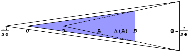
Figure 6. Geometric representation of the golden ratio $\Phi$ by a dilation of the 2-cone.

Interestingly, Proposition 3.1 implies the theorem about the location of the centers of mass in (not-necessarily regular) $n$-cones, $n$-pyramids, and $n$-simplexes. Indeed, if dilations of a set $\mathfrak{A}$ about a fixed homothetic center $O$ result in convex sets $\mathfrak{B}$ for all $\lambda\!\neq\!1$, then $B(\lambda)\!\in\!\mathfrak{B}$ and the center of mass $B(1)$ lies at the intersection of the line $\mathcal{L}(O,A)$ with the boundary of $\mathfrak{A}$.

Moreover, $B(1)$ is the center of mass of the convex part of the boundary of $\mathfrak{A}$, to which the sets $\mathfrak{B}$ are reduced when $\lambda\!\to\!1$. Thus, if we dilate an $n$-dimensional cone, pyramid, or simplex about the homothetic center $O$ positioned at the set’s apex (vertex), then $B(1)$ is the center of mass of the $(n\!-\!1)$-dimensional face opposite to $O$, and Proposition 3.1 implies that the center of mass $A$ of the set $\mathfrak{A}$ divides the distance $d\big{(}O,B(1)\big{)}$ according to the ratio $n\!:\!1$, cf. Fig. 7.

Figure 7. The dilation of a 2-cone with the dilation factor $\lambda\!=\!1.2$ about the apex resulting in a convex set $\mathfrak{B}$. If $\lambda\!\to\!1$, then $B(\lambda)\!\to\!B(1)$ and $\Lambda(A)\!\to\!A$.

The proofs in the Appendices are based on the following facts: $\Phi^{(1)}(m)\!=\!m$, and if $n\!>\!1$,

(3.7) $$m\!+\!1\!-\!1\!/\!(m+1)\!<\!\Phi^{(n)}(m)\!<\!m\!+\!1.$$

4. Appendix A. Proof of Corollary 2.4 (vi)

If $n\!=\!1$, the sequence $\big{(}\!\frac{m+1}{m}\Phi^{(1)}(m)\!\big{)}_{\!m=1}^{\!\infty}\!$ is strictly increasing since $m+1\!\leq\!m+2$. If $n\!>\!1$, (3.7) implies that $\frac{m+1}{m}\Phi^{(n)}(m)\!<\!\frac{(m+1)^{2}}{m}\!\leq\!\frac{m+2}{m+1}\big{(}m+2\!-\!\frac{1}{(m+2)}\big{)}\!<\!\frac{m\!+\!2}{m\!+\!1}\,\Phi^{(n)}(m\!+\!1)$ is true for any $m$.

5. Appendix B. Proof of Corollary 2.4 (vii)

If $n\!=\!1$, $\frac{1}{m}\Phi^{(1)}(m)\!=\!1$ for any $m$. If $n\!>\!1$, the sequence $\big{(}\frac{1}{m}\Phi^{(n)}(m)\big{)}_{\!m=1}^{\!\infty}$ is strictly decreasing to $1$ since (3.7) implies that $\frac{m+2}{m+1}\!-\!\frac{1}{(m+2)(m+1)}\!<\!\frac{\Phi(m+1)}{m+1}\!<\!\frac{m+2}{m+1}\!\leq\!\big{(}m\!+\!1\!-\!\frac{1}{(m+1)}\big{)}\!<\!\frac{\Phi(m)}{m}\!<\!1\!+\!\frac{1}{m}$ where the middle inequality reduces to $m\!>\!1\!/\!\Phi$.

6. Appendix C. Proof of the nesting of the heights representing the (m,n)-anacci constants

For a fixed $n\!=\!1$, the nesting of the left ends of the intervals, which is consistent with the introduced order, is implied by the fact that $-\frac{m^{2}}{2(m+1)}\!<\!-\frac{(m-1)^{2}}{2m}$  iff  $m\!>\!1\!/\!\Phi$. For $n\!>\!1$, formula (3.7) implies that $\big{(}1\!-\!\Phi^{(n)}(m\!+\!1)\big{)}\frac{(m+1)n-1}{(m+1)(n+1)}\!<\!\frac{1-(m+1)(m+2)}{(m+2)}\cdot\frac{(m+1)n-1}{(m+1)(n+1)})\!\leq\!-m\frac{mn-1}{m(n+1)}\!<\!\big{(}1\!-\!\Phi^{(n)}(m)\big{)}\frac{mn-1}{m(n+1)}$ is true (the middle inequality is equivalent to $-(nm^{2}\!+\!2mn\!+\!n\!+\!1)\!\leq\!0$).

The nesting of the right ends follows from $\frac{m+1}{m}\Phi^{(n)}(m)\!<\!\frac{m+2}{m+1}\Phi^{(n)}(m\!+\!1)$, which is true for any $n$ due to Corollary 2.4 (vi), and from $\frac{mn-1}{m}\!<\!\frac{(m+1)n-1}{m+1}$, which holds for any $m$ and $n$.

MSC2010: 40A05, 40A30, 40B05

References

[1]
P. F. Byrd,
Problem H-61, The Fibonacci Quarterly, 3.3 (1965), 201. Solution, The Fibonacci Quarterly,
5.1 (1967), 72.
[2] H, S. M. Coxeter, Regular Polytopes, Dover Publications 1973, third edition.
[3]
F. Dubeau,
On r-Generalized Fibonacci Numbers, The Fibonacci Quarterly, 27.3 (1989), 221–228.
[4]
F. Dubeau et al.,
On Weighted r-Generalized Fibonacci Sequences, The Fibonacci Quarterly, 35.2 (1997), 102–110.
[5]
I. Flores,
Direct Calculation of k-Generalized Fibonacci Numbers, The Fibonacci Quarterly, 5.3 (1967), 259–268.
[6]
A. F. Horadam,
A Generalized Fibonacci Sequence, Amer. Math. Monthly, 68.5 (1961), 455–59.
[7]
A. F. Horadam,
Basic Properties of a Certain Generalized Sequence of Numbers, The Fibonacci Quarterly, 3.3 (1965), 161–176.
[8] T. Khovanova, Recursive Sequences,
http://www.tanyakhovanova.com/RecursiveSequences/RecursiveSequences.html
[9] A. M. Ostrowski,
Solutions of Equations and Systems of Equations, Academic Press 1966, second edition.
[10]
OEIS Foundation Inc. (2011), The On-Line Encyclopedia of Integer Sequences,
http://oeis.org/wiki/Index_to_OEIS:_Section_Rec
[11]
L. Somer. Problem H-197 and solution, The Fibonacci Quarterly, 12.1 (1974), 110–111.