Kolmogorov structure functions for automatic complexity

Abstract

For a finite word $w$ we define and study the Kolmogorov structure function $h_{w}$ for nondeterministic automatic complexity. We prove upper bounds on $h_{w}$ that appear to be quite sharp, based on numerical evidence.

1 Introduction

Shallit and Wang [4] introduced automatic complexity as a computable alternative to Kolmogorov complexity. They considered deterministic automata, whereas Hyde and Kjos-Hanssen [3] studied the nondeterministic case, which in some ways behaves better. Unfortunately, even nondeterministic automatic complexity is somewhat inadequate. The string $00010000$ has maximal nondeterministic complexity, even though intuitively it is quite simple. One way to remedy this situation is to consider a structure function analogous to that for Kolmogorov complexity.

The latter was introduced by Kolmogorov at a 1973 meeting in Tallinn and studied by Vereshchagin and Vitányi [6] and Staiger [5].

Figure 1: A nondeterministic finite automaton that only accepts one string $x=x_{1}x_{2}x_{3}x_{4}\ldots x_{n}$ of length $n=2m+1$.

The Kolmogorov complexity of a finite word $w$ is roughly speaking the length of the shortest description $w^{*}$ of $w$ in a fixed formal language. The description $w^{*}$ can be thought of as an optimally compressed version of $w$. Motivated by the non-computability of Kolmogorov complexity, Shallit and Wang studied a deterministic finite automaton analogue.

Definition 1 (Shallit and Wang [4]).

The automatic complexity of a finite binary string $x=x_{1}\dots x_{n}$ is the least number $A_{D}(x)$ of states of a deterministic finite automaton $M$ such that $x$ is the only string of length $n$ in the language accepted by $M$.

Hyde and Kjos-Hanssen [3] defined a nondeterministic analogue:

Definition 2.

The nondeterministic automatic complexity $A_{N}(w)$ of a word $w$ is the minimum number of states of an NFA $M$, having no $\epsilon$-transitions, accepting $w$ such that there is only one accepting path in $M$ of length $\lvert w\rvert$.

The minimum complexity $A_{N}(w)=1$ is only achieved by words of the form $a^{n}$ where $a$ is a single letter.

Definition 3.

Let $n=2m+1$ be a positive odd number, $m\geq 0$. A finite automaton of the form given in Figure 1 for some choice of symbols $x_{1},\dots,x_{n}$ and states $q_{1},\dots,q_{m+1}$ is called a Kayleigh graph.

Theorem 4 (Hyde [2]).

The nondeterministic automatic complexity $A_{N}(x)$ of a string $x$ of length $n$ satisfies

$$A_{N}(x)\leq b(n):={\lfloor}n/2{\rfloor}+1\text{.}$$

Proof.

If $n$ is odd, then a Kayleigh graph witnesses this inequality. If $n$ is even, a slight modification suffices, see [2]. ∎

The structure function of a string $x$ is defined by $h_{x}(m)=\min\{k:$ there is a $k$-state NFA $M$ which accepts at most $2^{m}$ strings of length $\lvert x\rvert$ including $x\}$. In more detail:

Let

$$S_{x}=\{(q,m)\mid\exists\text{ $q$-state NFA $M$},x\in L(M)\cap\Sigma^{n},\lvert L(M)\cap\Sigma^{n}\rvert\leq b^{m}\}.$$

Then $S_{x}$ has the upward closure property

$$q\leq q^{\prime},m\leq m^{\prime},(q,m)\in S_{x}\quad\Longrightarrow\quad(q^{\prime},m^{\prime})\in S_{x}.$$

From $S_{x}$ we can define the structure function $h_{x}$ and the dual structure function $h_{x}^{*}$.

Definition 5 (Vereshchagin, personal communication, 2014, inspired by [6]).

In an alphabet $\Sigma$ containing $b$ symbols, we define

$$h^{*}_{x}(m)=\min\{k:(k,m)\in S_{x}\}\quad\text{and}$$

$$h_{x}(k)=\min\{m:(k,m)\in S_{x}\}.$$

Remark 6.

On the one hand, $h$ mimics the structure function as defined by Kolmogorov. On the other hand, $h^{*}$ has a natural domain $[0,n]$ whereas the domain of $h$ is initially $[1,\infty)$, until some upper bound on the automatic complexity is proved, at which point it becomes $[1,\lfloor n/2\rfloor+1]$. One often prefers that a function have a simple domain and a complicated range rather than the other way around, e.g., consider the case of the range of a computable function on $\mathbb{N}$ (which is only computably enumerable).

History of the structure function.

Kolmogorov first introduced the structure function in a talk at The Third International Symposium on Information Theory, June 18–23, 1973, Tallinn, Estonia, Soviet Union. The meeting coincided with a Nixon/Brezhnev meeting in the U.S. Kolmogorov was born in 1903 hence 70 years old at the time. The results were not published until they appeared as an abstract of a talk for the Moscow Mathematical Society [1] in Uspekhi Mat. Nauk in the Communications of the Moscow Mathematical Society, page 155 (in the Russian edition, not translated into English). The talk was given on April 16, 1974 and was entitled “Complexity of algorithms and objective definition of randomness”.

2 Basic properties

Definition 7.

The entropy function $\mathcal{H}:[0,1]\rightarrow[0,1]$ is given by

$$\mathcal{H}(p)=-p\log_{2}p-(1-p)\log_{2}(1-p).$$

Remark 8.

Throughout the paper, $\log$ (with no subscript) denotes either the natural logarithm $\ln=\log_{e}$, or $\log_{b}$ where the value of $b$ is immaterial.

Theorem 9.

For $0\leq k\leq n$,

$$\log_{2}{n\choose k}=\mathcal{H}(k/n)n+O(\log n).$$

Proof.

For $u\in\mathbb{N}$, let

$$S_{u}=\sum_{k=2}^{u}\log k,\quad I_{u}=\int_{1}^{u}\log x\,dx,\quad\text{and}\quad J_{u}=\int_{2}^{u+1}\log x\,dx.$$

Let

$$\alpha_{n}=\log{n\choose k}=S_{n}-S_{k}-S_{n-k}.$$

Note $I_{u}\leq S_{u}\leq J_{u}$ and

$$J_{u}-I_{u}=\int_{u}^{u+1}\log x\,dx-\int_{1}^{2}\log x\,dx\leq\log(u+1),$$

Thus up to $O(\log n)$ error terms we have

$$\alpha_{n}=\int^{n}_{1}\log x\,dx-\int_{1}^{k}\log x\,dx-\int_{1}^{n-k}\log x\,dx$$

$$=(n\log n-n)-(k\log(k)-k)-[(n-k)\log(n-k)-(n-k)]$$

$$=n\log n-k\log(k)-(n-k)\log(n-k)$$

$$=-k\log(k/n)-(n-k)\log\left(1-\frac{k}{n}\right)$$

and hence

$$\log_{2}{n\choose k}=-k\log_{2}(k/n)-(n-k)\log_{2}(1-k/n)=\mathcal{H}(k/n)\cdot n.$$

∎

Figure 2: An automaton illustrating multi-run complexity for a string of length $n$ containing $m$ many 0s, and $n-m$ many 1s.

Theorem 10.

Suppose the number of $0$s in the binary string $x$ is $p\cdot n$. Then

$$h^{*}_{x}(\mathcal{H}(p)n)\leq pn+O(\log n).$$

Proof.

Consider an automaton $M$ as in Figure 2 that has $p\cdot n$ many states, and that has one left-to-right arrow labeled 0 for each 0, and a loop in place labeled 1 for each consecutive string of 1s. Since $M$ accepts exactly those strings that have $p\cdot n$ many 0s, the number of strings accepted by $M$ is ${n\choose p\cdot n}$. By Theorem 9 this is $\leq 2^{k}$ approximately when $\mathcal{H}(p)n\leq k$, and we are done. ∎

Example 11.

A string of the form $0^{a}1^{n-a}$ satisfies $h^{*}_{x}(\log_{2}n)=2$ whereas $h^{*}_{x}(0)$ may be $n/2$. For instance $0011$ has $h^{*}_{x}(2)=2$. On the other hand $h^{*}_{x}(1)=3$ which is why this string is more complicated than $0110$.

Figure 3: An automaton illustrating the linear upper bound on the automatic structure function from Theorem 12.

Theorem 12.

For any $x$ of length $n$,

$$1\leq h^{*}_{x}(m)\leq n-m+1\text{ for }0\leq m\leq n.$$

Proof.

$1\leq h^{*}_{x}(n-k)\leq k+1$ because we can start out with a sequence of determined moves, after which we accept everything, as in Figure 3. ∎

3 Upper bounds on structure function for automatic complexity

Definition 13.

The dual automatic structure function of a string $x$ of length $n$ is a function $h^{*}_{x}:[0,n]\rightarrow[0,\lfloor n/2\rfloor+1]$. We define the asymptotic upper envelope of $h^{*}$ by

$$\widetilde{h^{*}}(a)=\limsup_{n\rightarrow\infty}\max_{\lvert x\rvert=n}\frac{h^{*}_{x}([a\cdot n])}{n},\quad\widetilde{h^{*}}:[0,1]\rightarrow[0,1/2]$$

where $[\cdot]$ is the nearest integer function. Let

$$\tilde{h}(p)=\limsup_{n\rightarrow\infty}\max_{\lvert x\rvert=n}\frac{h_{x}([p\cdot n])}{n},\quad\tilde{h}:[0,1/2]\rightarrow[0,1].$$

Theorem 14 (Main Theorem).

Assume $x$ is a binary string, so the alphabet size $b=2$. The asymptotic upper envelope $\tilde{h}$ of the automatic structure functions $h_{x}$ satisfies

$$\tilde{h}(p)\leq\psi(p):=\begin{cases}\mathcal{H}(\frac{1}{2}-p),&\frac{\sqrt{3}}{4}\leq p\leq\frac{1}{2},\\ 2-\alpha p,&\frac{1}{\alpha-1}\leq p\leq\frac{\sqrt{3}}{4},\\ 1-p,&0\leq p\leq\frac{1}{\alpha-1},\end{cases}$$

where

$$\alpha=\frac{4}{\sqrt{3}}\left(2-\mathcal{H}\left(\frac{1}{2}-\frac{\sqrt{3}}{4}\right)\right)=\mathcal{H}^{\prime}\left(\frac{1}{2}-\frac{\sqrt{3}}{4}\right)\approx 3.79994,$$

$$\alpha=2\log_{2}(2+\sqrt{3}).$$

As Theorem 14 shows, the largest number of paths is obtained by going fairly straight to the loop state; spending half the time looping and half the time meandering; and then finally going equally fairly straight to the start state. The optimal value of $r$ obtained shows that half of the time between first reaching the loop state and finally leaving the loop state should be spent looping. Figures 4 and 5 show our upper bounds for the automatic structure function.

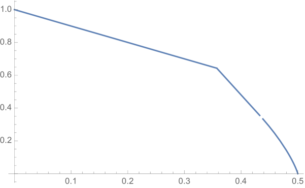
Figure 4: Bounds for the automatic structure function for alphabet size $b=2$ when $\vec{c}=(1,-1,0)$; see Theorem 14. Figure produced using Mathematica with $y=\min\left(2-{2\log_{2}(2+\sqrt{3})}x,1-x\right)$ for $0\leq x\leq\frac{\sqrt{3}}{4}$, and $y={-(\frac{1}{2}-x)\log_{2}(\frac{1}{2}-x)-(\frac{1}{2}+x)\log_{2}(\frac{1}{2}+x)}$ for $\frac{\sqrt{3}}{4}\leq x$.

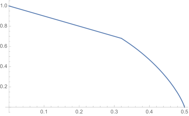
Figure 5: Bounds for the automatic structure function for alphabet size $b=2$; see Theorem 14. When $\vec{c}=\frac{1}{2}(1,-1,1)$, the entropy function is used on $[0.33,0.5]$, the tangent line on $[0.3205,0.330]$, and $y=1-x$ on $[0,0.3205]$. Figure produced using Mathematica with $y=\min(\sqrt{2}-2.29244x,1-x)$ for $0\leq x<0.330$, and $y={-(\frac{1}{2}-x)\log_{2}(\frac{1}{2}-x)-(\frac{1}{2}+x)\log_{2}(\frac{1}{2}+x)}$ for $0.330\leq x$.

4 Proof of Theorem 14

Consider a path of length $n$ through a Kayleigh graph with $q=pn$ many states. Let $t_{1}$ be the time spent before reaching the loop state for the first time. Let $t_{2}$ be the time spent after leaving the loop state for the last time. Let $s$ be the number of self-loops taken by the path. Let us say that meandering is the process of leaving the loop state after having gone through a loop, and before again going through a loop. For fixed $p$ let

$$\gamma(t_{1},t_{2},s,n)={t_{1}\choose\frac{t_{1}-pn}{2}}{t_{2}\choose\frac{t_{2}-pn}{2}}{\chi(n,t,s)\choose s}{\chi(n,t,s)-s\choose\frac{\chi(n,t,s)-s}{2}}b^{s}$$

where $\chi(n,t,s)=n-t$ and $t=t_{1}+t_{2}$. (By Lemma 15, we can also let $\chi(n,t,s)=(n-t+s)/2$, since the number of non-loops between loops must be even. This gives a better upper bound.)

Then the number of such paths is

$$N\leq\sum_{s}\sum_{t_{1}}\sum_{t_{2}}\gamma(t_{1},t_{2},s,n)$$ (1)

since half of the meandering times must be backtrack times.

Lemma 15.

Suppose $0\leq k\leq n$ with $n-k$ even. The number of $k$-element subsets of $\{1,\dots,n\}$ where the number of other elements between consecutive elements in the subset is always even is

$${(n-k)/2+k\choose k}.$$

Proof.

The other elements come in pairs hence by merging the pair to one there are only $(n-k)/2$ of them. ∎

For instance, if $n=6$ and $k=2$, we get ${4\choose 2}=6$. Since

$$\limsup_{n\rightarrow\infty}\frac{\log_{b}\sum_{1}^{n}a_{i}}{n}\leq\limsup_{n\rightarrow\infty}\frac{\log_{b}(n\cdot\max a_{i})}{n}=\limsup_{n\rightarrow\infty}\frac{\log_{b}\max a_{i}}{n},$$

the sums can be replaced by maxima, i.e.,

$$\limsup_{n\rightarrow\infty}\frac{\log_{b}N}{n}\leq\limsup_{n\rightarrow\infty}\frac{\log_{b}\gamma(t_{1},t_{2},s,n)}{n},\quad(t_{1},t_{2},s)\in\operatorname*{arg\,max}_{(t_{1},t_{2},s)}\gamma(t_{1},t_{2},s,n).$$

By Theorem 9,

$$\limsup_{n\rightarrow\infty}\frac{\gamma(t_{1},t_{2},s,n)}{n}\leq\limsup_{n\rightarrow\infty}\frac{\delta(t_{1},t_{2},s,n)}{n}$$

where $\delta$ is

$$\sum_{i=1}^{2}t_{i}\mathcal{H}_{b}\left(\frac{1}{2}-\frac{pn}{2t_{i}}\right)+\left(\chi(n,t,s)\right)\mathcal{H}_{b}\left(\frac{s}{\chi(n,t,s)}\right)+ \left(\chi(n,t,s)-s\right)\mathcal{H}_{b}\left(\frac{1}{2}\right)+s$$

$$=\sum_{i=1}^{2}t_{i}\mathcal{H}_{b}\left(\frac{1}{2}-\frac{pn}{2t_{i}}\right)+\left(\chi(n,t,s)\right)\mathcal{H}_{b}\left(\frac{s}{\chi(n,t,s)}\right)+ \chi(n,t,s)\log_{b}2+(1-\log_{b}2)s,$$

where $\mathcal{H}_{b}=\mathcal{H}/\log_{2}b$ and $t=t_{1}+t_{2}$. Note that $\mathcal{H}_{b}(1/2)=1/\log_{2}b$. Now let $\Delta(T_{1},T_{2},r)=\delta(T_{1}n,T_{2}n,rn,n)/n$ for any $n$. It does not matter which $n$, since with $T=T_{1}+T_{2}$, $\chi(n,t,s)=c_{\mathrm{n}}n+c_{\mathrm{t}}t+c_{\mathrm{s}}s$ gives

$$\frac{1}{n}\chi(n,Tn,rn)=c_{\mathrm{n}}+c_{\mathrm{t}}T+c_{\mathrm{s}}r$$

and

$$\frac{rn}{\chi(n,Tn,rn)}=\frac{r}{c_{\mathrm{n}}+c_{\mathrm{t}}T+c_{\mathrm{s}}r}$$

and hence $\Delta(T_{1},T_{2},r)$ equals

$$\sum_{i=1}^{2}T_{i}\mathcal{H}_{b}\left(\frac{1}{2}-\frac{p}{2T_{i}}\right)+(c_{\mathrm{n}}+c_{\mathrm{t}}T+c_{\mathrm{s}}r)\mathcal{H}_{b}\left(\frac{r}{c_{\mathrm{n}}+c_{\mathrm{t}}T+c_{\mathrm{s}}r}\right)$$

$$+\left(c_{\mathrm{n}}+c_{\mathrm{t}}T+c_{\mathrm{s}}r\right)\log_{b}2+(1-1/\log_{2}b)r.$$

Lemma 16.

$\Delta(T_{1},T_{2},r)$ is maximized at $T_{1}=T_{2}$.

Proof.

Rewriting with $T=T_{1}+T_{2}$ and $\epsilon=T_{1}-T_{2}$, it suffices to show that with $g(x)=x\mathcal{H}(1/2-1/x)$, the function $f(\epsilon)=g(x+\epsilon)+g(x-\epsilon)$ is maximized at $\epsilon=0$. This is equivalently to $g$ being concave, which is a routine verification:

$$g^{\prime}(x)=\mathcal{H}(1/2-1/x)+x\mathcal{H}^{\prime}(1/2-1/x)(1/x^{2})=\mathcal{H}(1/2-1/x)+\mathcal{H}^{\prime}(1/2-1/x)/x$$

$$g^{\prime\prime}(x)=\mathcal{H}^{\prime}(1/2-1/x)/x^{2}+\mathcal{H}^{\prime\prime}(1/2-1/x)(1/x^{2})(1/x)+\mathcal{H}^{\prime}(1/2-1/x)(-1/x^{2})$$

$$g^{\prime\prime}(x)=\mathcal{H}^{\prime\prime}(1/2-1/x)/x^{3}<0$$

∎

Definition 17 (Logit function).

For any real $b>1$,

$$\operatorname{logit}_{b}(x)=\log_{b}\left(\frac{x}{1-x}\right),\quad\operatorname{logit}_{b}:(0,1)\rightarrow\mathbb{R}.$$

A graphic of the logit function is given as Figure 6.

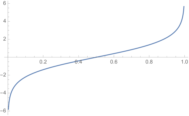
Figure 6: The logit function for $b=e$. Figure produced using Mathematica with $y=\log\left(\frac{x}{1-x}\right)$.

Definition 18 (Logistic sigmoid function).

For any real $b>1$,

$$\zeta_{b}(y)=\frac{1}{b^{-y}+1},\quad\zeta_{b}:\mathbb{R}\rightarrow(0,1).$$

Lemma 19.

For any real $b>1$, the logit function $\operatorname{logit}_{b}(x)$ is a strictly increasing bijection. Its inverse is the logistic sigmoid function $\zeta_{b}(y)$.

In light of Lemma 16, we now let $\Delta(T,r)=\Delta(T/2,T/2,r)$, so that

$$\Delta(T,r)=T\mathcal{H}_{b}\left(\frac{1}{2}-\frac{p}{T}\right)+(c_{\mathrm{n}}+c_{\mathrm{t}}T+c_{\mathrm{s}}r)\mathcal{H}_{b}\left(\frac{r}{c_{\mathrm{n}}+c_{\mathrm{t}}T+c_{\mathrm{s}}r}\right)$$

$$+(c_{\mathrm{n}}+c_{\mathrm{t}}T+c_{\mathrm{s}}r)\log_{b}2+(1-\log_{b}2)r.$$

In the following Lemma it is useful to have the default case $(c_{\mathrm{n}},c_{\mathrm{t}},c_{\mathrm{s}})=(1,-1,0)$. The other case of interest is $(c_{\mathrm{n}},c_{\mathrm{t}},c_{\mathrm{s}})=(1/2,-1/2,1/2)$.

Lemma 20.

For fixed $p$, $b$, and $T$, the function $r\mapsto\Delta(T,r)$ has a unique maximum where

$$r=(c_{\mathrm{n}}+c_{\mathrm{t}}T+c_{\mathrm{s}}r)\frac{b}{b+2^{1-c_{\textrm{s}}}},$$

hence after optimizing on $r$, $\Delta(T)-T\mathcal{H}_{b}\left(\frac{1}{2}-\frac{p}{T}\right)=$

$$(c_{\mathrm{n}}+c_{\mathrm{t}}T+c_{\mathrm{s}}r)\mathcal{H}_{b}\left(\frac{b}{b+2^{1-c_{\textrm{s}}}}\right)+(c_{\mathrm{n}}+c_{\mathrm{t}}T+c_{\mathrm{s}}r)\log_{b}2$$

$$+(1-\log_{b}2)\left[(c_{\mathrm{n}}+c_{\mathrm{t}}T+c_{\mathrm{s}}r)\frac{b}{b+2^{1-c_{\textrm{s}}}}\right],$$

i.e.,

$$\Delta(T)=T\mathcal{H}_{b}\left(\frac{1}{2}-\frac{p}{T}\right)+(c_{\mathrm{n}}+c_{\mathrm{t}}T+c_{\mathrm{s}}r)\underbrace{\left\{\mathcal{H}_{b}\left(\frac{b}{b+2^{1-c_{\textrm{s}}}}\right)+\log_{b}2+(1-\log_{b}2)\left[\frac{b}{b+2^{1-c_{\textrm{s}}}}\right]\right\}}_{c_{b}:=}$$

$$=T\mathcal{H}_{b}\left(\frac{1}{2}-\frac{p}{T}\right)+\frac{(c_{\mathrm{n}}+c_{\mathrm{t}}T)}{\left(1-c_{\mathrm{s}}\frac{b}{b+2^{1-c_{\textrm{s}}}}\right)}c_{b}$$

$$=T\mathcal{H}_{b}\left(\frac{1}{2}-\frac{p}{T}\right)+(1-T)\underbrace{\frac{c_{\mathrm{n}}c_{b}}{\left(1-c_{\mathrm{s}}\frac{b}{b+2^{1-c_{\textrm{s}}}}\right)}}_{d_{b}}\quad\text{if }c_{\mathrm{n}}=-c_{\mathrm{t}}.$$

namely

$$r=\frac{(c_{\mathrm{n}}+c_{\mathrm{t}}T)\frac{b}{b+2^{1-c_{\textrm{s}}}}}{\left(1-c_{\mathrm{s}}\frac{b}{b+2^{1-c_{\textrm{s}}}}\right)}=\frac{c_{\mathrm{n}}+c_{\mathrm{t}}T}{\left(\frac{b+2^{1-c_{\textrm{s}}}}{b}-c_{\mathrm{s}}\right)}$$

$$=\begin{cases}(1-T)\frac{b}{b+2},&(c_{\mathrm{n}},c_{\mathrm{t}},c_{\mathrm{s}})=(1,-1,0)\\ \frac{1}{2}(1-T)/(\frac{b+\sqrt{2}}{b}-\frac{1}{2}),&(c_{\mathrm{n}},c_{\mathrm{t}},c_{\mathrm{s}})=(1/2,-1/2,1/2)\end{cases}$$

Proof.

We have

$$\frac{d}{dx}\mathcal{H}_{b}(x)=-\operatorname{logit}_{b}(x).$$

Thus by Lemma 19, the inverse function of $\mathcal{H}_{b}^{\prime}(x)$ is $y\mapsto\zeta_{b}(-y)=\frac{1}{b^{y}+1}$. Thus, we calculate

$$\frac{\partial\Delta}{\partial r}=\mathcal{H}_{b}^{\prime}(r/(c_{\mathrm{n}}+c_{\mathrm{t}}T+c_{\mathrm{s}}r))+1-\log_{b}2+c_{\mathrm{s}}\log_{b}2=0\quad\text{iff}$$

$$\frac{r}{c_{\mathrm{n}}+c_{\mathrm{t}}T+c_{\mathrm{s}}r}=(\mathcal{H}_{b}^{\prime})^{-1}(\log_{b}2-1-c_{\mathrm{s}}\log_{b}2)=\frac{1}{b^{\log_{b}2-1-c_{\mathrm{s}}\log_{b}2}+1}$$

$$=\frac{1}{\frac{2^{1-c_{\mathrm{s}}}}{b}+1}=\frac{b}{b+2^{1-c_{\textrm{s}}}},$$

as desired. We also have

$$\frac{d}{dx}\operatorname{logit}_{b}(x)=\frac{1}{\ln b}\cdot\frac{1}{x(1-x)}.$$

Note that if $(c_{\mathrm{n}},c_{\mathrm{t}},c_{\mathrm{s}})=(1,-1,0)$ then $T<1$ gives $r>0$. Hence

$$\frac{\partial^{2}\Delta}{\partial r^{2}}=\frac{\partial}{\partial r}\left(-\operatorname{logit}_{b}\left(\frac{r}{c_{\mathrm{n}}+c_{\mathrm{t}}T+c_{\mathrm{s}}r}\right)\right)$$

$$=(-1)\frac{\partial}{\partial r}\left(\frac{r}{c_{\mathrm{n}}+c_{\mathrm{t}}T+c_{\mathrm{s}}r}\right)\cdot\frac{1}{\ln(b)}\cdot\frac{1}{x(1-x)}\bigg{\rvert}_{x=\frac{r}{c_{\mathrm{n}}+c_{\mathrm{t}}T+c_{\mathrm{s}}r}}$$

$$=(-1)\left(\frac{c_{\mathrm{n}}+c_{\mathrm{t}}T+c_{\mathrm{s}}r-rc_{\mathrm{s}}}{(c_{\mathrm{n}}+c_{\mathrm{t}}T+c_{\mathrm{s}}r)^{2}}\right)\cdot\frac{1}{\ln(b)}\cdot\frac{1}{x(1-x)}\bigg{\rvert}_{x=\frac{r}{c_{\mathrm{n}}+c_{\mathrm{t}}T+c_{\mathrm{s}}r}}<0$$

provided $c_{\mathrm{t}}=-c_{\mathrm{n}}<0$ and $c_{\mathrm{s}}>0$, as in our two cases. ∎

In light of Lemma 20, we now let $r=(1-T)\frac{b}{b+2}$ in $\Delta(T,r)=\Delta(T/2,T/2,r)$, giving

$$\varphi(T,p):=T\mathcal{H}_{b}\left(\frac{1}{2}-\frac{p}{T}\right)+(1-T)\mathcal{H}_{b}\left(\frac{r}{1-T}\right)+(1-T)\log_{b}2+(1-\log_{b}2)r$$

$$=T\mathcal{H}_{b}\left(\frac{1}{2}-\frac{p}{T}\right)+(1-T)\mathcal{H}_{b}\left(\frac{b}{b+2}\right)+(1-T)\log_{b}2+(1-\log_{b}2)(1-T)\frac{b}{b+2}$$

which we will call $\varphi(T,p)$.

To simplify calculations to come, we make Definition 21.

Definition 21 (Abbreviations).

$$T(p) :=\frac{2p}{\sqrt{1-\frac{4}{(b+2)^{2}}}}=\frac{4p}{\sqrt{3}},\quad b=2.$$

$$\varphi(T,p) :=\Delta\left(T,(1-T)\frac{b}{b+2}\right)$$

$$\beta(T) :=\frac{1}{2}-\frac{p}{T}.$$

Note that $\alpha_{2}=\frac{2\cosh^{-1}(2)}{\ln 2}=2\log_{2}(2+\sqrt{3})$. Then

$$\lim_{n\rightarrow\infty}\frac{\log_{2}N}{n}\leq\varphi(T,p)=T\mathcal{H}_{b}\left(\beta(T)\right)+(1-T)c_{b}.$$

Lemma 22.

Suppose $0\leq 2p\leq T\leq 1$ and $b\geq 2$. Suppose

$$\varphi(T,p)=T\mathcal{H}_{b}\left(\beta(T)\right)+(1-T)d_{b}.$$

for some constant $d_{b}$. Then we have

$$0<\frac{\partial\varphi}{\partial T}\quad\Longleftrightarrow\quad T<T(p)$$

where $T(p)=\frac{2}{\sqrt{1-4b^{-2d_{b}}}}p$.

Proof.

We have, using the further abbreviation $\beta=\beta(T)$,

$$\frac{\partial\varphi}{\partial T}=\mathcal{H}_{b}\left(\beta\right)+T\mathcal{H}_{b}^{\prime}\left(\beta\right)\cdot\frac{p}{T^{2}}-d_{b}$$

$$=\mathcal{H}_{b}(\beta)+\mathcal{H}_{b}^{\prime}(\beta)\frac{p}{T}-d_{b}=\mathcal{H}_{b}(\beta)+\mathcal{H}_{b}^{\prime}(\beta)(1/2-\beta)-d_{b}$$

Note that $b^{-\mathcal{H}_{b}(x)}=x^{x}(1-x)^{1-x}$ and $b^{-\mathcal{H}_{b}^{\prime}(x)}=x/(1-x)$. Thus now $0<\partial\varphi/\partial T$ iff $b^{-0}>b^{-\partial\varphi/\partial T}$ iff

$$1>\beta^{\beta}(1-\beta)^{(1-\beta)}\left(\frac{\beta}{1-\beta}\right)^{1/2-\beta}b^{d_{b}}=\beta^{1/2}(1-\beta)^{1/2}b^{d_{b}},\quad\text{iff}$$

$$1>\beta(1-\beta)b^{2d_{b}}.$$

Since $0\leq\beta\leq 1/2$, this gives

$$\beta< \frac{1-\sqrt{1-4b^{-2d_{b}}}}{2},$$

$$\frac{p}{T}=\frac{1}{2}-\beta> \frac{\sqrt{1-4b^{-2d_{b}}}}{2},$$ and

$$T< \frac{2}{\sqrt{1-4b^{-2d_{b}}}}p.$$

∎

Corollary 23.

Suppose $(c_{\mathrm{n}},c_{\mathrm{t}},c_{\mathrm{s}})=(1,-1,0)$. Suppose $0\leq 2p\leq T\leq 1$ and $b\geq 2$. Then we have

$$0<\frac{\partial\varphi}{\partial T}\quad\Longleftrightarrow\quad T<T(p):=\frac{2}{\sqrt{1-4b^{-2d_{b}}}}p.$$

Proof.

We let

$$d_{b}=\frac{c_{\mathrm{n}}c_{b}}{1-c_{\mathrm{s}}\frac{b}{b+2^{1-c_{\textrm{s}}}}}$$

$$=\begin{cases}c_{b},&\text{if }(c_{\mathrm{n}},c_{\mathrm{t}},c_{\mathrm{s}})=(1,-1,0),\\ \frac{\frac{1}{2}c_{b}}{1-\frac{1}{2}\frac{b}{b+\sqrt{2}}},&\text{if }(c_{\mathrm{n}},c_{\mathrm{t}},c_{\mathrm{s}})=\frac{1}{2}(1,-1,1).\end{cases}$$

If additionally we set $b=2$ then this is

$$=\begin{cases}2,&\text{if }(c_{\mathrm{n}},c_{\mathrm{t}},c_{\mathrm{s}})=(1,-1,0),\\ \sqrt{2},&\text{if }(c_{\mathrm{n}},c_{\mathrm{t}},c_{\mathrm{s}})=\frac{1}{2}(1,-1,1).\end{cases}$$

We apply Lemma 22. Then $0<\partial\varphi/\partial T$ iff

$$\beta<\frac{1-\sqrt{1-4b^{-2d_{b}}}}{2}=\frac{1-\sqrt{3/4}}{2},\quad\text{if }b=2\text{ and }(c_{\mathrm{n}},c_{\mathrm{t}},c_{\mathrm{s}})=(1,-1,0),\text{ and }\\$$

$$\frac{p}{T}=\frac{1}{2}-\beta>\frac{\sqrt{1-4b^{-2d_{b}}}}{2}=\frac{\sqrt{3/4}}{2},\quad\text{under the same condition.}\\$$

So

$$T<\frac{2}{\sqrt{1-4b^{-2d_{b}}}}p=\begin{cases}(2.3094)p=\frac{4}{\sqrt{3}}p,&b=2\text{ and }(c_{\mathrm{n}},c_{\mathrm{t}},c_{\mathrm{s}})=(1,-1,0)\\ (3.0259)p=\frac{4}{\sqrt{4-4^{2-\sqrt{2}}}}p&b=2\text{ and }(c_{\mathrm{n}},c_{\mathrm{t}},c_{\mathrm{s}})=\frac{1}{2}(1,-1,1).\end{cases}$$

Note that $b\geq 2$ and

$$4b^{-2c_{b}}=\left(\frac{4}{b(b+2)}\right)^{2}b^{-2(\log_{b}2-1)}$$

$$=\left(\frac{4}{b(b+2)}\right)^{2}\frac{b^{2}}{4}=\frac{4}{(b+2)^{2}}\leq\frac{1}{4}<1$$

give $1-4b^{-2c_{b}}>0$, as required. ∎

Let $L_{b}=\sqrt{1-4b^{-2d_{b}}}$. Note that $T(p)\leq 1$ iff

$$p\leq L_{b}/2=\frac{\sqrt{1-4b^{-2d_{b}}}}{2}=\begin{cases}\frac{\sqrt{3}}{4}=0.433,&b=2\text{ and }(c_{\mathrm{n}},c_{\mathrm{t}},c_{\mathrm{s}})=(1,-1,0)\\ \frac{\sqrt{4-4^{2-\sqrt{2}}}}{4}=0.330&b=2\text{ and }(c_{\mathrm{n}},c_{\mathrm{t}},c_{\mathrm{s}})=\frac{1}{2}(1,-1,1).\end{cases}$$

and

$$\varphi(T(p),p)=T(p)\mathcal{H}_{b}\left(\frac{1}{2}-\frac{p}{T(p)}\right)+(1-T(p))d_{b}$$

$$=\frac{2p}{L_{b}}\mathcal{H}_{b}\left(\frac{1}{2}-\frac{L_{b}}{2}\right)+(1-\frac{2p}{L_{b}})d_{b}$$

$$=d_{b}-\underbrace{\left(d_{b}-\mathcal{H}_{b}\left(\frac{1}{2}-\frac{L_{b}}{2}\right)\right)\frac{2}{L_{b}}}_{\alpha_{b}}p$$

Note

$$L_{2}=\begin{cases}\sqrt{3}/2&\vec{c}=(1,-1,0)\\ \sqrt{4-4^{2-\sqrt{2}}}/2=\sqrt{1-4^{1-\sqrt{2}}}&\vec{c}=\frac{1}{2}(1,-1,1),\end{cases}$$

so

$$\mathcal{H}_{2}\left(\frac{1}{2}-\frac{L_{2}}{2}\right)=\begin{cases}0.354579,&\vec{c}=(1,-1,0)\\ 0.656615,&\vec{c}=\frac{1}{2}(1,-1,1).\end{cases}$$

Now we need

$$\alpha_{2}=\begin{cases}\left(2-\mathcal{H}_{2}\left(\frac{1}{2}-\frac{L_{2}}{2}\right)\right)\frac{2}{L_{2}}=2\log_{2}(2+\sqrt{3})=3.7999&\vec{c}=(1,-1,0)\\ \left(\sqrt{2}-0.656615\right)\frac{2}{\sqrt{1-4^{1-\sqrt{2}}}}=2.29244&\vec{c}=\frac{1}{2}(1,-1,1).\end{cases}$$

Hence

$$\lim_{n\rightarrow\infty}\frac{\log_{2}N}{n}\leq\psi(p):=\varphi\left(\min\left\{1,T(p)\right\},p\right)$$

$$=\begin{cases}\varphi(1,p)=\mathcal{H}_{b}(1/2-p),&p\geq L_{b}/2;\\ \varphi(T(p),p)=d_{b}-\alpha_{b}p,&p\leq L_{b}/2.\end{cases}$$

Note

$$\psi^{\prime}(p)=\begin{cases}\partial_{1}\varphi(1,p)\cdot 0+\partial_{2}\varphi(1,p)\cdot 1&p<L_{b}/2\\ \partial_{1}\varphi(T(p),p)\cdot T^{\prime}(p)+\partial_{2}\varphi(T(p),p)\cdot 1&p>L_{b}/2.\end{cases}$$

We can see that $\psi$ will be differentiable at the breakpoint as follows: by lemma above, $\partial_{1}\varphi(T,p)=0$ exactly at $T=T(p)$, so the first terms are both 0. The second terms are equal since $T(p)=1$ when $p=L_{b}/2$. That is, we apply the following lemma with $a=1$ and $L=L_{b}/2$.

Lemma 24.

Suppose $\varphi(T,p)$ is differentiable. Let $T(p)$ be the value of $T$ such that $\partial_{1}\varphi(T,p)=0$, let $L$ (depending on $a$) be such that for all $p$,

$$T(p)\geq a\qquad\text{iff}\qquad p\leq L,$$

and define the function $\psi$ by

$$\psi(p)=\varphi(\min(a,T(p)),p).$$

Then $\psi$ is differentiable at $L$.

Proof.

$$\psi^{\prime}(p)=\begin{cases}\partial_{1}\varphi(a,p)\cdot 0+\partial_{2}\varphi(a,p)\cdot 1&p<L\\ \partial_{1}\varphi(T(p),p)\cdot T^{\prime}(p)+\partial_{2}\varphi(T(p),p)\cdot 1&p>L.\end{cases}$$

∎

Another way is to note that $\frac{d}{dp}\varphi(1,p)=\log_{2}(\frac{1}{2}-x)-\log_{2}(\frac{1}{2}+x)$, which at $\sqrt{3}/4$ is $2\log_{2}(2-\sqrt{3})<0$. On the other hand $\frac{d}{dp}\varphi(T(p),p)=-\alpha_{b}=-2\log_{2}(2+\sqrt{3})=2\log_{2}(\frac{2-\sqrt{3}}{(2+\sqrt{3})(2-\sqrt{3})})$, so $\psi$ is actually differentiable at the breakpoint when $\vec{c}=(1,-1,0)$. In fact, we have differentiability for any $\vec{c}$ with $c_{\mathrm{n}}=-c_{\mathrm{t}}$, by the identity

$$\log_{b}\left(\frac{1}{2}-L_{b}/2\right)-\log_{b}\left(\frac{1}{2}+L_{b}/2\right)=-\alpha_{b}=-\left(d_{b}-\mathcal{H}_{b}\left(\frac{1}{2}-\frac{L_{b}}{2}\right)\right)\frac{2}{L_{b}}$$

which follows from (and is equivalent to)

$$b^{-2d_{b}}=\frac{1}{4}-\frac{L_{b}^{2}}{4},$$

where $L_{b}=\sqrt{1-4b^{-2d_{b}}}$.

Consequently $\tilde{h}^{*}(\psi(p))\leq p$. Since $\tilde{h}$ is decreasing it follows that $\tilde{h}(p)\leq\psi(p)$.

This completes the proof of Theorem 14.