The Hurwitz space of covers of an elliptic curve $E$
and the Severi variety of curves in $E\times{\mathbb{P}}^{1}$

Abstract.

We describe the hyperplane sections of the Severi variety of curves in $E\times{\mathbb{P}}^{1}$ in a similar fashion to Caporaso–Harris’ seminal work [CH98]. From this description we almost get a recursive formula for the Severi degrees—we get the terms, but not the coefficients.

As an application, we determine the components of the Hurwitz space of simply branched covers of a genus one curve. In return, we use this characterization to describe the components of the Severi variety of curves in $E\times{\mathbb{P}}^{1}$, in a restricted range of degrees.

1. Introduction

We will study the geometry of two variants of classical parameter spaces. The first is the Hurwitz space ${\mathcal{H}}_{d,g}(C)$ of genus $g$, degree $d$ simply branched covers of a fixed curve $C$. The classical case is when $C$ is the projective line ${\mathbb{P}}^{1}$, and goes as far back as to Clebsch in 1873. Much less in known in the case $C$ has positive genus. In 1987, Gabai and Kazez [GK87] described the irreducible components of ${\mathcal{H}}_{d,g}(C)$ for arbitrary smooth curve $C$, through topological methods. One of our main results is an algebraic proof of their description in the case $C=E$ is a genus one curve.

The second space we consider is the Severi variety $V_{{\mathcal{L}},g}$ of geometric genus $g$ integral curves of class ${\mathcal{L}}$ on a smooth surface $S$. The classical case is when $S={\mathbb{P}}^{2}$, and goes back to Severi himself, who gave an incomplete argument for its irreducibility. The gap was filled only decades later by Harris [Har86], and the techniques introduced there led to a series of discoveries in both qualitative (as in irreducibility statements) and quantitative (as in curve counting) aspects of the geometry of Severi varieties on various surfaces $S$. The method has been particularly successful in the case the surface $S$ is rational. Here we will apply the same techniques, but in the case where $S=E\times{\mathbb{P}}^{1}$, for a connected smooth genus one curve $E$. Most of the results go through, but with many new interesting phenomena. In particular, we will show that the generic integral curve in $E\times{\mathbb{P}}^{1}$ is nodal, that the Severi variety has the expected dimension and we will describe the components of generic hyperplane sections in terms of generalized Severi varieties, much like in Caporaso–Harris [CH98]. We will also describe the irreducible components of the Severi variety in a restricted range of genus $g$ and class ${\mathcal{L}}$.

Perhaps the main new feature of these two variants, the Hurwitz space ${\mathcal{H}}_{d,g}(E)$ and the Severi variety of curves in $E\times{\mathbb{P}}^{1}$, is that the study of one aids in the study of the other. The description of the components of hyperplane section of the Severi variety is the key input to determine the components of Hurwitz space. Conversely, we can leverage the knowledge of the components of Hurwitz space to determine the components of the Severi variety, at least in some range.

We start with a quick but self-contained introduction to the guiding questions and to a few known results in the study of both Severi varieties and Hurwitz spaces. This exposition is meant only as a motivation for the results and techniques that will occupy the main text, and it is by no means a complete survey of either field.

1.1. Hurwitz spaces

For a fixed smooth curve $C$, we define the Hurwitz space ${\mathcal{H}}_{d,g}(C)$ as the scheme parametrizing degree $d$ covers (that is, finite flat maps) ${f\colon X\to C}$ that are simply branched, and whose source $X$ is a smooth connected curve of genus $g$.

There is a branch morphism $br\colon{\mathcal{H}}_{d,g}(C)\to(C^{b}-\Delta)/S_{b}$ sending a cover $X\to C$ to its set of $b=2g-2-d(2g(C)-2)$ branch points. By the Riemann existence theorem, this is an étale map. In particular ${\mathcal{H}}_{d,g}(C)$ is smooth of dimension $b$.

Next, we ask what are the connected components of ${\mathcal{H}}_{d,g}(C)$—that is, which covers can be deformed into each other. As the Hurwitz space is smooth, every connected component is also irreducible. The famous theorem of Clebsch [Cle73] and Lüroth answers this question when $C$ is rational.

Theorem 1.1 (Clebsch, Lüroth).

The Hurwitz space ${\mathcal{H}}_{d,g}({\mathbb{P}}^{1})$ is connected.

As the forgetful map ${\mathcal{H}}_{d,g}({\mathbb{P}}^{1})\to{\mathcal{M}}_{g}$ is dominant for large $d$, this implies that ${\mathcal{M}}_{g}$ is irreducible! This argument, first indicated by Klein, and then refined by Hurwitz and Severi, was the first known proof of the irreducibility of ${\mathcal{M}}_{g}$.

For higher genus targets, the Hurwitz space ${\mathcal{H}}_{d,g}(C)$ is usually not irreducible. For example, for each cover $X\to C$, consider the maximal unramified subcover $\widetilde{C}\to C$ it factors through as $X\to\widetilde{C}\to C$. The space of unramified covers is discrete (since the dimension of the Hurwitz space is the number of branch points). Therefore, to each cover point in ${\mathcal{H}}_{d,g}(C)$, we associated a discrete invariant, which will separate connected components.

Definition 1.2.

We call a cover $f\colon X\to C$ primitive if it does not factor as $X\to\widetilde{C}\to C$, with $\widetilde{C}\to C$ a non-trivial unramified map. Let ${\mathcal{H}}^{0}_{d,g}(C)$ be the open and closed subscheme of ${\mathcal{H}}_{d,g}(C)$ parametrizing primitive covers.

We can reexpress this discrete invariant in a more topological vein. Over the complex numbers, for each cover $f\colon X\to C$, pick base points and consider the image of the fundamental group $f_{*}\pi_{1}(X,\star)\subset\pi_{1}(C,\star)$. Its conjugacy class is a discrete invariant of the cover $X\to C$. By the theory of covering spaces, the conjugacy class carries the same information as the maximal unramified subcover $\widetilde{C}\to C$. In particular, being primitive is equivalent to having a surjective pushforward map on $\pi_{1}$. For a simply branched cover, being primitive is also equivalent to having full monodromy—see Proposition 4.1.

Note that any cover $f\colon X\to C$ can be factored as $X\to\widetilde{C}\to C$ where $X\to\widetilde{C}$ is primitive, and $\widetilde{C}\to C$ is unramified. Hence, if we understand the geometry of each ${\mathcal{H}}^{0}_{d,g}(C)$ for every $d$ and $C$, we can recompose the whole Hurwitz space ${\mathcal{H}}_{d,g}(C)$—it is just a disjoint union of ${\mathcal{H}}_{\widetilde{d},g}(\widetilde{C})$ over unramified maps $\widetilde{C}\to C$ of degree $d/\widetilde{d}$.

The main theorem of [GK87] is that this is the only discrete invariant.

Theorem 1.3 (Gabai–Kazez).

The Hurwitz space ${\mathcal{H}}^{0}_{d,g}(C)$ of primitive covers is connected (and hence irreducible) for any smooth curve $C$ and $g>g(C)$.

The traditional approach to irreducibility of Hurwitz space is group theoretic. Riemann existence theorem describes the fibers of the branch morphism in terms of the monodromy permutations associated to the branch points and the generators of $\pi_{1}(C)$. To establish connectedness of Hurwitz space, we need to understand how these permutations change as we move the branch points around, and to show that under a suitable sequence of moves, we can get from any permutation data to another. This is the approach in Clebsch’s original proof of irreducibility of ${\mathcal{H}}_{d,g}({\mathbb{P}}^{1})$. This method can be extended to covers of higher genus curves, as long as there are at least $2d-2$ branch points. This was first discovered in Hamilton’s unpublished thesis, and rediscovered by Berstein–Edmonds and Graber–Harris–Starr [GHS02].

A weaker version of Theorem 1.3 was conjectured by Berstein and Edmonds in [BE84] as the uniqueness conjecture. There, besides moving the branch points around, they also allowed performing Dehn twists on the target curve. They got more mileage out of that, but to establish the full range of Theorem 1.3 some new key constructions had to be introduced by Gabai and Kazez in [GK87]. For a flavor of their techniques, see Lemma 5.21.

The language and methods in [GK87] are very much topological, which may have created somewhat of a gap between the algebraic geometry and topology literature. As a matter of fact, I have not seen Theorem 1.3 stated in the form above in the algebraic geometry literature, even though there has been a recent spur of interest in these Hurwitz spaces of covers of higher genus curves, as in for example [GHS02, Kan04, Kan05a, Kan05b, Che10, Kan13].

Now remains the question of whether algebraic methods can be used to establish Theorem 1.3. We highlight two results in this direction. In [Kan13], Kanev deals with the case where the degree of the cover is at most five (with some constraints on the number of branch points), using Casnati–Ekedahl–Miranda type of constructions. In [Kan03], Kani gives a beautiful proof that Theorem 1.3 holds when the genus of the target is one, and the genus of the source is two. As a matter of fact, he shows that ${\mathcal{H}}^{0}_{d,2}(E)$ is isomorphic to $E\times X(d)$, where $X(d)$ is the modular curve.

Here we will give an algebraic proof of Theorem 1.3 when the genus of the target $C$ is one.

Theorem 1.4.

For a smooth genus one curve $E$ and $g>1$, the Hurwitz space ${\mathcal{H}}^{0}_{d,g}(E)$ of primitive covers is irreducible.

Going back to the entire Hurwitz space ${\mathcal{H}}_{d,g}(E)$, we get the following corollary.

Corollary 1.5.

The components of ${\mathcal{H}}_{d,g}(E)$ are in bijection with the set of isogenies $\widetilde{E}\to E$ of degree diving $d$, but not equal to $d$. In particular, there are $\sum_{d\neq\widetilde{d}\mid d}\sigma(\widetilde{d})$ components, where $\sigma(n)$ is the sum of the positive divisors of $n$.

An interesting—and perhaps more natural—variant is to let the target curve $E$ vary as well.

Definition 1.6.

Let ${\mathcal{H}}_{d,g,h}$ be the Hurwitz space parametrizing degree $d$ simply branched covers from a pointed genus $g$ to a genus $h$ curve. More formally, a map $T\to{\mathcal{H}}_{d,g,h}$ corresponds to a smooth family of 1-pointed genus $h$ curves $(\pi:{\mathcal{D}}\to T,\,\sigma:T\to{\mathcal{D}})$, a finite flat map $f:{\mathcal{C}}\to{\mathcal{D}}$ such that $f_{t}:C_{t}\to D_{t}$ is simply branched for every $t\in T$, and a section $\tau:T\to{\mathcal{C}}$ such that $\tau\circ f=\sigma$. Let ${\mathcal{H}}^{0}_{d,g,h}\subset{\mathcal{H}}_{d,g,h}$ be the subscheme parametrizing primitive covers.

Remark 1.7.

The extra data of the marked point is irrelevant for irreducibility questions, since the forgetful map to the unpointed variant will have irreducible one-dimensional fibers.

There is a map from the Hurwitz space ${\mathcal{H}}^{0}_{d,g,1}$ to ${\mathcal{M}}_{1,1}$. The fiber over $(E,p)$ is the universal curve over ${\mathcal{H}}^{0}_{d,g}(E)$. Theorem 1.4 says the fibers are all irreducible of the same dimension, which implies the following corollary.

Corollary 1.8.

The Hurwitz space ${\mathcal{H}}^{0}_{d,g,1}$ is irreducible.

Remark 1.9.

In topological language, the irreducibility of ${\mathcal{H}}^{0}_{d,g,h}$ is equivalent to the uniqueness conjecture of [BE84]. Berstein and Edmonds do establish it in the case $h=1$, corresponding to the corollary above, by a careful combinatorial study of the monodromy data.

To determine the components of ${\mathcal{H}}_{d,g,1}$, the key discrete invariant of a cover $f:C\to E$. One of them is the isomorphism type of the cokernel $C(f)$ of the pushforward map $f_{*}$ on $\pi_{1}$ (or $H_{1}$). It is an abelian group generated by at most two elements. The only possibilities are $C_{d_{1}}\oplus C_{d_{2}}$, with $d_{1}\mid d_{2}$ and $C_{n}$ is the cyclic group of order $n$.

We can re-encode this invariant in a more algebraic way. Let $\widetilde{d}$ be the degree of the maximal isogeny $\widetilde{E}\to E$ that $f$ factors through. These isogenies in general will get swapped by the monodromy of varying the target $E$, but there is a special family of isogenies that are fixed by the monodromy: the multiplication by $m$ maps. We can remember as well the maximal $m$ for which $C\to E$ factors through the multiplication by $m$ map. We constructed a map that sends a cover $f:C\to E$ to a pair $(\widetilde{d},m)$. This carries the same data as the isomorphism type of the cokernel group $C(f)$ discussed above. Indeed,

$$C(f)=C_{m}\oplus C_{\tfrac{\widetilde{d}}{m}}$$

In Section 5.5, we will prove the following.

Corollary 1.10.

The components of ${\mathcal{H}}_{d,g,1}$ are separated by the isomorphism type of $C(f)$. In particular, there is a bijection between the components of ${\mathcal{H}}_{d,g,1}$ and pairs $(\widetilde{d},m)$ where $m^{2}\mid\widetilde{d}\mid d$.

This answers one of the questions raised in [Che10].

Our argument for Theorem 1.4 will be analogous to Fulton’s proof of the irreducibility of ${\mathcal{M}}_{g}$ given in the appendix of [HM82]. For more details and motivation for both our argument and Fulton’s proof, please turn to Section 5.1. But, in a nutshell, the proof of Theorem 1.4 goes like this. First consider the compactification of ${\mathcal{H}}_{d,g}(E)$ in the Kontsevich space $\overline{{\mathcal{M}}}_{g}(E,d)$ of stable maps $X\to E$ of degree $d$. Let us restrict ourselves to the locus where the map $X\to E$ has no contracted components—call this $\widetilde{{\mathcal{H}}}_{d,g}(E)$.

Using induction on $d$ and $g$, we will show that only one irreducible component of $\widetilde{{\mathcal{H}}}^{0}_{d,g}(E)$ may contain covers with singular source. This amounts to identifying the boundary divisors, and use induction to show that each of them is irreducible, and that their union is connected. Since $\widetilde{{\mathcal{H}}}^{0}_{d,g}(E)$ is smooth, only one component may contain a point in these boundary divisors.

To finish it off, we want to show that every component of $\widetilde{{\mathcal{H}}}_{d,g}(E)$ does contain a cover with singular source. This is surprisingly hard to prove directly, and here is where our study of Severi varieties on $E\times{\mathbb{P}}^{1}$ enters.

1.2. Severi varieties

Given a line bundle ${\mathcal{L}}$ on a surface $S$, we define the Severi variety $V_{{\mathcal{L}},g}\subset|{\mathcal{L}}|$ as the locus of integral curves of geometric genus $g$. The guiding questions to answer are the following.

• What is the dimension of the Severi variety?

• Do the generic points correspond to nodal curves?

• What are its irreducible components?

• What is its degree?

There has been a lot of work in these problems, and variants of them. Historically the problem originated by Severi’s study of nodal planar curves, and nowadays we can answer these questions for most rational surfaces $S$ and line bundles ${\mathcal{L}}$. There have been impressive results in the case $S$ is a K3 surface, where the questions are much more delicate, and even some results in the much harder case where the surface $S$ is of general type. For a general introduction, we refer the reader to Joachim Koch notes’ of Ciro Ciliberto’s lectures [Cil99].

We will focus on the technique introduced by Harris in [Har86], and perfected by Caporaso–Harris, Vakil, Tyomkin, and recently Shoval–Shustin [CH98, Vak00, Tyo07, SS13]. The originating question of this project was how much of these techniques extend over to non-rational surfaces, such as $E\times{\mathbb{P}}^{1}$.

Before we explain the technique in the context of $E\times{\mathbb{P}}^{1}$, let us deal with the fact its Picard group is not discrete, as opposed to the rational surface case. The Picard group of $E\times{\mathbb{P}}^{1}$ is generated by the pullback of ${\mathcal{O}}_{{\mathbb{P}}^{1}}(1)$ (which we will denote by $e$) and pullbacks from $E$. Therefore, it is one dimensional, just as $\operatorname{Pic}(E)$.

This potentially could cause minor issues, since fixing the numerical class of a divisor does not pin it down. We avoid this issue entirely by noting that the automorphism group of $E$ acts transitively on the set of divisors of same (non-zero) degree. Hence, the choice of line bundle is irrelevant to the questions above.

Based on this observation, we will denote $V_{df+Ne,g}\subset|{\mathcal{L}}|$ as the Severi variety of integral genus $g$ curves of class ${\mathcal{L}}$, for some divisor ${\mathcal{L}}$ with homology class $df+Ne$. When needed, we will be more explicit about ${\mathcal{L}}$ and write $V_{{\mathcal{L}},g}$.

To answer the first two questions (the dimension and the singularities of the generic point), we will use the now standard deformation theory approach introduced in [CH98]. We conclude that the Severi variety $V_{df+Ne,g}$ has the expected dimension $2d+g-1$ (with a single exception), and that the generic point does correspond to a nodal curve. We will do this in Section 2. The exception corresponds to the case $d=0,N=g=1$: when the Severi variety parametrizes the fibers of the projection $E\times{\mathbb{P}}^{1}\to{\mathbb{P}}^{1}$. Here the dimension is one, while the expected dimension works out to zero.

Note that, surprisingly, the expected dimension does not depend on $N$. This will have many interesting effects.

Our approach to the degree and irreducibility questions is directly analogous to Caporaso–Harris as well. We will fix an elliptic fiber $E_{0}\subset E\times{\mathbb{P}}^{1}$ of the projection to ${\mathbb{P}}^{1}$. For a generic point $p\in E_{0}$, consider the hyperplane $H_{p}\subset|{\mathcal{L}}|$ of curves passing through $p$. We want to describe the intersection

(1) $$V_{df+Ne,g}\cap H_{p_{1}}\cap H_{p_{2}}\cap\ldots\cap H_{p_{a}}$$

for generic points $p_{1},\ldots,p_{a}\in E_{0}$. We do this one hyperplane at a time. Eventually, the elliptic fiber $E_{0}$ is forced to split off, and most of our work goes into describing the residual curve.

To understand this intersection, we need a better compactification of the Severi variety $V_{df+Ne,g}$. We could do this by simply taking the closure ${\overline{V_{df+Ne,g}}}\subset|{\mathcal{L}}|$. Unfortunately this closure is not normal, so it will be more convenient for us to work with its normalization $\widetilde{V}_{df+Ne,g}$.

Here is a component we expect to see in the intersection (1).

Definition 1.11.

For $p_{1},\ldots,p_{a}\in E_{0}$, and a line bundle $L\in\operatorname{Pic}^{b}E_{0}$ such that $a+b=d$, we define a generalized Severi variety $\widetilde{V}_{{\mathcal{L}},g}(a,b)[p_{1},\ldots,p_{a},L]$ as the normalization of the closure of the locus of integral curves $C\subset E\times{\mathbb{P}}^{1}$ of geometric genus $g$ and class ${\mathcal{L}}$, such that the intersection of $C$ with $E_{0}$ is transverse, composed of $a+b=d$ points, $a$ of which are the points $p_{1},\ldots,p_{a}$, and the sum of the remaining $b$ points has class $L$. When no confusion arises, we will write only $\widetilde{V}_{df+Ne,g}(a,b)$, where the corresponding homology class of ${\mathcal{L}}$ is $df+Ne$, and leave the data of ${\mathcal{L}}$, $L$ and the points $p_{i}$ implicit.

We will show that when $b>0$ the Severi variety $\widetilde{V}_{df+Ne,g}(a,b)$ has expected dimension and that the generic point corresponds to a nodal curve. However, these are not the only components we will see in the intersections with $H_{p_{i}}$. Whenever the fiber $E_{0}$ is split off generically, the residual curve might not be transverse to $E_{0}$. We will need some notation to keep track of the tangency profile of the residual curve with $E_{0}$. Here our notation will differ slightly from the standard notation in Caporaso–Harris.

Definition 1.12.

A (tangency) profile $\alpha$ is an ordered sequence of positive integers $(\alpha_{1},\alpha_{2},\ldots,\alpha_{k})$. A sum of profiles $\alpha^{1}+\alpha^{2}$ is the profile obtained by concatenating the sequences. The size of the profile ${|{\alpha}|}$ is $k$, the number of entries in the sequence. The multiplicity of a profile $m(\alpha)$ is the sum $\sum_{i=1}^{k}\alpha_{i}$.

A subprofile $\alpha^{\prime}\subset\alpha$ is a subsequence of $(\alpha_{1},\ldots,\alpha_{k})$. The complement $\alpha-\alpha^{\prime}$ is the profile given by the complementary subsequence.

For consistency, we will say that an integer $k$ corresponds to the profile $1^{k}=(1,1,\ldots,1)$ with $k$ entries.

We will use tangency profiles to book-keep tangencies in the most naive way—having a tangency profile $\alpha$ means there is a point with tangency of order $\alpha_{1}$, another with order $\alpha_{2}$, and so on .

Definition 1.13.

For points $p_{1},\ldots,p_{a}$, and a tangency profile $\beta$ such that $a+m(\beta)=d$, and $L\in\operatorname{Pic}^{m(\beta)}E_{0}$, define $\widetilde{V}_{df+Ne,g}(a,\beta)[p_{1},\ldots,p_{a},L]$ as the normalization of the closure of the locus of integral curves $C\subset E\times{\mathbb{P}}^{1}$ of geometric genus $g$, class ${\mathcal{L}}$, whose intersection with $E_{0}$ is

$$E_{0}\cap C=\sum_{i=1}^{a}p_{i}+\sum_{j=1}^{{|{\beta}|}}\beta_{j}q_{j}$$

and the class of $\sum_{j=1}^{{|{\beta}|}}\beta_{j}q_{j}$ is $L$.

Remark 1.14.

We have kept this line bundle $L$ in our notation for the Severi variety $V_{df+Ne,g}(a,\beta)[p_{1},\ldots,p_{a},L]$, but of course we can recover it from the class ${\mathcal{L}}$ of the curve in $E\times{\mathbb{P}}^{1}$ and the points $p_{i}$, as we have

$${\mathcal{L}}|_{E_{0}}=\sum_{i=1}^{a}p_{i}+L$$

This choice will be justified in Definition 1.17.

Note that under the convention that an integer $b$ corresponds to the profile $1^{b}$, Definitions 1.11 and 1.13 agree.

Still, these are not all the possible varieties parametrizing the residual curves. There are two more phenomena that can happen. First, even though $V_{df+Ne,g}$ parametrizes integral curves, there is no reason to expect that once a fiber $E_{0}$ splits off, the residual curve is still irreducible.

We could define $\widetilde{V}^{\text{reduced}}_{df+Ne,g}(a,\beta)$ as in definition 1.13, but imposing that the curves are only reduced, instead of integral. Now $g$ corresponds to the arithmetic genus of the normalization. This should keep track of the reducible residual curves as well.

One would hope that the dimension count will still work for $\widetilde{V}^{\text{reduced}}_{df+Ne,g}(a,\beta)$. However, it does not, because of the exception mentioned earlier: the fibers of $E\times{\mathbb{P}}^{1}\to{\mathbb{P}}^{1}$ move in a one-dimensional family, while the dimension count predicts a zero dimensional space. Let us introduce a notation for the components of $\widetilde{V}^{\text{reduced}}_{df+Ne,g}(a,\beta)$ which do not contain generically any of these fibers.

Definition 1.15.

Let $\widetilde{V}^{\circ}_{df+Ne,g}(a,\beta)\subset\widetilde{V}^{\text{reduced}}_{df+Ne,g}(a,\beta)$ be the closure of the components whose generic point does not contain a fiber of the projection $E\times{\mathbb{P}}^{1}\to{\mathbb{P}}^{1}$.

Remark 1.16.

Note that $\widetilde{V}^{\circ}_{df+Ne,g}(a,\beta)$ parametrizes curves whose (possibly disconnected) normalizations have arithmetic genus $g$. If the normalization is disconnected, there may be even components with genus bigger than $g$, as long as there are rational components to balance off. Of course, there could be at most $d$ of those, so no components of arbitrarily high genus ever arise in $\widetilde{V}^{\circ}_{df+Ne,g}(a,\beta)$.

Still, it makes sense, and will be needed, to consider $\widetilde{V}^{\circ}_{df+Ne,g}(a,\beta)$ for negative values of $g$. The curves thus parametrized always contain some number of fibers from $E\times{\mathbb{P}}^{1}\to E$.

There is a second possible phenomenon, as seen in the following example. Say we are looking at the intersection of $\widetilde{V}_{Ne+df,g}(a,b)[p_{1},\ldots,p_{a},L]$ with a hyperplane $H_{p}$. Let $W$ be a component of the intersection. It could be equal to a component of ${\widetilde{V}_{Ne+df,g}(a+1,b-1)}$, meaning that one point which was “free to move” became fixed at $p$. Or it could be that the fiber $E_{0}$ was split off generically with multiplicity $m$. Let $X$ be the residual curve. We will completely characterize it soon, but for now let us consider just the case where the limit of all the $b$ points land in $X$, meaning, the intersection of $X$ with $E_{0}$ contains the limit of the $b$ points. Now, the linear class of the sum of these $b$ points was fixed and equal to $L$—it still has to be so in the limit. Moreover, the $d-b$ remaining points of intersection of $X$ with $E_{0}$ might not be all fixed. In this case, we will need to keep two tangency profiles around to keep track of the intersection of $X$ with $E_{0}$—one for the limit of the $b$ points in the generic fiber, whose class sums up to $L$, and another for any new tangencies that might occur. We accommodate for this with the following definition.

Definition 1.17.

For points $p_{1},\ldots,p_{a}$, and tangency profiles $\beta^{1},\beta^{2}$ such that

$$a+m(\beta^{1})+m(\beta^{2})=d$$

and line bundles $L_{k}\in\operatorname{Pic}^{m(\beta^{k})}E_{0}$, define $\widetilde{V}^{\circ}_{df+Ne,g}(a,\beta^{1},\beta^{2})[p_{1},\ldots,p_{a},L_{1},L_{2}]$ as the normalization of the closure of the locus of reduced curves $C\subset E\times{\mathbb{P}}^{1}$ (not containing any fiber of $E\times{\mathbb{P}}^{1}\to{\mathbb{P}}^{1}$) of geometric genus $g$, class ${\mathcal{L}}$, whose intersection with $E_{0}$ is

$$E_{0}\cap C=\sum_{i=1}^{a}p_{i}+\sum_{j=1}^{{|{\beta^{1}}|}}\beta^{1}_{j}q^{1}_{j}+\sum_{j=1}^{{|{\beta^{2}}|}}\beta^{2}_{j}q^{2}_{j}$$

and the class of $\sum_{j=1}^{{|{\beta^{k}}|}}\beta^{k}_{j}q^{k}_{j}$ is $L_{k}$, for $k=1,2$.

We are now ready to state a complete characterization of the possible components of $H_{p}\cap\widetilde{V}_{df+Ne,g}(a,b)$. The description is easier to state if we look at the intersection with $\widetilde{V}^{\circ}_{df+Ne,g}(a,b)$, so let us do so.

Theorem 1.18.

For $g\geq 2$, and $p$ be a generic point in $E_{0}$, let

$$W\subset H_{p}\cap\widetilde{V}^{\circ}_{df+Ne,g}(a,b)[p_{1},\ldots,p_{a},L]$$

be an irreducible component of the intersection. Then $W$ falls into one of the following three cases.

If the curve $E_{0}$ does not split off generically in $W$, then $W$ is a component of

(2) $$\widetilde{V}^{\circ}_{df+Ne,g}(a+1,b-1)[p_{1},\ldots,p_{a},p,L-p]$$

This case can only happen if $b\geq 2$.

Otherwise, the curve $E_{0}$ splits off generically, say with multiplicity $m$. We can view $W$ as parameter space for the residual curve, whose class is ${\mathcal{L}}-me$. Then there is a subsequence $(i_{1},\ldots,i_{\bar{a}})$ of $(1,2,\ldots,a)$ and a tangency profile $\tau\neq(1)$ such that if we let $\bar{g}=g-|\tau|$, then either:

• $W$ is a component of

  (3) $$\widetilde{V}^{\circ}_{df+(N-m)e,\bar{g}}(\bar{a},b-1+\tau)[p_{i_{1}},\ldots,p_{i_{\bar{a}}},\bar{L}]$$

  where $\bar{a}=d-(b-1+m(\tau))\geq 0$ and $\bar{L}={\mathcal{L}}|_{E_{0}}-\sum_{k=1}^{\bar{a}}p_{i_{k}}$,

• or W is a component of

  (4) $$\widetilde{V}^{\circ}_{df+(N-m)e,\bar{g}}(\bar{a},b,\tau)[p_{i_{1}},\ldots,p_{i_{\bar{a}}},L,\bar{L}]$$

  where $\bar{a}=d-(b+m(\tau))\geq 0$ and $\bar{L}={\mathcal{L}}|_{E_{0}}-L-\sum_{k=1}^{\bar{a}}p_{i_{k}}$.

Remark 1.19.

Theorem 1.18 gives only a set-theoretic description of the boundary. To have a complete scheme theoretic characterization, we would need to compute the multiplicity in which each component appears. This computation is planned to appear in an upcoming follow-up article.

The main new feature here, compared with results in [CH98, Vak00, SS13], is that $E_{0}$ may be generically split off with multiplicity $m>1$—this will correspond in the stable reduction to getting an $m$-fold unramified cover dominating $E_{0}$.

The next question is: what happens when we intersect $\widetilde{V}^{\circ}_{df+(N-m)e,g^{\prime}}(a^{\prime},b,\tau)$ with a hyperplane section $H_{p}$? We will answer this question in Theorem 3.13, and furthermore we can describe all the components that ever arise in the process of intersecting with hyperplane sections $H_{p}$. To do so, however, we need to extend even further our Definition 1.17 of Severi varieties $\widetilde{V}^{\circ}_{df+Ne,g}(a,\beta^{1},\beta^{2})$ to allow for $a=1^{a}$ to be an arbitrary tangency profile, and to allow arbitrarily many $\beta^{k}$. The statement of the result becomes notationally more loaded, and we leave it to Section 3.5.

The good news is that the proof of Theorem 1.18 already contains all the interesting challenges, and adapting it to the general case of Theorem 3.13 is just a matter of additional bookkeeping. We will then first prove the simpler Theorem 1.18 in Section 3, and then translate its proof to the stronger Theorem 3.13 in Section 3.5.

The missing ingredient to get a recursive formula for the degree of $\widetilde{V}_{df+Ne,g}$ is to find out if all these components appear, and with what multiplicity. Thinking in terms of a recursive formula for the Severi degrees, Theorem 3.13 tells us what terms would appear in the formula, but does not tell us with what coefficients. The multiplicity computation is planned to appear in an upcoming follow-up article. As a starting point for the recursion, we would need to know the degrees when $g=1$, which have been already calculated by Cooper–Pandharipande in [CP12].

The technique used to prove Theorem 1.18 was introduced in [CH98]. We will exploit the tension between two different points of views on Severi varieties: embedded curves versus parametrized curves. From the embedded curves perspective, we know the dimension of the Severi variety $V^{\circ}_{df+Ne,g}(a,b)$, which gives us control on how many conditions we may impose on the curve corresponding to the general point of the divisor $W$. From the parametric point of view, we can study the general point of $W$ by taking a general arc in $V^{\circ}_{df+Ne,g}(a,b)$ approaching it, and applying stable reduction to the family of normalization maps. The central fiber is replaced by a nodal curve, which allows us to concretely understand the combinatorial restrictions of having arithmetic genus $g$. It turns out that the number of constraints we discover from the parametric point of view exactly matches the number of conditions the embedded point of view allows. This precise balance pins down exactly what are the possible limit components listed in Theorem 3.13.

It is worth mentioning that although our exposition uses both points of view, it is definitely possible to write it all in terms of the parametric one. This is done, for example, in [Vak00]. The proofs usually get shorter, but at a slight cost of some additional technical details. Our compromise of using both points of view is just a matter of taste—we want to make the implicit tension between the two points of view visible already at the level of language.

There is a rational map $\widetilde{V}_{df+Ne,g}(a,b)\dasharrow\overline{{\mathcal{M}}}_{g}(E,d)$, sending integral curves $C\subset E\times{\mathbb{P}}^{1}$ to the composition of the normalization $C^{\nu}\to C$ with the projection $C\subset E\times{\mathbb{P}}^{1}\to E$. The rational map can be completed in codimension 2, and hence it is well defined on the generic points of the components of the hyperplane section $H_{p}\cap\widetilde{V}_{df+Ne,g}(a,b)$. Out of the proof of Theorem 1.18, we also get a description of this map, as follows.

Theorem 1.20.

Using the notation of Theorem 1.18, the image of the general point $[C]\in W$ under the rational map to $\overline{{\mathcal{M}}}_{g}(E,d)$ is as follows.

• If $W$ is a component of $V_{df+Ne,g}(a+1,b-1)$, then the general point corresponds to an integral curve $C\subset E\times{\mathbb{P}}^{1}$, and its image in $\overline{{\mathcal{M}}}_{g}(E,d)$ is the composition of the normalization map $C^{\nu}\to C$ with the projection $C\subset E\times{\mathbb{P}}^{1}\to E$.

• Otherwise the curve $E_{0}$ splits off generically with multiplicity $m$, and the residual curve is a generic point $[R]$ of a component of $\widetilde{V}^{\circ}_{df+(N-m)e,\bar{g}}(\bar{a},b-1+\tau)$ or of ${\widetilde{V}^{\circ}_{df+(N-m)e,\bar{g}}(\bar{a},b,\tau)}$. Then its image in $\overline{{\mathcal{M}}}_{g}(E,d)$ is a stable map $X\to E$, where $X$ is a connected nodal curve such that:

  • the normalization of $X$ is the disjoint union of $\widetilde{E}$ and the normalization of $R$, where $\widetilde{E}\to E_{0}$ is a degree $m$ unramified cover (which may be disconnected),

  • and $X$ has ${|{\tau}|}$ nodes, all of them connecting components of $\widetilde{E}$ to components of the normalization of $R$.

Theorem 1.20 is the key ingredient in our proof of Theorem 1.4, the irreducibility of the Hurwitz space of primitive covers of elliptic curves. As briefly discussed in Section 1.1, we can reduce the irreducibility statement to showing that every connected component of $\widetilde{{\mathcal{H}}}_{d,g}(E)$ contains a cover with singular source. And Theorem 1.20 produces this cover for us!

After using the degeneration coming from the Severi variety world to prove Theorem 1.4, we come back and use the irreducibility of ${\mathcal{H}}^{0}_{d,g}(E)$ to prove a result about Severi varieties: we determine the irreducible components of $V_{Ne+df,g}$ when $d\geq 2g-1$. Again, their description is very much like in Section 1.1—the unique discrete invariant will be the maximal unramified map through which the map from the normalization of the embedded curve to $E$ factors. For more details, see Section 6.

1.3. Guide to readers

The sections are organized to be as independent of each other as possible. The reader interested in a particular section should be able to read it directly, as long as one is willing to assume a couple of statements proven in other sections. Here is a short summary of the sections’ content and dependencies.

• In Section 2, we start our study of Severi varieties by determining its dimension, and showing that its generic point corresponds to a nodal curve. All results are based on a now standard theorem in deformation theory, of which many versions already exist in the literature. For completeness, we prove the precise formulation we use (Theorem 2.1) in Appendix A.

• In Section 3, we analyze the components of a hyperplane section of the Severi variety, and prove Theorems 1.18 and 1.20 and some generalizations. The argument depends on the dimension bounds Corollary 2.9 and Proposition 2.10, both proven in Section 2.

• In Section 4, we study the monodromy group of both primitive and non-primitive simply branched covers. This discussion does not depend on the previous sections.

• In Section 5, we prove Theorem 1.4, that is, the Hurwitz space of primitive covers of an elliptic curve is irreducible. Most of the argument is independent of the previous sections, but at two key moments we invoke Lemma 4.7 (proven in Section 4) and Theorem 1.20 (proven in Section 3).

• Finally, in Section 6, we use Theorem 1.4 to describe the irreducible components of the Severi variety $V_{df+Ne,g}$ whenever $d\geq 2g-1$.

The results are valid over algebraically closed fields of characteristic zero. For simplicity though, we will work over the complex numbers throughout this article. The only places this choice shows up are in Section 4 and Section 5.4. In the former, the use of complex numbers may be bypassed by the machinery of étale fundamental groups, and in the latter by identifying isogenies with subgroups of the $E[N]$ instead of sublattices in the complex plane.

With the alterations above, the arguments of sections 4 and 5 should go through in characteristic $p$ large enough compared to the degree of the cover. However, the key theorem 2.1—on which the whole Severi variety discussion is based on—is only known to be valid in characteristic zero. This is the same challenge that shows up, for example, in [Har86, Vak00, Tyo07].

For the reader interested in Hurwitz spaces in characteristic $p>0$, probably adapting the results of Fulton’s [Ful69] is a more likely route. There he defines the Hurwitz space of covers of ${\mathbb{P}}^{1}$ as a scheme over ${\mathbb{Z}}$, and deduces irreducibility in characteristic $p$ from the result in characteristic zero.

1.4. Acknowledgments

I would like to thank Joe Harris, who welcomed me into the breathtaking world of algebraic geometry, and guided me throughout this entire journey. The original questions that initiated this project arose in conversations with Anand Patel, who has been a great collaborator and friend in the past few years. I thank him again for the thoughtful comments on an earlier draft, along side with Dawei Chen, Anand Deopurkar and Ravi Vakil. I am very grateful to Tom Graber, Jason Starr and Vassil Kanev for introducing me to the relevant topology literature. Finally, a special thanks to Carolina Yamate, who kindly drew the (several) beautiful pictures that give life to this manuscript.

2. Deformation Theory

We start our study of Severi varieties of curves in $E\times{\mathbb{P}}^{1}$ by determining its dimension, and describing the geometry of the generic curve. The techniques used are the same as in [CH98, Vak00, Tyo07]. The key result is the following.

Theorem 2.1.

Let $\Sigma$ be a smooth projective surface, and fix a homology class $\tau\in H^{2}(\Sigma,{\mathbb{C}})$ and an integer $g$. Let $W\subset{{\mathcal{M}}}_{g}(\Sigma,\tau)$ be a non-empty subvariety of Kontsevich space of stable maps. Let $f\colon C\to\Sigma$ be a general point of $W$. Assume that $f$ is birational onto its image.

Let $D\subset\Sigma$ be a curve, and $\Omega\subset D$ a finite subset. Let $Q=f^{-1}(D-\Omega)\subset C$. Let ${|{Q}|}$ denote the cardinality of the set $Q$ (that is, we are not counting multiplicity). Fix some integer $b$, such that $b\geq{|{Q}|}$, and let $\gamma=-(K_{\Sigma}+D)\tau+b$.

If $\gamma\geq 1$, then

$$\dim W\leq g-1+\gamma$$

Conversely, suppose that equality occurs. Then, the more positive $\gamma$, the better behaved the map $f$ is:

• If $\gamma\geq 2$, then ${|{Q}|}=b$ and $f$ is unramified away from $Q$.

• If $\gamma\geq 3$, then $f$ is unramified everywhere, and the image $f(C)$ has at most ordinary multiple points, and is smooth along $f(Q)$.

• If $\gamma\geq 4$, then the image of $f$ is nodal, and smooth along $f(Q)$.

Remark 2.2.

Note that as $W\subset{\mathcal{M}}_{g}(\Sigma,\tau)$ and not its closure, the source $C$ of $f\colon C\to\Sigma$ is smooth and irreducible. Later we will see what one can say about more general sources, in Proposition 2.8.

Remark 2.3.

We will apply Theorem 2.1 only in the following setup. Fix a line bundle ${\mathcal{L}}$ on $\Sigma$, and let $W\subset|{\mathcal{L}}|$ be a non-empty subvariety, and $f\colon C\to\Sigma$ the normalization of the general point of $W$. Hence, for our applications, we could have bypassed the language of Kontsevich spaces if we wanted to. However, the result as stated above is sharper, because it allows for the line bundle ${\mathcal{L}}$ to vary continuously, which is important when the Picard group of $\Sigma$ is not discrete.

Setting $\Omega=\varnothing$, and $b=D\cdot\tau$, the first part is explicitly stated as Corollary 2.4 in [CH98]. The other parts are also in [CH98], but implicit in the proof of Proposition 2.2. There are many similar results in the literature, such as Theorem 3.1 in [Vak00], and Theorem 1 and Lemma 2 in [Tyo07]. Unfortunately, I could not locate a version of this result for the set up we are working on. However, it is easy to adapt the proofs in any of these sources to the exact statement above. For completeness, we do include a proof of Theorem 2.1, but leave it to Appendix A.

Let us apply the general Theorem 2.1 to our study of curves in $E\times{\mathbb{P}}^{1}$, with tangency conditions along a fiber $E_{0}\subset E\times{\mathbb{P}}^{1}$. Here is a preliminary result.

Lemma 2.4.

The Severi variety $\widetilde{V}_{df+Ne,g}(\alpha,0)$ has dimension at least $d+g-1$.

Proof.

We want to parametrize integral curves $C\subset E\times{\mathbb{P}}^{1}$ of divisor class ${\mathcal{L}}$, geometric genus $g$, and whose intersection with $E_{0}$ is fixed. We get our lower bound by a naive dimension count. Fixing the intersection with $E_{0}$ takes $h^{0}(E_{0},{\mathcal{L}}|_{E_{0}})=d$ conditions. And having geometric genus $g$ imposes $\delta=p_{a}({\mathcal{L}})-g$ conditions. Indeed, if we knew our curve was nodal, then this count asks one condition for each node. We do not know the curve is nodal yet, but in any case we know that an isolated planar singularity of delta-invariant $\delta$ imposes $\delta$ conditions (in the language of [DH88], the equigeneric locus $EG$ has codimension $\delta$ in the versal deformation space of the singularity).

In the worst case, all these conditions would be independent, and we get

$$\dim\widetilde{V}_{df+Ne,g}(\alpha,0) \geq h^{0}(E\times{\mathbb{P}}^{1},{\mathcal{L}})-d-\delta$$

$$=d(N+1)-d-(Nd-d+1-g)=d+g-1$$

as we wanted to show. ∎

Lemma 2.5.

For $d\geq 1$, the dimension of $\widetilde{V}_{df+Ne,g}(\alpha,0)[p_{1},\ldots,p_{k}]$ is $d+g-1$, and the generic point corresponds to a nodal curve.

Proof.

Lemma 2.4 tell us that the dimension of $\widetilde{V}_{df+Ne,g}(\alpha,0)$ is at least $d+g-1$. We only need to show that it is also at most that. We will do that by applying Theorem 2.1. Set $\Sigma=E\times{\mathbb{P}}^{1}$, $D=E_{0}$, and $\Omega={\{{p_{1},\ldots,p_{k}}\}}$.

Then $Q=f^{-1}(D-\Omega)=\varnothing$, and we may set $b=0$. We get

$$\gamma=-(K_{E\times{\mathbb{P}}^{1}}+D)\cdot(df+Ne)+b=-(-2e+e)(df+Ne)+0=d\geq 1$$

Hence, by Theorem 2.1, we have

$$\dim\widetilde{V}_{df+Ne,g}(\alpha,0)\leq\gamma+g-1=d+g-1$$

By Lemma 2.4, the opposite inequality holds as well, so we actually have equality.

Let us prove that the general point of $\widetilde{V}_{df+Ne,g}(\alpha,0)$ is nodal. By Theorem 2.1, as soon as $\gamma=d\geq 4$, we are good. Let us consider the remaining cases:

• For $d=1$, the only class with integral curves is $f$, which only has smooth elements.

• For $d=2$, Theorem 2.1 tell us it is enough to rule out tacnodes and triple points. Triple points can’t occur because the map $C\to{\mathbb{P}}^{1}$ is two to one. We will rule out tacnodes by an ad hoc argument, in Section 2.1.1.

• For $d=3$, we only have to rule out triple points, by Theorem 2.1. We will do this in Section 2.1.2.

∎

Now we are ready to analyze the Severi variety $V_{Ne+df,g}(a,b)$.

Theorem 2.6.

The Severi variety $V_{Ne+df,g}(a,b)$ has dimension $d+g-2+b$, and the generic point corresponds to a nodal curve.

Proof.

Consider the map $V_{Ne+df,g}(a,b)\to\operatorname{Sym}^{a+b}E$ sending a curve $C\subset E\times{\mathbb{P}}^{1}$ to its $a+b$ intersection points with $E_{0}$. The fiber over $(p_{1},\ldots,p_{a+b})$ is $V_{df+Ne,g}(a+b,0)$, which by Lemma 2.5 has dimension $d+g-1$ and the generic point is nodal. We only have to show that the image of $V_{Ne+df,g}(a,b)\to\operatorname{Sym}^{a+b}E$ has dimension $b-1$. This is because $a$ of the points are fixed, while the other $b$ are constrained to be in a fixed linear series of degree $b$. Riemann–Roch tells us they vary in a $(b-1)$-dimensional series. ∎

Remark 2.7.

One of the key difficulties in studying curves in $C\times{\mathbb{P}}^{1}$, for curves $C$ of genus at least two, is the lack of an analogue of Theorem 2.6. Indeed, the techniques here stem out of Theorem 2.1, which works better the more negative the canonical bundle of the surface is.

In the discussion above, we were studying integral curves in $E\times{\mathbb{P}}^{1}$. In our application, however, we will not know a priori that the residual curves are integral, but we still want to have a bound on their dimension. In the parametric approach, integral curves correspond to maps $f\colon C\to E\times{\mathbb{P}}^{1}$ with smooth connected source and which are birational onto their image. Let us relax these conditions to just having a nodal source $C$, possibly disconnected, and with an arbitrary map $f\colon C\to E\times{\mathbb{P}}^{1}$. We ask for an upper bound on the deformations of the map $f$. More precisely, assume the following set up.

Hypothesis 1.

Fix a line bundle ${\mathcal{L}}$ on $E\times{\mathbb{P}}^{1}$, and a sequence of positive integers $\alpha_{1},\ldots,\alpha_{n}$. Let ${\mathcal{C}}\to V$ be a flat family of (possibly disconnected) semistable genus $g$ curves, equipped with a map $\varphi\colon{\mathcal{C}}\to E\times{\mathbb{P}}^{1}$, and sections $\sigma_{i}\colon V\to{\mathcal{C}}$, such that

• For each $b\in V$, the pullback divisor $\varphi^{-1}(E_{0})$ in $C_{b}$ is equal to

  $$\varphi_{b}^{-1}(E_{0})=\alpha_{1}\sigma_{1}(b)+\alpha_{2}\sigma_{2}(b)+\ldots+\alpha_{n}\sigma_{n}(b)$$

• Class of $\varphi(C_{b})\subset E\times{\mathbb{P}}^{1}$ is ${\mathcal{L}}$.

• The induced map $V\to|{\mathcal{L}}|$ has finite fibers (equivalently, the image family $\varphi(C_{b})\subset E\times{\mathbb{P}}^{1}$ is nowhere isotrivial).

We want to bound the dimension of $V$, and to give a description of the equality case. For sake of preliminary discussion, let us fix completely the intersection with $E_{0}$. That is, let us say that the sections $\sigma_{i}(V)$ are contracted under $\varphi$ down to points $p_{i}$, for each $i=1,\ldots,n$.

We would hope that the bound of Lemma 2.5 would still hold. This is not the case. For example, consider letting $C=C^{\prime}\sqcup\widetilde{E}$ be a disjoint union, where $C^{\prime}\to E\times{\mathbb{P}}^{1}$ is the normalization of a point in $V_{(N-n)e+df,g}(\alpha,0)$, and $\widetilde{E}\to E\times{\{{t}\}}\subset E\times{\mathbb{P}}^{1}$ is a degree $n$ isogeny landing in any fiber $E\times{\{{t}\}}$. Then the map $C^{\prime}\to E\times{\mathbb{P}}^{1}$ varies in a $d+g-1$ dimensional family, while $\widetilde{E}\to E\times{\mathbb{P}}^{1}$ varies in one dimension (corresponding to choosing the target fiber $E\times{\{{t}\}}$), for a total of a $d+g$ dimensional family.

Fortunately, this is the only way to go beyond the $d+g-1$ bound. Let a floating component be a connected component of $C_{b}$ whose image under $\varphi(C_{b})$ has class multiple of $e$. We will show that if the family ${\mathcal{C}}\to V$ has no floating components, then the dimension of $V$ is at most $d+g-1$. Let us first describe the equality cases.

As we are allowing disconnected sources $C$, we could take an arbitrary disjoint union $C=C_{1}\sqcup C_{2}\sqcup\ldots\sqcup C_{k}$, and let $C_{i}\to E\times{\mathbb{P}}^{1}$ be a generic point of $V_{d_{i}f+N_{i}e,g_{i}}(\alpha^{i},0)$. We require that no $C_{i}$ is a floating component (i.e. we exclude the $d_{i}=0$ case), and moreover that

$$\sum d_{i}=d,\;\;\sum N_{i}=N,\;\;\sum\left(g_{i}-1\right)=g-1,\;\;\sum\alpha^{i}=\alpha$$

Then the map $C\to E\times{\mathbb{P}}^{1}$ will vary in a

$$\sum d_{i}+g_{i}-1=d+g-1$$

dimensional family as well.

We already have a notation to parametrize such curves. Recall definition 1.15: the Severi variety $\widetilde{V}^{\circ}_{df+Ne,g}(\alpha,0)$ is the normalization of the closure of the locus of reduced curves in $E\times{\mathbb{P}}^{1}$, of some specified class ${\mathcal{L}}$, some fixed intersection with $E_{0}$, and whose normalization has arithmetic genus $g$, which contains no fibers of the projection $E\times{\mathbb{P}}^{1}\to{\mathbb{P}}^{1}$ (that is, no floating components). Compare to $\widetilde{V}_{df+Ne,g}(\alpha,0)$, which further imposes that the curves are irreducible. In general, when we want to allow disconnected sources, but avoid floating components, we will decorate our Severi varieties with a $\circ$ superscript.

The variety $\widetilde{V}^{\circ}_{df+Ne,g}(\alpha,0)$ has dimension $d+g-1$, which we will soon prove to be maximal. One could hope that these are all equality cases. Unfortunately, there is one more circumstance under which equality is achieved. Take a curve $C\to E\times{\mathbb{P}}^{1}$ in $\widetilde{V}^{\circ}_{df+(N-N^{\prime})e,g-k}(\alpha,0)$, choose $k$ points $q_{1},\ldots,q_{k}\in C$, and attach isogenies $E^{i}\to E$ at each of these points, such that the sum of the degrees of the $k$ isogenies is $N^{\prime}$. Let

$$\overline{C}=C\cup_{q_{1}}E^{1}\cup\ldots\cup_{q_{k}}E^{k}\to E\times{\mathbb{P}}^{1}$$

be this new curve, with its map to $E\times{\mathbb{P}}^{1}$ (see fig. 1). Then it also varies in

$$k+\dim\widetilde{V}^{\circ}_{df+(N-N^{\prime})e,g-k}(\alpha,0)=k+d+g-k-1=d+g-1$$

dimensions. Call the curves $E^{i}$ elliptic tails, and set the space of all such maps $\overline{C}\to E\times{\mathbb{P}}^{1}$ as $\widetilde{V}^{\circ,\text{tails}}_{df+Ne,g}(\alpha,0)$. Generally, we will use the superscript tails to denote that we allow elliptic tails in the source.

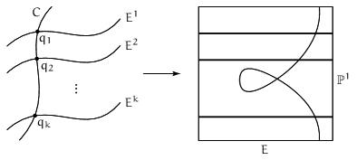
Figure 1. A curve with elliptic tails. We impose that each $E^{i}\to E\times{\mathbb{P}}^{1}$ is unramified.

The components of $\widetilde{V}^{\circ,\text{tails}}_{df+Ne,g}(\alpha,0)$ will be all equality cases. The result is the following.

Proposition 2.8.

Assume Hypothesis 1 and moreover that for generic $b\in V$, the map $C_{b}\to E\times{\mathbb{P}}^{1}$ has no floating components, and that the sections $\sigma_{i}(V)$ get contracted by the map $\varphi\colon{\mathcal{C}}\to E\times{\mathbb{P}}^{1}$ to points $p_{i}$, for all $i$. Then, $\dim V$ is at most $d+g-1$.

If equality occurs, then the image of $V$ in $|{\mathcal{L}}|$ is dense in a component of the Severi variety $\widetilde{V}^{\circ,\text{tails}}_{df+Ne,g}(\alpha,0)[p_{1},\ldots,p_{n}]$.

The following proof follows Proposition 3.4 in Vakil’s [Vak00] closely.

Proof.

After passing to a dominant generically finite cover of $V$, we may distinguish the components of $C_{b}$. If generically there are contracted components, discard them. This only makes the bound tighter.

Let us replace $C_{b}$ with its normalization $\widetilde{C_{b}}$. Again, this will only make the bound tighter. Let $k$ be the number of floating components in $\widetilde{C_{b}}$, and let $Y$ be the union of the other components. As the original curve $C_{b}$ did not have any floating component, there were at least $k$ nodes connecting them to other components of $\widetilde{C_{b}}$. Hence, the arithmetic genus of $p_{a}(Y)$ is at most $g-k$, with equality only if $C_{b}$ is equal to the curve $Y$ with $k$ elliptic tails attached.

Each floating component of $\widetilde{C_{b}}$ contributes to at most one dimension to $V$, because the map $V\to|{\mathcal{L}}|$ is generically finite, so the only moduli comes from picking the target fiber $E\times{\{{t}\}}$.

Let us focus on each component $X$ of $Y$ then. Let $\overline{X}$ be the image of $\varphi\colon X\to E\times{\mathbb{P}}^{1}$, and $\widetilde{X}\to\overline{X}$ its normalization. As $X$ is smooth, the map $X\to\overline{X}$ factors through $\widetilde{X}\to\overline{X}$. Moreover, since the fibers of $V\to|{\mathcal{L}}|$ are finite, a bound in the dimension in which $\widetilde{X}\to\overline{X}\subset E\times{\mathbb{P}}^{1}$ varies also bounds the dimension of $V$. Let $m$ be the degree of $X\to\widetilde{X}$. Summing over the components of $\widetilde{C_{b}}$, and applying Lemma 2.5, we get

$$\dim V \leq\left(\sum_{X\text{ floating}}\dim\left\{X\to E\times{\mathbb{P}}^{1}\right\}\right)+\left(\sum_{X\text{ not floating}}\dim\left\{\widetilde{X}\to E\times{\mathbb{P}}^{1}\right\}\right)$$

$$\leq\left(\sum_{X\text{ floating}}1\right)+\left(\sum_{X\text{ not floating}}\frac{d_{i}}{m}+p_{a}(\widetilde{X})-1\right)$$

$$\leq k+\left(\sum_{X\text{ not floating}}\frac{d_{i}}{m}+\frac{p_{a}(X)-1}{m}\right)$$

$$\leq k+\left(\sum_{X\text{ not floating}}d_{i}+p_{a}(X)-1\right)$$

$$=k+d+p_{a}(\widetilde{Y})-1$$

$$\leq k+d+(g-k)-1=d+g-1$$

as we wanted to show.

If equality holds, then $m=1$, $Y$ is a generic point of $V^{\circ}_{df+N^{\prime}e,g-k}(\alpha,0)$ and $C_{b}$ is a generic point in $\widetilde{V}^{\circ,\text{tails}}_{df+Ne,g}(\alpha,0)$. ∎

In our application, the intersection with $E_{0}$ will not be fixed. However, we can immediately adapt Proposition 2.8 to the following.

Corollary 2.9.

Assume Hypothesis 1 and that for generic $b\in V$, the map $C_{b}\to E\times{\mathbb{P}}^{1}$ has no floating components. There is a map $V\to E_{0}\times\ldots\times E_{0}$ that sends

$$b\mapsto\Bigl{(}\varphi(\sigma_{1}(b)),\ldots,\varphi(\sigma_{n}(b))\Bigr{)}$$

Let $P$ be the image of this map. Then

$$\dim V\leq d+g-1+\dim P$$

If equality holds, then each component of the fiber of $V\to P$ over $(p_{1},\ldots,p_{n})\in P$ is dense in a component of $\widetilde{V}^{\circ,\text{tails}}_{Ne+df,g}(\alpha,0)[p_{1},\ldots,p_{k}]$.

The elliptic tails arose naturally as an equality case in our dimension bound, but they do not actually occur as residual curves in the degeneration argument. To see that, we ask when elliptic tails can be smoothed away, that is, when is a map $f\colon C\to E\times{\mathbb{P}}^{1}$ with elliptic tails is a limit of a map with smooth source. By dimensional reasons, the general point of $V^{\circ,\text{tails}}_{df+Ne,g}\setminus V^{\circ}_{df+Ne,g}$ cannot be smoothed into $V^{\circ}_{df+Ne,g}$. But more is true—as long as $f$ is unramified, it cannot be smoothed!

Proposition 2.10.

Let $f\colon X=C\cup_{q}\widetilde{E}\to E\times{\mathbb{P}}^{1}$ be a finite flat unramified map from a nodal curve such that $\widetilde{E}$ lands in a $E$ fiber, and $\widetilde{E}\to E$ is an isogeny. Then the map $f$ cannot be deformed in a way that the node $q$ is smoothed.

In particular, no component of $V^{\circ,\text{tails}}_{Ne+df,g}(\alpha,0)$ is contained in the closure of $V^{\circ}_{df+Ne,g}$.

Proof.

By Theorem 5.1 of [Vis97], the deformations of the unramified map $f$ correspond to $\operatorname{Hom}_{{\mathcal{O}}_{X}}({\mathcal{N}}^{\vee}_{f},{\mathcal{O}}_{X})$, where ${\mathcal{N}}^{\vee}_{f}$ is the dual normal sheaf defined by:

(5) $$0\to{\mathcal{N}}^{\vee}_{f}\to f^{*}\Omega_{E\times{\mathbb{P}}^{1}}\to\Omega_{X}\to 0$$

The key computation is the following.

Claim 2.11.

The restriction ${\mathcal{N}}^{\vee}_{f}|_{\widetilde{E}}$ is equal to ${\mathcal{O}}_{\widetilde{E}}(-q)$.

This implies that the sheaf ${\mathcal{N}}^{\vee}_{f}$ is locally free at $q$. The map to the component of the $T^{1}_{X}$ sheaf supported on $q$ is just the restriction map

(6) $$\operatorname{Def}(f)=H^{0}(X,{\mathcal{N}}_{f})\to H^{0}(X,{\mathcal{N}}_{f}|_{q})=H^{0}(X,T^{1}_{X}|_{q})$$

To establish that the node $q$ cannot be smoothed away, we just need to show that the map in eq. 6 is zero. But the restriction map factors as

$$H^{0}(X,{\mathcal{N}}_{f})\to H^{0}(\widetilde{E},{\mathcal{N}}_{f}|_{\widetilde{E}})\to H^{0}(\widetilde{E},k_{q})$$

and the latter map $H^{0}(\widetilde{E},{\mathcal{N}}_{f}|_{\widetilde{E}})=H^{0}(\widetilde{E},{\mathcal{O}}_{\widetilde{E}}(q))\to H^{0}(\widetilde{E},k_{q})$ is zero, since

$$H^{0}(\widetilde{E},{\mathcal{O}}_{\widetilde{E}})\overset{\sim}{\to}H^{0}(\widetilde{E},{\mathcal{O}}_{\widetilde{E}}(q))\overset{0}{\to}H^{0}(\widetilde{E},k_{q})\overset{\sim}{\to}H^{1}(\widetilde{E},{\mathcal{O}}_{\widetilde{E}})$$

This finishes the proof of Proposition 2.10, given Claim 2.11. ∎

Proof of Claim 2.11.

Restricting the sequence (5), we get

(7) $$\operatorname{Tor}^{1}_{{\mathcal{O}}_{X}}(\Omega_{X},{\mathcal{O}}_{\widetilde{E}})\to{\mathcal{N}}^{\vee}_{f}|_{\widetilde{E}}\to\pi^{*}\Omega_{E\times{\mathbb{P}}^{1}}\to\Omega_{X}|_{\widetilde{E}}\to 0$$

where $\pi\colon\widetilde{E}\to E\times{\mathbb{P}}^{1}$ is the restriction of $f$ to $\widetilde{E}$. We can compute the extremal terms of the sequence as follows.

Claim 2.12.

The sheaf $\operatorname{Tor}^{1}_{{\mathcal{O}}_{X}}(\Omega_{X},{\mathcal{O}}_{\widetilde{E}})$ vanishes, and $\Omega_{X}|_{\widetilde{E}}=\Omega_{\widetilde{E}}\oplus k_{q}$.

Proof.

We only have to check this around the node $q$. We replace $X$ by $\operatorname{Spec}R$, for $R=k[x,y]/(xy)$, and $\widetilde{E}$ by the $x=0$ branch. Then $\Omega_{R}$ has the free resolution

$$0\to R\langle ydx+xdy\rangle\to R\langle dx,dy\rangle\to\Omega_{R}\to 0$$

Tensoring with $R/(x)$, we get the complex

$$0\to R/(x)\langle ydx\rangle\to R/(x)\langle dx,dy\rangle$$

This is exact at $R/(x)\langle ydx\rangle$, and hence $\operatorname{Tor}^{1}$ vanishes. The cokernel is $R/(x)\langle dy\rangle\oplus R/(x,y)\langle dx\rangle$, which implies that $\Omega_{X}|_{\widetilde{E}}=\Omega_{\widetilde{E}}\oplus k_{q}$. ∎

We use Claim 2.12 to simplify the sequence (7), and compare it to the normal sheaf sequence of $\pi\colon\widetilde{E}\to E\times{\mathbb{P}}^{1}$ as follows.

The snake lemma gives us the exact sequence

$$0\to{\mathcal{N}}^{\vee}_{f}|_{\widetilde{E}}\to{\mathcal{N}}^{\vee}_{\pi}\to k_{q}\to 0$$

Hence, it is enough to show that ${\mathcal{N}}^{\vee}_{\pi}={\mathcal{O}}_{\widetilde{E}}$. This in turn follows from the exact sequence

$$0\to{\mathcal{N}}_{\pi}^{\vee}\to\pi^{*}\Omega_{E\times{\mathbb{P}}^{1}}\to\Omega_{\widetilde{E}}\to 0$$

since $\pi^{*}\Omega_{E\times{\mathbb{P}}^{1}}=\Omega_{\widetilde{E}}\oplus{\mathcal{O}}_{\widetilde{E}}$, and the map to $\Omega_{\widetilde{E}}$ is the projection onto the first factor. ∎

2.1. Covers of $E$ of low gonality

In the proof of Lemma 2.5, we left two details to be checked later: that the general curve parametrized by $V_{df+Ne,g}(\alpha,0)$ does not have tacnodes, for $d=2$, and that it does not have triple points, for $d=3$. Fortunately, we can deal with these cases directly through ad hoc methods, as follows.

2.1.1. The hyperelliptic locus ($d=2$)

The intersection data with $E_{0}$ is an effective divisor $D=p_{1}+p_{2}$ on $E_{0}$, which is fixed. This defines a degree $2$ map $\varphi\colon E\to{\mathbb{P}}^{1}$. We will translate our problem of studying curves in $E\times{\mathbb{P}}^{1}$ to studying curves in ${\mathbb{P}}^{1}\times{\mathbb{P}}^{1}$, using the map

$$\Phi=(\varphi,id)\colon E\times{\mathbb{P}}^{1}\to{\mathbb{P}}^{1}\times{\mathbb{P}}^{1}$$

The divisor $D=p_{1}+p_{2}$ is a fiber of $\varphi$. Let $p_{0}=\Phi(p_{1})=\Phi(p_{2})$.

Let $C\subset E\times{\mathbb{P}}^{1}$ be a curve parametrized by $V_{df+Ne,g}(\alpha,0)[p_{1},p_{2}]$. Then the map $\Phi$ restricted to $C$ is two to one. Indeed, every intersection with $E\times{\{{t}\}}$ is linearly equivalent to $D$, and hence a fiber of $\varphi$.

Let $\overline{C}=\Phi(C)$ be its image. It has class $(N,1)$ in ${\mathbb{P}}^{1}\times{\mathbb{P}}^{1}$, and is a smooth rational curve. Note that $p_{0}\in\overline{C}$.

The map $\varphi\colon E\to{\mathbb{P}}^{1}$ has four branch points. Set

$$D={\{{\text{branch point of }f}\}}\times{\mathbb{P}}^{1}\subset{\mathbb{P}}^{1}\times{\mathbb{P}}^{1}$$

Away from $D$, the map $\Phi$ is étale. Hence, the curve $C$ can be singular only along the preimage of $D$. We can relate the singularity of $C$ with the tangency index of $\overline{C}$ with $D$. We exhibit the first cases in Table 1.

Singularity of $C$		Tangency of $\overline{C}$ with $D$
Type	Local Equation	Multiplicity	Local Equation
Smooth	$x=y^{2}$	$1$	$x=y$
Node	$x^{2}=y^{2}$	$2$	$x^{2}=y$
Cusp	$x^{3}=y^{2}$	$3$	$x^{3}=y$
Tacnode	$x^{4}=y^{2}$	$4$	$x^{4}=y$

Table 1. A dictionary between tangency conditions of $\overline{C}$ with $D$, and singularities of $C\subset E\times{\mathbb{P}}^{1}$.

We will constrain the tangency profile of $\overline{C}$ with $D$. Let

$$R =\sum_{p\in D}\left(\operatorname{mult}_{p}(\overline{C}\cdot D)-1\right)$$

$$=\overline{C}\cdot D-{|{\overline{C}\cap D}|}=4N-{|{\overline{C}\cap D}|}$$

This is the total ramification of $\overline{C}\to{\mathbb{P}}^{1}$ over the four branch points of $\varphi\colon E\to{\mathbb{P}}^{1}$. Let $E^{\times}$ (resp. $\left({\mathbb{P}}^{1}\right)^{\times}$) be the complement of the ramification (resp. branch) points of $\varphi$. Let $C^{\times}$ (resp. $\overline{C}^{\times}$) be the corresponding preimage. Using Riemann–Hurwitz, we can count the ramification as follows.

$$2g-2 =\operatorname{Ram}(\varphi\colon C\to E)$$

$$\geq\operatorname{Ram}(\varphi\colon C^{\times}\to E^{\times})$$

$$=2\operatorname{Ram}(\overline{C}^{\times}\to\left({\mathbb{P}}^{1}\right)^{\times})$$

$$=2\left(\operatorname{Ram}(\overline{C}\to{\mathbb{P}}^{1})-R\right)$$

$$=2(2N-2-R)=2({|{\overline{C}\cap D}|}-2N-2)$$

Equality holds only if $C\to E$ is not branched over the four ramification points of $\varphi$. However, if $\overline{C}$ had more than simple tangencies along $D$, then $C\to E$ would be ramified there, as we can see from the local equations in Table 1. Hence, if equalities hold, all tangencies of $\overline{C}$ with $D$ are simple, and the curve $C\subset E\times{\mathbb{P}}^{1}$ is nodal.

We can rewrite the inequality as

(8) $${|{\overline{C}\cap D}|}\leq 2N+g+1$$

We now invoke Theorem 2.1 to bound the dimension in which $\overline{C}\subset{\mathbb{P}}^{1}\times{\mathbb{P}}^{1}$ varies. Let $\Sigma$ be $\operatorname{Bl}_{p_{0}}{\mathbb{P}}^{1}\times{\mathbb{P}}^{1}$, the blow up of ${\mathbb{P}}^{1}\times{\mathbb{P}}^{1}$ at $p_{0}$, and set $\tau=Nf_{1}+f_{2}-e$, where $e$ is the exceptional divisor. We use the same $D$ as above, and set $\Omega=\varnothing$. By eq. 8, we may set $b=2N+g+1$. We have

$$\gamma =-(K_{\operatorname{Bl}_{p_{0}}{\mathbb{P}}^{1}\times{\mathbb{P}}^{1}}+D)\cdot\overline{C}+2N+g+1$$

$$=-(-2f_{1}+2f_{2}+e)(Nf_{1}+f_{2}-e)+2N+g+1$$

$$=-(2N-2+1)+2N+g+1=g+2$$

And hence the dimension bound

$$\dim V_{Ne+2f,g}(\alpha,0)\leq\gamma+0-1=g+1$$

On the other hand, by Lemma 2.4, the opposite inequality holds as well. Hence, all equalities hold, including in eq. 8. As $\gamma\geq 2$, Theorem 2.1 tell us that equality must hold in (8), and hence, $C$ is nodal, as we wanted to show.

2.1.2. The trigonal locus ($d=3$)

We now deal with the case of $V_{3f+Ne,g}(\alpha,0)$. We want to show that the general point corresponds to a nodal curve, and we just have to eliminate the case of triple points.

The tangency conditions with $E_{0}$ define a fixed divisor $D=p_{1}+p_{2}+p_{3}$ on $E_{0}$. This divisor defines an embedding of $E\hookrightarrow{\mathbb{P}}^{2}$ as a smooth cubic. Each intersection $C\cap\left(E\times{\{{t}\}}\right)$ maps to three collinear points in $E\subset{\mathbb{P}}^{2}$. We think of this as a map $\varphi\colon{\mathbb{P}}^{1}\to{\widehat{{\mathbb{P}}^{2}}}$ sending $t$ to the line joining the three collinear images of $C\cap\left(E\times{\{{t}\}}\right)$. Note that $\varphi(0)$ goes to the fixed line $\ell_{0}$ connecting the images of $p_{1},p_{2}$ and $p_{3}$.

Conversely, given the map $\varphi$, we can reconstruct $C$ as the intersection of $E\times{\mathbb{P}}^{1}\subset{\mathbb{P}}^{2}\times{\mathbb{P}}^{1}$ with the ruled surface in ${\mathbb{P}}^{2}\times{\mathbb{P}}^{1}$ traced out by the lines $\varphi(t)$ as we vary $t\in{\mathbb{P}}^{1}$. See fig. 2.

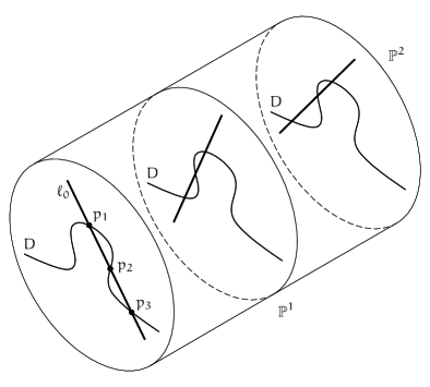
Figure 2. Recovering the curve $C$ as the intersection of $D\times{\mathbb{P}}^{1}$ and the ruled surface traced out by the lines $\varphi(t)$.

We can relate the singularities of $C$ with the tangency of the image of $\varphi$ along ${\widehat{E}}\subset{\widehat{{\mathbb{P}}^{2}}}$, the dual to $E\subset{\mathbb{P}}^{2}$. The dual ${\widehat{E}}$ is a degree $6$ curve with $9$ cusps (one for each flex of $E$).

If $C$ is singular at $(p,t)\in E\times{\mathbb{P}}^{1}$, then $\varphi(t)$ lies on ${\widehat{E}}$—specifically, at the point corresponding to the tangent to $E$ at $p$. Conversely, if we denote by $\widetilde{C}\to C$ the normalization map, we have:

• If $\varphi({\mathbb{P}}^{1})$ is transverse to ${\widehat{E}}$ at a point $\varphi(t)$, then $\widetilde{C}\to{\mathbb{P}}^{1}$ is simply branched over $t$, and $C$ is smooth at the corresponding point of $E\times{\mathbb{P}}^{1}$.

• If $\varphi({\mathbb{P}}^{1})$ is simply tangent to ${\widehat{E}}$ at a point $\varphi(t)$, then $C\subset E\times{\mathbb{P}}^{1}$ is nodal at the corresponding point, and $\widetilde{C}\to{\mathbb{P}}^{1}$ is not branched over $t$.

• If $\varphi({\mathbb{P}}^{1})$ does not contain any of the $9$ cusps of ${\widehat{E}}$, then $C$ has no triple points.

Hence, it is enough to show that the image of $\varphi({\mathbb{P}}^{1})$ has at most simple tangencies with ${\widehat{E}}$, and does not pass through any of the cusps. We will establish that by invoking once more Theorem 2.1, now to bound the dimension in which the image of $\varphi$ can vary.

By Riemann–Hurwitz, $\widetilde{C}\to{\mathbb{P}}^{1}$ has $2g+4$ branch points. Let $T$ be the number of transverse intersections of $\varphi({\mathbb{P}}^{1})$ and ${\widehat{E}}$. Hence $T\leq 2g+4$. Moreover,

$$6N =\varphi({\mathbb{P}}^{1})\cdot{\widehat{E}}$$

$$=\sum_{p}\operatorname{mult}_{p}(\varphi({\mathbb{P}}^{1})\cdot{\widehat{E}})$$

$$\geq T+2({|{\varphi({\mathbb{P}}^{1})\cap{\widehat{E}}}|}-T)$$

$$=2{|{\varphi({\mathbb{P}}^{1})\cap{\widehat{E}}}|}-T$$

$$\geq 2{|{\varphi({\mathbb{P}}^{1})\cap{\widehat{E}}}|}-(2g+4)$$

With equality holding only if at most simple tangencies occur. Rearranging, we get

(9) $$3N+g+2\geq{|{\varphi({\mathbb{P}}^{1})\cap{\widehat{E}}}|}$$

We set $\Sigma=\operatorname{Bl}_{\ell_{0}}{\widehat{{\mathbb{P}}^{2}}}$. The class $\tau$ of the proper transform of $\varphi({\mathbb{P}}^{1})$ is $Nh-e$, where $e$ is the class of the exceptional divisor. Using the notation of Theorem 2.1, and setting $b=3N+g+2$, we have

$$\gamma =-(K_{\Sigma}+{\widehat{E}})\cdot\tau+3N+g+2$$

$$=-(3h+e)(Nh-e)+3N+g+2$$

$$=-(3N+1)+3N+g+2=g+1$$

So the image of $\varphi({\mathbb{P}}^{1})$ can vary in at most $0-1+g+1=g$ dimensions. Adding $\dim(\operatorname{Aut}({\mathbb{P}}^{1},0))=2$ to remember the map $\varphi\colon{\mathbb{P}}^{1}\to{\widehat{{\mathbb{P}}^{1}}}$ (we know that $0$ maps to $\ell_{0}$), we get that the dimension of $V_{3f+Ne,g}(\alpha,0)$ is at most $g+2$. However, by Lemma 2.4, the opposite inequality holds as well. Hence, equality in (9) holds, and the original curve $C$ is nodal.

3. Hyperplane Sections of $\widetilde{V}^{\circ}_{Ne+df,g}(a,b)$

In this section, we will prove Theorems 1.18 and 1.20 stated in the introduction, and Theorem 3.13 which is a generalization of them. Let us briefly remind ourselves of the setup. We fix a fiber $E_{0}\subset E\times{\mathbb{P}}^{1}$, and let $p\in E_{0}$ be a general point. We want to characterize the irreducible components of of $\widetilde{V}^{\circ}_{Ne+df,g}(a,b)\cap H_{p}$. Let $W$ be one of these components, and $Y_{0}\subset E\times{\mathbb{P}}^{1}$ be the curve corresponding to a general point in $W$.

If the curve $Y_{0}$ does not contain $E_{0}$, it is easy to describe what $W$ must be—we will do that in Section 3.4. Let us assume, then, that the curve $E_{0}$ is contained in $Y_{0}$. Now it is much harder to analyze the residual curve. Our main tool to get our hands on its geometry is the following construction.

3.1. Nodal reduction

Pick a general point $Y_{0}\subset E\times{\mathbb{P}}^{1}$ in $W$. Choose a general arc $\Delta$ in $\widetilde{V}^{\circ}_{Ne+df,g}(a,b)$ approaching the point $(Y_{0})\in W$. We may assume that $\Delta$ is smooth by taking its normalization.

We get a flat family of curves mapping to $E\times{\mathbb{P}}^{1}$,

where the generic fiber is a general point in $\widetilde{V}^{\circ}_{Ne+df,g}(a,b)$, and the central fiber is a generic point in $W$. Let ${\mathcal{Y}}^{\times}$ be the restriction of ${\mathcal{Y}}$ over the punctured base $\Delta^{\times}$.

The preimage of $E_{0}\subset E\times{\mathbb{P}}^{1}$ under $\varphi$ on the punctured family ${\mathcal{Y}}^{\times}$ will consist of some multisections. After a a base change, we may assume that the multisections are actually sections. Being in $\widetilde{V}^{\circ}_{Ne+df,g}(a,b)$, there will be $a$ of those which get contracted under the map $\varphi$, and $b$ that are allowed to vary—that is, are not necessarily contracted by $\varphi$. To avoid overburden our notation even more, we will refer to these as $A$-sections and $B$-sections.

At this point there is not much we can say about the central fiber. However, if we perform nodal reduction on ${\mathcal{Y}}\to\Delta$, we can replace it by a more tractable object. Let us denote by ${\mathcal{C}}\to B$ the family obtained by nodal reduction, and $f\colon B\to\Delta$ the corresponding base change map. Here is what we can assume about it.

Hypothesis 2.

The family ${\mathcal{C}}\to B$ satisfies the following properties.

• The total space ${\mathcal{C}}$ is smooth.

• The fibers $C_{b}$ are equal to the corresponding fiber $Y_{f(b)}$ of the original family ${\mathcal{Y}}\to\Delta$, as long as $b\neq 0$.

• The (scheme-theoretic) central fiber $C_{0}$ is nodal (and therefore reduced).

• The maps $\varphi\colon C_{b}\to E\times{\mathbb{P}}^{1}$ are semistable.

• The preimage of $E_{0}$ is a union of sections of ${\mathcal{C}}\to B$, plus components in the central fiber. These sections are disjoint on the general fiber, but are allowed to meet along the central fiber. We will still call them A-sections and B-sections, as above.

• The family ${\mathcal{C}}\to B$ is the minimal one respecting the conditions above.

See fig. 3 for a diagram of the family ${\mathcal{C}}\to B$ away from the central fiber. Our goal is to determine how the central fiber looks like, and where the A and B-sections meet it.

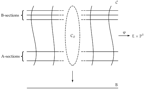
Figure 3. A diagram of the family ${\mathcal{C}}\to B$ away from the central fiber.

The idea of the proof of Theorem 1.18 is simple, but combinatorially challenging. There are two opposing forces controlling the central fiber. On one hand, it varies in a large dimension, and hence its singularities should be mild, and few extra conditions should be imposed. That is, the dimension count forces the central fiber to be “simple”. On the other hand, from the parametric point of view, the flatness of the family ${\mathcal{C}}$ says the central fiber has to have arithmetic genus $g$, and hence it cannot be too simple. We will determine the equilibrium positions, the conditions under which the two forces precisely cancel out. And it will turn out that these conditions completely describe the components of the hyperplane section.

To make the structure of the proof transparent, we will break up the argument into a chain of small claims. Each one will be an inequality expressing the tension between the two points of view. As we compose this long chain of inequalities, we will conclude that all equalities must hold! We then come back and use the equality conditions to pin down the possible components of the hyperplane section.

Again, we do not prove that all of these components do appear in a hyperplane section, or even if they do appear, we do not say with what multiplicity. Here we only compile a list of suspects: any component $W$ must be in this list.

The difficulty is that our starting point, the central fiber $C_{0}$, is an arbitrary nodal curve. Just notionally this is already very cumbersome. We have to design our notation to express all the arguments in this generality.

We divide the components of $C_{0}$ in three groups, forming nodal curves each:

• We call $\widetilde{E}$ the curve which is the union of irreducible components of $C_{0}$ that dominate $E_{0}$ under the map $\varphi\colon C_{0}\to E\times{\mathbb{P}}^{1}$.

• Let $Z$ be the union of the components that get contracted to a point in $E_{0}$ by the map $\varphi_{0}$.

• Let $X$ be the union of the remaining components.

Let $T$ be the number of connected components of $Z$ meeting both $X$ and $\widetilde{E}$, plus the number of nodes between $X$ and $\widetilde{E}$. For an example, see fig. 4.

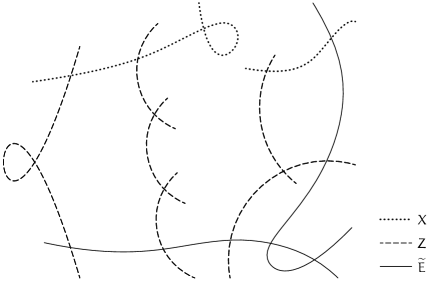
Figure 4. An example of an a priori possible central fiber $C_{0}$, with its components grouped as $\widetilde{E}$, $Z$ and $X$. In this example, $T=4$. The central fibers that do arise will turn out to be much simpler than this, as we will see.

3.2. The genus bound

In this section we will leverage the flatness of the family ${\mathcal{C}}\to B$ to bound the arithmetic genus of $X$ in terms of $g$ and $T$.

Start by enumerating the irreducible components of $Z$ by $Z_{1},\ldots,Z_{m}$. To help us keep track of the combinatorial data of $C_{0}$, we introduce an auxiliary graph $G$. We obtain $G$ by starting with the dual graph of the nodal curve $C_{0}$, and then collapsing the subgraph corresponding to components of $X$ (resp. $\widetilde{E}$) into a single vertex. Hence, it has $m+2$ vertices—one for each $Z_{i}$, and one for $\widetilde{E}$ and one for $X$, even though $\widetilde{E}$ and $X$ may well be reducible. The edges of $G$ correspond to the nodes of $C_{0}$ which are not internal to $X$ or $\widetilde{E}$—that is, we don’t consider nodes which connect two components of $X$, or two components of $\widetilde{E}$. In particular, there are no loops in $G$ at the vertices corresponding to $\widetilde{E}$ and $X$. We will refer to the nodes corresponding to edges in $G$ as external nodes. Note that the number of edges in $G$ is equal to the number of external nodes. For an example, see fig. 5.

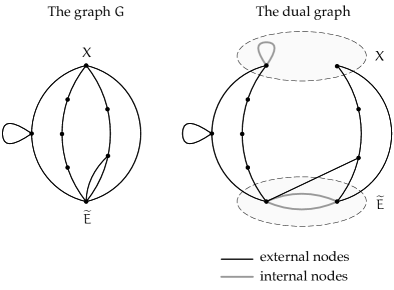
Figure 5. The dual graph of the example $C_{0}$ in fig. 4, and the respective graph $G$ obtained by contracting the subgraphs corresponding to $X$ and $\widetilde{E}$.

Claim 3.1.

Let $d_{X}$ (resp. $d_{\widetilde{E}}$) be the degree of $X$ (resp. $\widetilde{E}$) in the graph $G$. Then, $T\leq d_{X}$ and $T\leq d_{\widetilde{E}}$. If both equalities hold, then every connected component of $Z$ meets $X$ and $\widetilde{E}$ exactly once each.

Proof.

This follows directly from the definition of $T$. The inequality is strict in two situations: if there are connected components of $Z$ meeting only one of $X$ and $\widetilde{E}$, or if there are connected components of $Z$ meeting $X$ or $\widetilde{E}$ in more than one node. ∎

Claim 3.2.

Let $d_{Z_{i}}$ be the number of nodes on $Z_{i}$ in $C_{0}$, that is, the degree of $Z_{i}$ in the graph $G$. Then

$$0\leq g(Z_{i})-1+\frac{d_{Z_{i}}}{2}$$

with equality only if $Z_{i}$ is rational with exactly two nodes on it.

Proof.

This comes from the minimality of the family. If this quantity was negative, then $Z_{i}$ would be a rational curve meeting the rest of the central fiber at only one point. Then, we compute the intersection pairing on the surface ${\mathcal{C}}$:

$$0=Z_{i}C_{0}=Z_{i}^{2}+1$$

from which we conclude that $Z_{i}$ is a ($-1$)-curve. Moreover, being a component in $Z$, the map $\varphi$ contracts $Z_{i}$. Hence, we could contract it in ${\mathcal{C}}$ and maintain the conditions of Hypothesis 2, contradicting the minimality of ${\mathcal{C}}$.

If equality holds, then $g(Z_{i})=0$ and $d_{Z_{i}}=2$, as we want, or $g(Z_{i})=1$ and $d_{Z_{i}}=0$. The latter case does not occur, because $Z_{i}$ would be a disconnected component of $C_{0}$ which gets contracted under the map to $E\times{\mathbb{P}}^{1}$, and hence cannot be in the limit of maps $C_{t}\to E\times{\mathbb{P}}^{1}$ which are birational onto their image. ∎

Next, we compute the arithmetic genus of the central fiber. By summing the degrees of all vertices of $G$, we get twice the number of edges. That is,

$$d_{X}+d_{\widetilde{E}}+\sum d_{Z_{i}}=2\times{|{\text{edges in }G}|}=2\times{|{\text{ external nodes in }C_{0}}|}$$

Hence, we get

$$p_{a}(C_{0})-1 =p_{a}(X)-1+p_{a}(\widetilde{E})-1+\sum_{i=1}^{m}\left(g(Z_{i})-1\right)+{|{\text{external nodes in }C_{0}}|}$$

$$=p_{a}(X)-1+p_{a}(\widetilde{E})-1+\frac{d_{X}+d_{\widetilde{E}}}{2}+\sum_{i=1}^{m}\left(g(Z_{i})-1+\frac{d_{Z_{i}}}{2}\right)$$

Moreover, by flatness,

$$g-1=p_{a}(C_{t})-1=p_{a}(C_{0})-1$$

Summing up, we get the following.

Claim 3.3.

We have,

$$g-1=p_{a}(X)-1+p_{a}(\widetilde{E})-1+\frac{d_{\widetilde{E}}+d_{X}}{2}+\sum_{i=1}^{m}\left(g(Z_{i})-1+\frac{d_{Z_{i}}}{2}\right)$$

The last ingredient is the following.

Claim 3.4.

We have

$$0\leq p_{a}(\widetilde{E})-1$$

with equality only if $\widetilde{E}$ is a disjoint union of smooth genus 1 curves, and $\widetilde{E}\to E_{0}$ is unramified.

Proof.

This follows from the Riemann–Hurwitz formula applied to $\widetilde{E}\to E_{0}$. Note that $\widetilde{E}$ may be disconnected. ∎

We are ready for the following key bound.

Proposition 3.5.

[The Genus Bound] We have

$$p_{a}(X)+T\leq g$$

Equality holds only if $\widetilde{E}$ is smooth, $\widetilde{E}\to E$ is unramified, and $Z$ is a union of chains of rational curves connecting $X$ and $\widetilde{E}$.

The equality does not hold in our previous example fig. 4, but in fig. 6 we can see an example where it does hold.

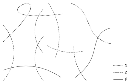
Figure 6. A picture of $C_{0}$ in a case where equality in the genus bound (Proposition 3.5) holds.

Proof.

Just add up the inequalities in Claims 3.1, 3.3, 3.2 and 3.4. If equality holds, then it does as well in every claim, and hence all equalities conditions are true.

From Claim 3.4 we get that $\widetilde{E}$ is smooth and $\widetilde{E}\to E$ is unramified. The equality conditions of Claim 3.2 imply that $Z$ is a disjoint union of chains of rational curves. Claim 3.1 implies that each of these chains connects a component of $\widetilde{E}$ to a component of $X$. ∎

Note that, so far, even if equality occurs in Proposition 3.5, we can’t say much about the residual curve $X$. Also note that we haven’t used the sections our family came equipped with either. These will play a role in the following.

3.3. The dimension bound

We now want to constraint the geometry of $X$ based on the fact it varies in a family of dimension $\dim W=\dim H_{p}\cap\widetilde{V}^{\circ}_{Ne+df,g}(a,b)=d+g+b-3$.

The construction in Section 3.1 replaces a general point $\{Y_{0}\subset E\times{\mathbb{P}}^{1}\}$ of the component $W$ with a map $C_{0}\to E\times{\mathbb{P}}^{1}$. To leverage the dimension of $W$, we need to extend this pointwise construction to a local one. The following technical lemma does so.

Lemma 3.6.

For each general point $p\in W$, we can find a map $\eta\colon U\to U_{0}\subset W$ which is finite onto a open subscheme which contains $p$, a flat family ${\mathcal{C}}^{U}\to U$ and a map $\varphi\colon{\mathcal{C}}^{U}\to E\times{\mathbb{P}}^{1}$ such that for each $u\in U$, the map $C^{U}_{u}\to E\times{\mathbb{P}}^{1}$ is equal to the result of the pointwise construction of Section 3.1 on $\eta(u)\in W$.

Proof.

The idea is the following: the only choice we had in the construction in Section 3.1 was of the arc $\Delta\to V$. However, as we are performing a codimension one degeneration, the limit will not depend on the direction of approach. Here is a standard way to formalize this.

The variety $\widetilde{V}^{\circ}_{Ne+df,g}(a,b)$ admits a rational map to the Kontsevich space of stable maps $\overline{M}_{g,a+b}(E\times{\mathbb{P}}^{1},df+Ne)$. Since the target is projective and the source is normal, we can extend the rational map in codimension one. Hence, for a general point in the divisor $H_{p}\cap\widetilde{V}^{\circ}_{Ne+df,g}(a,b)$, we can find a neighborhood of $p$ mapping to the coarse space $\overline{M}_{g,a+b}(E\times{\mathbb{P}}^{1},df+Ne)$. Possibly after a base change, we find some neighborhood $\widehat{U}$ which maps to the stack $\overline{{\mathcal{M}}}_{g,a+b}(E\times{\mathbb{P}}^{1},df+Ne)$. Now pulling back the universal family, we get a family ${\mathcal{C}}^{\widehat{U}}\to\widehat{U}$. Let $U\subset\widehat{U}$ be the preimage of $W$. Our universal family ${\mathcal{C}}^{U}\to U$ is the restriction of ${\mathcal{C}}^{\widehat{U}}\to\widehat{U}$. ∎

The total space ${\mathcal{C}}^{U}$ is reducible: there is at least a component containing the generic fiber’s $\widetilde{E}$, and a component containing the generic fiber’s $X$. We want to pick out the component ${\mathcal{X}}\subset{\mathcal{C}}^{U}$ corresponding to the $X$’s. A way to directly construct it is to set

$${\mathcal{X}}={\overline{{\mathcal{C}}-\varphi^{-1}(E_{0})}},\text{ where }\varphi\colon{\mathcal{C}}^{U}\to E\times{\mathbb{P}}^{1}$$

Let us denote the restriction of $\varphi\colon{\mathcal{C}}^{U}\to E\times{\mathbb{P}}^{1}$ to ${\mathcal{X}}$ by $\varphi$ again. We will bound arithmetic genus $p_{a}(X_{u})$ in terms of the dimension of $U$ and the tangency conditions the image of the $X_{u}$ satisfies along $E_{0}$, using Corollary 2.9.

To get our hands on the tangency conditions, we need to introduce some notation. Let $k$ be the cardinality of $\varphi^{-1}(E_{0})\cap X_{u}$ for $u$ generic. After a base change, we may assume that $\varphi^{-1}(E_{0})$ consists of $k$ distinct sections. Let $U\to E_{0}^{k}$ the map sending $u$ to the images under $\varphi$ of the $k$ sections. Let $P\subset E_{0}^{k}$ be the image of this map.

Each one of the $k$ sections appears with some multiplicity, say $\alpha_{i}$. We get a corresponding map

$$E_{0}^{k} \to\operatorname{Div}^{d}E_{0}$$

$$(p_{1},\ldots,p_{k}) \mapsto\sum\alpha_{i}p_{i}\in\operatorname{Div}^{d}E_{0}$$

For example, the composite map $U\to E_{0}^{k}\to\operatorname{Div}^{d}(E_{0})$ sends $u$ to the divisor $\varphi(X_{u})\cdot E_{0}$ on $E_{0}$.

Note that the linear class of $\varphi(X_{u})\subset E\times{\mathbb{P}}^{1}$ is equal to the class of $C_{0}$ minus some number of $E_{0}$’s that got split off. That is, $[\varphi(X_{u})]={\mathcal{L}}-me$, and the intersection $\varphi(X_{u})\cdot E_{0}={\mathcal{L}}|_{E_{0}}$ is a fixed linear class. Hence, the following diagram commutes.

Denote by $X$ the generic fiber $X_{u}$.

Claim 3.7.

We have

$$\dim W\leq d+p_{a}(X)-1+\dim P$$

If equality holds, then, after a base change, $W$ is fibered over $P$, and the the fiber over $(p_{1},\ldots,p_{k})\in P\subset E_{0}^{k}$ is dense in a component of

$$\widetilde{V}^{\circ,\text{tails}}_{df+N^{\prime}e,p_{a}(X)}(\alpha,0)[p_{1},\ldots,p_{k}]$$

where $\alpha_{i}$ is the multiplicity in which the section over the point $p_{i}$ appears, and $df+N^{\prime}e$ is the homology class of $\varphi(X)$.

Proof.

This follows from Corollary 2.9 applied to ${\mathcal{X}}\to U$, and the fact that $U$ and $W$ have the same dimension. ∎

To bound the dimension of $P$, let us go back to our one-dimensional degeneration ${\mathcal{C}}\to B$ as in Section 3.1. Let $\varepsilon_{b}$ be the number of B-sections which meet the central fiber on $\widetilde{E}$ or on a connected component of $Z$ that does not meet $X$. That is, out of the $b$ B-sections that the family ${\mathcal{C}}\to B$ has, $b-\varepsilon_{b}$ of them land in $X$, or in a component of $Z$ that contracts to a point in $X$. Either way, these $b-\varepsilon_{b}$ points are in the intersection of $\varphi(X)$ with $E_{0}$.

Define

$$\varepsilon=\begin{cases}1,\text{ if }\varepsilon_{b}>0\\ 0,\text{ else.}\end{cases}$$

For example, we have

(10) $$\varepsilon\leq\varepsilon_{b}$$

with equality only if $\varepsilon_{b}$ is equal to zero or one.

Now we are ready to state the bound on $\dim P$.

Claim 3.8.

We have

$$\dim P\leq T+b-\varepsilon_{b}-1-(1-\varepsilon)$$

If equality holds, none of the $A$ or $B$-sections land in components of $Z$ meeting $X$ and $\widetilde{E}$, and one of the two following scenarios holds.

1. If $\varepsilon=1$, then $P$ is dense in the preimage under $E_{0}^{k}\to\operatorname{Div}^{d}E_{0}$ of the sum of:

   • a full linear series of degree $T+b-\varepsilon_{b}$,

   • and $a^{\prime}=d-(T+b-\varepsilon_{b})$ base points.

2. Else, both $\varepsilon_{b}$ and $\varepsilon$ are zero, and $P$ is dense in the preimage under $E_{0}^{k}\to\operatorname{Div}^{d}E_{0}$ of the sum of:

   • a full linear series of degree $b$ on $E$ (corresponding to the limit of the B-sections),

   • a full linear series of degree $T$ on $E$,

   • and $a^{\prime}=d-b-T$ fixed base points.

Proof.

The curve $\varphi(X)$ meets $E_{0}$ in three types of points:

• The image of A-sections. These add no moduli to $P$.

• The images of B-sections. There are $b-\varepsilon_{b}$ of those.

• The images of connected components of $Z$ meeting both $X$ and $\widetilde{E}$, or nodes connecting $\widetilde{E}$ and $X$ in $C_{0}$. There are exactly $T$ of those.

Hence, the dimension of $P$ is bounded by

$$\dim P\leq T+b-\varepsilon_{b}$$

However, if equality were to hold, then $P$ would be dense in $E^{T+b-\varepsilon_{b}}\subset E^{k}$ for some subset of the indices. But $P\to E^{k}\to\operatorname{Div}^{d}E$ has to land inside the full linear series $\left|{\mathcal{L}}|_{E_{0}}\right|\subset\operatorname{Div}^{d}E$, while the image of $E^{T+b-\varepsilon_{b}}\subset E^{k}\to\operatorname{Div}^{d}E$ does not have a fixed linear class. This is a contradiction.

Hence, we get the slightly stronger inequality

$$\dim P\leq T+b-\varepsilon_{b}-1$$

for which equality happens exactly if $P$ is the preimage of some full linear series of degree $T+b-\varepsilon_{b}$, plus some fixed base points (which correspond to A-sections landing in $X$). That is, only in scenario (1).

Something interesting happens when $\varepsilon_{b}=0$. In this case, all the B-sections land in $X$, and their sum is a fixed divisor up to linear equivalence. Indeed, it is exactly the class of $\varphi(C_{t})={\mathcal{L}}$, restricted to $E_{0}$, minus the fixed images of the A-sections $p_{1},\ldots,p_{a}$. Hence, we get one moduli less than expected. That is, we may subtract $(1-\varepsilon)$ from the count above, to get to

$$\dim P\leq T+b-\varepsilon_{b}-1-(1-\varepsilon)$$

as we wanted to prove. Now equality happens in both scenarios (1) and (2). ∎

Putting all of this together, we get the following.

Proposition 3.9 (The dimension bound).

We have

$$g\leq p_{a}(X)+T$$

If equality holds, then there is a partition $\tau$ of length $T$, and an integer $a^{\prime}\leq a$, such that $X$ is a general point of

• $\widetilde{V}^{\circ,\text{tails}}_{df+N^{\prime}e,p_{a}(X)}(a^{\prime},b,\tau)$, if $\varepsilon=0$, or

• $\widetilde{V}^{\circ,\text{tails}}_{df+N^{\prime}e,p_{a}(X)}\left(a^{\prime},\tau+(b-1)\right)$, if $\varepsilon=1$.

Proof.

By Theorem 2.6, we have

$$\dim W=\dim\widetilde{V}^{\circ}_{Ne+df,g}(a,b)-1=d+g+b-3$$

Now combine Equation 10 and Claims 3.7 and 3.8, and we get the desired inequality.

If equality holds, we let $\tau=(\tau_{1},\tau_{2},\ldots)$, where $\tau_{i}$ is the multiplicity in which each of the corresponding $T$ points appear in the divisor $\varphi^{*}(E_{0})|_{X}$, and $a^{\prime}$ be the number of A-sections landing in $X$. Considering all the equality conditions together, we get the description above. ∎

3.4. Proof of Theorems 1.18 and 1.20

Let us start with Theorem 1.18. Let $W$ be an irreducible component of $\widetilde{V}^{\circ}_{Ne+df,g}(a,b)\cap H_{p}$. If the generic point of $W$ is a curve that does not contain $E_{0}$, then $W$ is contained in

$$\widetilde{V}^{\circ}_{Ne+df,g}(a+1,b-1)[p_{1},\ldots,p_{a},p]$$

However, by Theorem 2.6, this has the same dimension as $W$. Hence, $W$ must be one of its irreducible components, as we wanted to show.

Let us assume now that the general point of $W$ is a curve which contains $E_{0}$ with multiplicity $m>0$. Set $N^{\prime}=N-m$, so that the homology class of the residual curve, $\varphi(X)$, is $N^{\prime}e+df$.

Then we apply the results of Sections 3.3, 3.2 and 3.1. On one hand, Proposition 3.5 (the genus bound) says

$$p_{a}(X)+T\leq g$$

while Proposition 3.9 (the dimension bound) says

$$g\leq p_{a}(X)+T$$

Hence, both equalities have to hold! We can now use the equality conditions to describe the central fiber $C_{0}$ and the way the A and B-sections meet it.

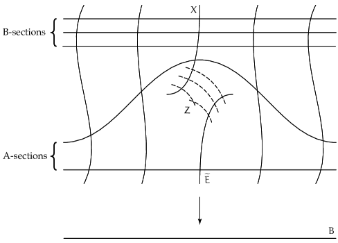
Figure 7. An example of a central fiber, and of the first of the two possible scenarios of how the sections meet the central fiber—never on the $Z$ components, and none of the B-sections meets $\widetilde{E}$.

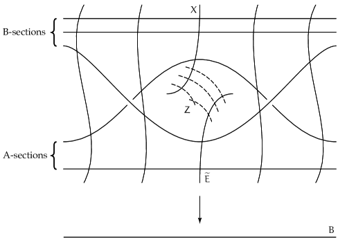
Figure 8. The same example of a central fiber as in fig. 7, but with the second possibility for how the sections meet the central fiber—again never on the $Z$ components, and with exactly one of the B-sections meeting $\widetilde{E}$.

By Proposition 3.5, the map $\widetilde{E}\to E$ is unramified, and $Z$ is just a disjoint union of $T^{\prime}$ rational chains connecting $X$ and $\widetilde{E}$, plus $(T-T^{\prime})$ nodes between $X$ and $\widetilde{E}$. Let $\tau$ be a partition keeping track of the multiplicities with which each of the $T$ rational chains/nodes connecting $X$ and $\widetilde{E}$ appears in the pullback $\varphi^{*}(E_{0})|_{X}$.

By Proposition 3.9, none of the A and B-sections hit the central fiber at $Z$. Let $a^{\prime}$ be the number of A-sections that land in $X$. In particular, $a^{\prime}\leq a$.

There are two possible scenarios for $X$, according to if there are any B-sections approaching $\widetilde{E}$ in the limit.

If there are B-sections approaching $\widetilde{E}$, then there is exactly one such. In this case, the residual curve $X$ is a general point of a component of the Severi variety $\widetilde{V}^{\circ,\text{tails}}_{N^{\prime}e+df,p_{a}(X)}\left(a^{\prime},\tau+(b-1)\right)$.

On the other hand, if there are no B-sections approaching $X$, then $X$ is a general point of a component of $\widetilde{V}^{\circ,\text{tails}}_{N^{\prime}e+df,p_{a}(X)}(a^{\prime},b,\tau)$. See figs. 7 and 8 for diagrams for the family ${\mathcal{C}}\to B$ and its sections.

There is one last issue to be taken care of: we have to eliminate the elliptic tails. This follows directly from Proposition 2.10. Note that this also rules out $\tau=(1)$—in this case, $\widetilde{E}$ itself would be an elliptic tail, which can’t be smoothed. This concludes the proof of Theorem 1.18.

Remark 3.10.

As opposed to the analogue arguments applied on rational surfaces [CH98, Vak00], our directrix $E_{0}$ can be split off generically with multiplicity greater than one. Compare with [SS13] where the “directrix” is still split off with multiplicity one, but the residual curve can be non-reduced.

To prove Theorem 1.20, we note that the nodal reduction construction in Section 3.1 already resolved the map $\widetilde{V}^{\circ}_{Ne+df,g}(a,b)\dasharrow\overline{{\mathcal{M}}}_{g}(E,N)$ at the general point of $W$. By composing the map $\varphi\colon C_{0}\to E\times{\mathbb{P}}^{1}$ with the projection $E\times{\mathbb{P}}^{1}\to E$, we get a map that is almost an element of $\overline{{\mathcal{M}}}_{g}(E,N)$—we just have to contract the rational chains $Z$. The description in Theorem 1.20 follows.

3.5. The general case

Let us tackle the problem of computing the degree of the Severi variety $V^{\circ}_{Ne+df,g}$. The strategy is to intersect it with multiple hyperplanes of the form $H_{p}$, for general $p\in E_{0}$, until we get down to some number of points, which we could count. Let $V$ be a component that arises in the process of intersecting $\widetilde{V}^{\circ}_{Ne+df,g}(a,b)$ with hyperplanes. To succeed, we have to answer the following two questions:

• what are the components of the intersection $V\cap H_{p}$?

• with what multiplicity does each component appear?

We will deal with only the first question. Theorem 1.18 describes the components of the intersections until the first time the directrix $E_{0}$ is split off generically. To continue, we would need an analogue of Theorem 1.18 for varieties like $\widetilde{V}^{\circ}_{N^{\prime}e+df,p_{a}(X)}(a^{\prime},b,\tau)$.

Fortunately, the argument above readily adapts to this more general situation, and all the components that ever arise in this process can be described in similar tangency terms. We will follow an analogue of Caporaso–Harris notation for these new components. The key difference in our case is that, since $E$ has non trivial Picard group, we are also forced to remember the classes of some of the moving points, as we already had in the case of $\widetilde{V}^{\circ}_{N^{\prime}e+df,p_{a}(X)}(a^{\prime},b,\tau)$.

Definition 3.11.

Fix line bundles ${\mathcal{L}},L_{j}\in\operatorname{Pic}E_{0}$, points $p_{1},\ldots,p_{k}\in E_{0}$, and tangency profiles $\alpha$ and $\beta^{1},\ldots,\beta^{\ell}$, such that $m(\beta^{j})=\deg L_{j}$ and

$${\mathcal{L}}=\sum_{i=1}^{k}\alpha_{i}p_{i}+\sum_{j=1}^{\ell}L_{j}$$

where $\alpha=(\alpha_{1}\ldots\alpha_{k})$. We define the generalized Severi variety

$$\widetilde{V}^{\circ}_{Ne+df,g}(\alpha,\beta^{1},\beta^{2},\ldots,\beta^{\ell})[p_{1},\ldots,p_{k},L_{1},\ldots,L_{\ell}]$$

as the normalization of the closure of the locus of reduced (possibly reducible) curves in $E\times{\mathbb{P}}^{1}$, of class $\pi_{1}^{*}{\mathcal{L}}\otimes\pi_{2}^{*}({\mathcal{O}}_{{\mathbb{P}}^{1}}(d))$, geometric genus $g$, containing no fibers of $E\times{\mathbb{P}}^{1}\to{\mathbb{P}}^{1}$, and whose intersection with $E_{0}$ consists of ${|{\alpha}|}+\sum_{j}{|{\beta^{j}}|}$ points as follows:

• The fixed points $p_{1},\ldots,p_{k}$, each appearing with the corresponding multiplicity $\alpha_{1},\ldots,\alpha_{k}$ (note that ${|{\alpha}|}=k$),

• and for each $j$, ${|{\beta^{j}}|}$ points with multiplicities described by $\beta^{j}$, and whose sum is linearly equivalent to $L_{j}$.

We will omit the brackets when possible, and just write $\widetilde{V}^{\circ}_{Ne+df,g}(\alpha,\beta^{1},\ldots,\beta^{\ell})$.

Note that by an argument similar to Theorem 2.6, we have

(11) $$\dim\widetilde{V}^{\circ}_{Ne+df,g}(\alpha,\beta^{1},\ldots,\beta^{\ell})=d+g+\sum_{j}{|{\beta^{j}}|}-1-\ell$$

and its generic point corresponds to a nodal curve.

Remark 3.12.

If for some $j$ we have $\beta^{j}=(b)$, then the generalized Severi variety is a disjoint union of $b^{2}$ different generalized Severi varieties, where we remove $\beta^{j}$ and add an extra $\alpha_{k+1}=b$, with the corresponding point $p_{k+1}$ being a $b$-th root of $L_{j}$. Hence, we may assume that ${|{\beta^{j}}|}\geq 2$ for all $j$.

We can now describe the components that will ever arise in the process of intersecting with the hyperplanes $H_{p}$’s.

Theorem 3.13.

Let $p$ be a generic point on $E_{0}$, and $W$ a component of the intersection $\widetilde{V}^{\circ}_{Ne+df,g}(\alpha,\beta^{1}\ldots,\beta^{\ell})\cap H_{p}$. Assume that $|\beta_{j}|\geq 2$ for all $j$. Then one of the following holds.

• Either $W$ is a component of

  $$\widetilde{V}^{\circ}_{Ne+df,g}(\alpha+(n),\beta^{1},\ldots,\beta^{j}-(n),\ldots,\beta^{\ell})[p_{1},\ldots,p_{k},p,L_{1},\ldots,L_{j}-p,\ldots L_{\ell}]$$

  for some $j$. That is, one of the moving points became a fixed at $p$.

• Or the elliptic fiber $E_{0}$ is generically split off in the limit with multiplicity $m$. As a parameter space for the residual curve, $W$ is a component of

  $$\widetilde{V}^{\circ}_{(N-m)e+df,g^{\prime}}(\alpha^{\prime},\beta^{j_{1}},\ldots,\beta^{j_{t}},\beta^{\prime})[p_{i_{1}},\ldots,p_{i_{{|{\alpha^{\prime}}|}}},L_{j_{1}},\ldots,L_{j_{t}},L^{\prime}]$$

  where

  1. $J={\{{j_{1},\ldots,j_{t}}\}}\subset[\ell]$ is a subset

  2. for $j\not\in J$, let $\widehat{\beta^{j}}\subset\beta^{j}$ be a tangency profile with one less term.

  3. $\tau$ is a tangency profile such that ${|{\tau}|}\geq 2$ and

     $$g=g^{\prime}+{|{\tau}|}$$

  4. $\beta$ is a tangency profile such that

     $$\beta^{\prime}=\tau+\sum_{j\not\in J}\widehat{\beta^{j}}$$

  5. and $\alpha^{\prime}\subset\alpha$ is a subprofile such that

     $$d=m(\alpha^{\prime})+m(\beta^{\prime})+\sum_{j\in J}m(\beta^{j})$$

  That is, for each group $\beta^{j}$ of B-sections, at most one of them may specialize to the curve dominating $E_{0}$. All the others stay in the residual curve. If the group of $\beta^{j}$ remains intact, then its class is preserved. Otherwise, all the $\beta^{j}$ that lost an element bundle up together, plus a partition $\tau$ that remembers how the residual curve meets the cover of $E_{0}$ in the stable limit.

Proof.

The argument will be very similar to the one for the simpler case of Theorem 1.18. As a matter of fact, the proof goes through mostly word by word—the only difference is that we have to do more bookkeeping to keep track of all the tangency profiles $\alpha,\beta^{j}$. Let us just highlight the differences, and leave the details to the reader.

Sections 3.1 and 3.2 go through as they are. In particular, we will use the same definition of $\widetilde{E},Z,X$ and $T$. We obtain Proposition 3.5 (the genus bound):

$$p_{a}(X)+T\leq g$$

In Section 3.3, the key adjustment is our definition of $\varepsilon_{b}$ and $\varepsilon$. We let $\varepsilon_{j}$ be the number of sections in the $\beta^{j}$ group which meet the central fiber on $\widetilde{E}$ or on a connected component of $Z$ that does not meet $X$. We define

$$\varepsilon={|{{\{{j\text{ such that }\varepsilon_{j}\neq 0}\}}}|}\\$$

From the definition of $\varepsilon$, we get the following.

Claim 3.14.

We have

$$\varepsilon\leq\sum_{j=0}^{\ell}\varepsilon_{j}$$

with equality only if, for each $j$, $\varepsilon_{j}$ is equal to zero or one.

And the corresponding Claim 3.8 is the following.

Claim 3.15.

We have

$$\dim P\leq T+\sum_{j}({|{\beta^{j}}|}-\varepsilon_{j})-(\ell-\varepsilon+1)$$

We get the dimension bound

$$g\leq p_{a}(X)+T$$

by coupling Claims 3.15, 3.14 and 3.7, and the following consequence of eq. 11:

$$\dim W=\dim V_{df+Ne,g}(\alpha,\beta)-1=d+g+(\sum|\beta^{j}|)-1-\ell-1$$

Again, the dimension bound balances exactly the genus bound, and equalities hold throughout. Analyzing the equality conditions, and eliminating elliptic tails by Proposition 2.10, we arrive at the list of Theorem 3.13. ∎

4. Monodromy Groups of Covers

In this section we will study the monodromy groups of simply branched covers.

Let $f\colon C\to D$ be a degree $d$ cover of smooth connected curves. Let $D^{\times}\subset D$ be the complement of the set of branch points of $f$, and $C^{\times}$ its preimage in $C$. We will deal with fundamental groups, so let us fix base points $\star\in D^{\times}$ and $\star\in C^{\times}$ that map to each other under $f$.

The map $f\colon C^{\times}\to D^{\times}$ is a covering of topological spaces. The fundamental group $\pi_{1}(D^{\times},\star)$ acts on the fiber $f^{-1}(\star)$. This action defines a monodromy map $\varphi\colon\pi_{1}(D^{\times},\star)\to S_{d}$. We call the image of $\varphi$ the monodromy group of the cover $f$. Note that it is only defined up to conjugation in $S_{d}$. If $\varphi$ is surjective, we say that $f$ has full monodromy.

A driving question in the field is what are the possible monodromy groups $G$. There are many interesting (and some unsolved) problems along this line, see for example, [Gur03, AP05, FM01, GMS03]. However, when the covering map $f$ is simply-branched, one can say much more.

Proposition 4.1 (Berstein–Edmonds).

Let $f\colon C\to D$ be a simply branched cover. Then $f$ has full monodromy if, and only if, $f$ is primitive (that is, the pushforward map in fundamental groups $\pi_{1}(C,\star)\to\pi_{1}(D,\star)$ is surjective).

This is Proposition 2.5 of [BE84]. One can find a proof of this in [Kan05b] as well. For completeness, here is a modified proof.

Proof.

From a factorization of $f\colon C\to D$ through a non-trivial unramified map $\widetilde{D}\to D$, we get a partition of $f^{-1}(\star)$ according to the different images in $\widetilde{D}$. The monodromy of $f$ has to preserve this partition, and hence cannot be the full symmetric group.

Suppose now that $f$ is primitive. We want to show it has full monodromy. Let $K$ be the kernel of the map $i_{*}\colon\pi_{1}(D^{\times},\star)\to\pi_{1}(D,\star)$. We start by showing the following.

Claim 4.2.

The action of $K$ on $f^{-1}(\star)$ is transitive.

Proof.

Consider the following commutative diagram of groups:

Given any element $g\in\pi_{1}(D^{\times},\star)$, we can use the surjectivity of the top and right arrows to find an element ${\overline{g}}\in\pi_{1}(C^{\times},\star)$ such that

$$i_{*}(g)=f_{*}i_{*}({\overline{g}})=i_{*}(f_{*}({\overline{g}}))$$

Hence,

$$g\cdot\left(f_{*}({\overline{g}})\right)^{-1}=\kappa\in K$$

Now let us consider the monodromy action of $g$ on the fiber $f^{-1}(\star)$. More specifically, let us see how $g$ acts on the base point $\star\in C^{\times}$ (which in turn lies over the base point $\star\in D^{\times}$).

If we lift a representative loop of $f_{*}({\overline{g}})$ with start point $\star$, we will get a representative loop of ${\overline{g}}$. Hence, the monodromy action of $f_{*}({\overline{g}})$ fixes $\star$. As $g=\kappa\cdot f_{*}({\overline{g}})$, we get $g(\star)=\kappa(\star)$.

We showed that for any $g\in\pi_{1}(D^{\times},\star)$, there is a $\kappa\in K$ that acts on $\star$ in the same way. Hence, the orbit of $\star$ under the $K$-action is equal to the orbit under the $\pi_{1}(D^{\times},\star)$-action. But the latter action is transitive, since $C^{\times}$ is connected. Hence, the action of $K$ is transitive as well. ∎

Claim 4.3.

The image of $K\subset\pi_{1}(D^{\times},\star)\to S_{d}$ is generated by transpositions.

Proof.

We use the standard presentations of $\pi_{1}(D,\star)$ and $\pi_{1}(D^{\times},\star)$. Let $g(D)$ be the genus of $D$. Then $\pi_{1}(D,\star)$ is the free group generated by $\alpha_{i},\beta_{i}$ for $i$ ranging from $1$ to $g(D)$, subject to the relation

$$[\alpha_{1},\beta_{1}]\ldots[\alpha_{g(D)},\beta_{g(D)}]=\operatorname{Id}$$

Let $b$ be the number of branch points of $f\colon C\to D$, and choose simple contractible loops $\tau_{j}$ around each branch point. Then $\pi_{1}(D^{\times},\star)$ is the free group generated by $\alpha_{i},\beta_{i}$ for $i=1,2,\ldots,g(D)$ and $\tau_{j}$ for $j=1,2,\ldots,b$, subject to the relation

$$[\alpha_{1},\beta_{1}]\ldots[\alpha_{g(D)},\beta_{g(D)}]=\tau_{1}\tau_{2}\ldots\tau_{b}$$

The map $\pi_{1}(D^{\times},\star)\to\pi_{1}(D,\star)$ sends the $\alpha_{i},\beta_{i}$ to the corresponding $\alpha_{i},\beta_{i}$, and each $\tau_{j}$ to $\operatorname{Id}$. Hence, the kernel $K$ is the normal closure of the subgroup generated by the $\tau_{j}$.

Since $f\colon C\to D$ is simply branched, each $\tau_{j}$ acts as a transposition. Hence so will any conjugate of $\tau_{j}$. Therefore, the image of $K$ in $S_{d}$ is generated by transpositions, as we wanted to show. ∎

Now we can finish the proof of Proposition 4.1. The image of $K$ in $S_{d}$ is transitive and generated by transpositions. But the only subgroup of $S_{d}$ satisfying these two properties is $S_{d}$ itself. Hence, $K\to S_{d}$ is surjective, and so is the monodromy map $\varphi\colon\pi_{1}(D^{\times},\star)\to S_{d}$. ∎

Corollary 4.4.

A primitive degree $d$ simply branched cover $f:C\to D$ does not admit any isomorphisms over $D$, unless $d=2$.

Proof.

This is similar to Proposition 1.9 in [Ful69]. An isomorphism of $C$ over $D$ corresponds to an element $\sigma$ of $S_{d}$ that commutes with every element of the monodromy group $\operatorname{im}\varphi\subset S_{d}$.

By Proposition 4.6, if a cover is primitive, then the monodromy map is surjective, and therefore $\sigma$ would be in the center of $S_{d}$, which is the trivial group as soon as $d\geq 3$. ∎

An arbitrary cover may be related to primitive ones by the following construction.

Corollary 4.5.

Let $f\colon C\to D$ be a simply branched covering map. Then it can be factored in a unique way as $C\to\overline{D}\to D$ such that $C\to\overline{D}$ has full monodromy, and $\overline{D}\to D$ is unramified.

Proof.

The unramified cover $\overline{D}\to D$ is the covering space corresponding to the subgroup $\operatorname{im}\pi_{1}(C,\star)\subset\pi_{1}(D,\star)$. By the lifting property, the map $C\to D$ factors through $\overline{D}$. The map $C\to\overline{D}$ is surjective on $\pi_{1}$. Hence, by Proposition 4.1, it has has full monodromy. ∎

Corollary 4.5 gives us a tool to study the monodromy group of an arbitrary simply branched cover $f\colon C\to D$. We would hope to relate the monodromy group of $f$ with the monodromy groups of each factor, which are easier to understand. The following proposition is a first step in this direction.

Proposition 4.6.

Let $C\to\overline{D}\to D$ be as in Corollary 4.5. Let $G$ (resp. $\overline{G}$) be the monodromy group of $C\to D$ (resp. $\overline{D}\to D$). The following holds.

1. There is a surjective map $G\twoheadrightarrow\overline{G}$,

2. There kernel of $G\twoheadrightarrow\overline{G}$ is as large as it can be. That is, the monodromy group $G$ fits in a exact sequence

   $$1\to S_{\widetilde{d}}\times\ldots\times S_{\widetilde{d}}\to G\to\overline{G}\to 1$$

   where the product in the left term has $\bar{d}=\deg(\overline{D}\to D)$ factors, each of them isomorphic to the symmetric group on $\widetilde{d}=\deg(C\to\overline{D})$ elements.

Proof.

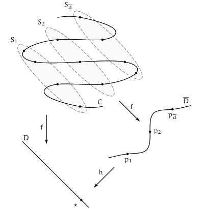
Figure 9. The preimages of $\star$ in $\overline{D}$ and $C$.

We will define a map $G\to\overline{G}$ such that the monodromy maps are compatible. That is, we want the following diagram to commute

The map is defined as follows. Given a monodromy element $g\in G$, choose a representative loop $\gamma\colon I\to D^{\times}$ inducing it. We send $g$ to $\overline{g}=\overline{\varphi}(i_{*}(\gamma))$. Geometrically, $\overline{g}$ is the monodromy element induced by the intermediate lifts of $\gamma$ to $\overline{D}$:

The map $G\to\overline{G}$ is well defined because if a loop $[\gamma]\in\pi_{1}(D^{\times},\star)$ induces the trivial monodromy on the fibers of $C\to D$, it also induces the trivial monodromy on the fibers of the intermediate map $\overline{D}\to D$.

Since $i_{*}\colon\pi_{1}(D^{\times},\star)\to\pi_{1}(D,\star)$ and $\overline{\varphi}\colon\pi_{1}(D,\star)\to\overline{G}$ are surjective, so is the map $G\to\overline{G}$. This establishes item 1.

Let us introduce some notation. Let $\overline{f}\colon C\to\overline{D}$ and $h\colon\overline{D}\to D$ be the factors of the factorization of $f\colon C\to D$. Call $p_{1},\ldots,p_{\bar{d}}\in\overline{D}$ the points in the preimage of $\star\in D$, and let $S_{i}=\overline{f}^{-1}(p_{i})\subset C$. See fig. 9.

Let $K$ be the kernel of $G\twoheadrightarrow\overline{G}$. The elements of $K$ preserve the sets $S_{i}$ for all $i$. That is, $K\subset\operatorname{Sym}(S_{1})\times\operatorname{Sym}(S_{2})\times\ldots\times\operatorname{Sym}(S_{\bar{d}})\subset\operatorname{Sym}(\cup S_{i})$. We want to show that $K=\operatorname{Sym}(S_{1})\times\operatorname{Sym}(S_{2})\times\ldots\times\operatorname{Sym}(S_{\bar{d}})$.

Pick a simple loop $\gamma\in\pi_{1}(D^{\times},\star)$, contractible in $D$, around one of the branch points. Let $\tau=\varphi(\gamma)\in G$ be the corresponding monodromy element. It is a transposition, since the branching is simple. Moreover, since $\gamma$ is contractible in $D$, the transposition $\tau$ maps to the identity in $\overline{G}$. Hence $\tau\in K$. The transposition $\tau$ has to act trivially in all but one of the $S_{i}$. Say it acts non-trivially on $S_{1}$. By a slight abuse of notation, we will say that $\tau\in\operatorname{Sym}(S_{1})$.

We will exploit the action of $G$ on $K$ by conjugation. First, consider the composition of the pushforward $h_{*}:\pi_{1}(\overline{D}^{\times},p_{1})\to\pi_{1}(D^{\times},\star)$ with the monodromy map $\varphi_{f}:\pi_{1}(D^{\times},\star)\to G$. The composite map $\varphi_{f}\circ h_{*}$ fixes $S_{1}$, and hence it factors through $\operatorname{Sym}(S_{1})\times\operatorname{Sym}(S_{2}\cup\ldots\cup S_{\bar{d}})$. Projecting on the $\operatorname{Sym}(S_{1})$ factor, we recover the monodromy map of $C\to\overline{D}$, as in the following diagram.

Pick $\gamma\in\pi_{1}(\overline{D}^{\times},p_{1})$. Conjugating an element of $\operatorname{Sym}(S_{1})\cap K$ by $\varphi_{f}(h_{*}(\gamma))$ is the same as conjugating by $\varphi_{\overline{f}}(\gamma)\in\operatorname{Sym}(S_{1})$. As $C\to\overline{D}$ has full monodromy, we can get an arbitrary conjugate in $\operatorname{Sym}(S_{1})$.

We already have a transposition $\tau\in\operatorname{Sym}(S_{1})\cap K$. Hence, we can get all transpositions in $\operatorname{Sym}(S_{1})$. But these generate the full symmetric group. Hence, $\operatorname{Sym}(S_{1})\times\operatorname{Id}\times\operatorname{Id}\times\ldots\times\operatorname{Id}\subset K$.

For each $i$, pick $\overline{g}\in\overline{G}$ that sends $p_{1}$ to $p_{i}$. Lift $\overline{g}$ to $g\in G$. Then

$$g\operatorname{Sym}(S_{1})g^{-1}=\operatorname{Sym}(S_{i})\subset K$$

As this holds for any $i$, we get

$$\operatorname{Sym}(S_{1})\times\operatorname{Sym}(S_{2})\times\ldots\times\operatorname{Sym}(S_{\bar{d}})\subset K$$

as we wanted to show. ∎

Note that the exact sequence in Proposition 4.6 does not completely characterize the monodromy group $G$—we do not know what extension it is. Determining what extensions do arise as monodromy groups of simply branched maps is an interesting question, which, as far as I know, is unsolved.

We now apply Proposition 4.6 to establish the result we will need in Section 5.

Lemma 4.7.

Let $C$ be a smooth curve, $C\to\overline{D}$ be a simply branched map with full monodromy, and $\overline{D}\to D$ an unramified map. Consider the map

$$C\times_{D}C-\Delta\to\overline{D}\times_{D}\overline{D}$$

The target $\overline{D}\times_{D}\overline{D}$ is smooth, but possibly disconnected. Nevertheless, the preimage of each component is irreducible.

Proof.

Let $\Gamma\subset\overline{D}\times_{D}\overline{D}$ be a component. We want to show that its preimage is connected.

If $\Gamma=\Delta$ is the diagonal, having connected preimage is equivalent to the monodromy group of $C\to\overline{D}$ being 2-transitive. This is immediate, since the monodromy group is actually the full symmetric group.

Suppose now $\Gamma$ is not the diagonal. For convenience, let us use the notation as in the proof of Proposition 4.1. Pick a point in the fiber over $\star$ of the map $\Gamma\to D$, say $(p_{i},p_{j})$. For any $q_{i},q^{\prime}_{i}\in S_{i}$ and $q_{j},q_{j}^{\prime}\in S_{j}$, we want to exhibit a path in $C\times_{D}C$ connecting $(q_{i},q_{j})$ to $(q^{\prime}_{i},q^{\prime}_{j})$. It is enough to find an element in the monodromy group of $C\to D$ that sends $q_{i}$ to $q^{\prime}_{i}$, and $q_{j}$ to $q^{\prime}_{j}$. This follows from Proposition 4.1, since the monodromy group contains $\operatorname{Sym}(S_{i})\times\operatorname{Sym}(S_{j})$. ∎

5. Irreducibility of the Hurwitz Space ${\mathcal{H}}^{0}_{N,g}(E)$

Let us resume our study of Hurwitz spaces. Recall their definition.

Definition 5.1.

The Hurwitz space ${\mathcal{H}}_{N,g}(E)$ parametrizes simply branched covers (meaning, dominant finite flat morphisms) $C\to E$ from a smooth genus $g$ curve $C$ to the fixed curve $E$. The space ${\mathcal{H}}^{0}_{N,g}(E)$ is the open and closed subscheme of ${\mathcal{H}}_{N,g}(E)$ of primitive covers $C\to E$ (that is, covers which do not factor through any non-trivial unramified maps $\widetilde{E}\to E$).

There are several alternate characterizations of ${\mathcal{H}}^{0}_{N,g}(E)$. For example, as a consequence of Proposition 4.1 and Corollary 4.5, we have the following useful one.

Proposition 5.2.

The space ${\mathcal{H}}^{0}_{N,g}(E)\subset{\mathcal{H}}_{N,g}(E)$ consists of the covers $C\to E$ with full monodromy.

Our goal is to prove Theorem 1.4, which says that for a smooth genus one curve $E$ and $g>1$, the Hurwitz space ${\mathcal{H}}^{0}_{N,g}(E)$ is irreducible. Note that from the irreducibility of ${\mathcal{H}}^{0}_{N,g}(E)$, we can characterize all the irreducible components of ${\mathcal{H}}_{N,g}(E)$.

Corollary 5.3.

The components of ${\mathcal{H}}_{N,g}(E)$ are in bijection with isogenies $\widetilde{E}\to E$ of degree diving $N$. That is, the decomposition in irreducible components is

$${\mathcal{H}}_{N,g}(E)=\bigsqcup_{\widetilde{E}\to E}{\mathcal{H}}_{N^{\prime},g}^{0}(\widetilde{E})$$

where $N^{\prime}=N/\deg(\widetilde{E}\to E)$, for $N^{\prime}\geq 2$.

Proof.

The right hand side is included in the left by the map

$$(C\to\widetilde{E})\mapsto(C\to\widetilde{E}\to E)$$

Corollary 4.5 says that the opposite inclusion holds, and Theorem 1.4 says every term in the right is irreducible. ∎

5.1. Our strategy

As a motivating example, let us go over a simple argument by Fulton for the irreducibility of ${\mathcal{M}}_{g}$ (in the appendix of [HM82]). We follow Harris and Morisson account in [HM98].

The idea, which really goes back to Deligne and Mumford, is to look instead at the compactified $\overline{{\mathcal{M}}_{g}}$ and leverage the structure of the boundary to prove irreducibility. More precisely, assume by induction that ${\mathcal{M}}_{g^{\prime}}$ is irreducible for $g^{\prime}<g$. Then, by induction, one can establish that each boundary divisor $\Delta_{i}$ in $\overline{{\mathcal{M}}_{g}}$ is irreducible. Moreover, one can prove that any pair of boundary divisors meet, simply by exhibiting an element in the intersection $\Delta_{i}\cap\Delta_{j}$. Hence, there is a unique connected component of $\overline{{\mathcal{M}}_{g}}$ meeting the boundary $\Delta$.

However, $\overline{{\mathcal{M}}_{g}}$ is locally irreducible, and therefore connectedness implies irreducibility. Hence, we established the following reduction.

Reduction.

It is enough to show that every component $\Gamma$ of $\overline{{\mathcal{M}}_{g}}$ meets the boundary $\Delta$.

To exhibit such a curve, we will pass to a more structured space: the Hurwitz space ${\mathcal{H}}_{d,g}({\mathbb{P}}^{1})$ of degree $d$ covers $C\to{\mathbb{P}}^{1}$. It follows from Riemann–Roch that for large $d$ the Hurwitz space dominates ${\mathcal{M}}_{g}$.

If we were willing to use that the Hurwitz space is irreducible, we would conclude irreducibility of ${\mathcal{M}}_{g}$ as well. However, using the reduction above, we can still prove irreducibility of $\overline{{\mathcal{M}}_{g}}$ without invoking the irreducibility of ${\mathcal{H}}_{d,g}({\mathbb{P}}^{1})$. Instead, we will use the properness of the admissible covers compactification $\overline{{\mathcal{H}}_{d,g}}({\mathbb{P}}^{1})$.

The branch morphism extends to the boundary of the admissible covers compactification, and every component of $\overline{{\mathcal{H}}_{d,g}}({\mathbb{P}}^{1})$ dominates the Fulton–MacPherson configuration space ${\mathbb{P}}^{1}[b]$. By choosing an extremal configuration of branch points, we can force the cover to be a reducible curve whose all irreducible components are rational. In particular, it is an element of $\Delta$. For details, see [HM98, Chapter 6A].

We will apply a similar argument to show the irreducibility of ${\mathcal{H}}_{N,g}^{0}(E)$. Again, the thrust of the argument comes from exploiting boundary divisors in a compactification of ${\mathcal{H}}_{N,g}^{0}(E)$. So let us start by choosing one.

A natural candidate is to use the Kontsevich space $\overline{{\mathcal{M}}}_{g}(E,N)$. However, this can have bad singularities at the locus of stable maps with contracted components, and it is not clear that it is locally irreducible, which is key to an argument like the one above.

We will instead use a partial compactification which is smooth, but still allows enough singular covers $X\to E$ for our reduction argument to go through.

Definition 5.4.

Let $\widetilde{{\mathcal{H}}}_{N,g}(E)\subset\overline{{\mathcal{M}}}_{g}(E,N)$ to be the open substack parametrizing finite maps (that is, the complement of the locus where there are contracted components). Points in $\widetilde{{\mathcal{H}}}_{N,g}(E)$ correspond to degree $N$, dominant, finite flat maps from a connected, arithmetic genus $g$ nodal curve $X$ to $E$. There is an open and closed substack $\widetilde{{\mathcal{H}}}^{0}_{N,g}(E)\subset\widetilde{{\mathcal{H}}}_{N,g}(E)$ parametrizing primitive covers.

Remark 5.5.

Not being primitive is naturally a closed property, since if a family of covers $X_{t}\to E$ factors through $\widetilde{E}\to E$ for generic $t$, then it factors through for all $t$. This implies that $\widetilde{{\mathcal{H}}}^{0}_{N,g}(E)\subset\widetilde{{\mathcal{H}}}_{N,g}(E)$ is an open substack.

However, it is also closed. Indeed, say $\widetilde{E}\to E$ is a non-trivial isogeny, and the composition $X_{0}\to\widetilde{E}\to E$ is a stable map which is a limit of primitive maps $X_{t}\to E$. Then $(X_{0}\to E)$ is a singular point of $\overline{{\mathcal{M}}}_{g}(E,N)$. Indeed, it lies in at least two components: the closure of ${\mathcal{H}}^{0}_{N,g}(E)$, and the closure of ${\mathcal{H}}^{0}_{N^{\prime},g}(\widetilde{E})$, where $N^{\prime}$ is the degree of $X_{0}\to\widetilde{E}$. Both of these components are already $2g-2$ dimensional, so $(X_{0}\to E)$ is a singular point. But, as we will see below in Lemma 5.6, ${\widetilde{{\mathcal{H}}}_{N,g}(E)}$ lives in the smooth locus of $\overline{{\mathcal{M}}}_{g}(E,N)$, so we would not see such a $X_{0}\to E$.

Lemma 5.6.

The space $\widetilde{{\mathcal{H}}}_{N,g}(E)$ is non-singular.

Proof.

The tangent space at a point $f:C\to E$ is equal to $H^{0}(C,{\mathcal{N}}_{f})$, where the normal sheaf ${\mathcal{N}}_{f}$ is defined as

$$0\to T_{C}\to f^{*}T_{E}\to{\mathcal{N}}_{f}\to 0$$

When there are no contracted components, ${\mathcal{N}}_{f}$ is torsion. Hence, $H^{1}(C,{\mathcal{N}}_{f})=0$, and Riemann–Roch says $h^{0}(C,{\mathcal{N}}_{f})=2g-2$, the length of the branch subscheme. As $\dim\widetilde{{\mathcal{H}}}_{N,g}(E)$ is $2g-2$ as well, we conclude it is non-singular. ∎

We will show that $\widetilde{{\mathcal{H}}}_{N,g}^{0}(E)$ is connected. Of course, Theorem 1.4 follows from this. Our proof will be inductive.

Induction Hypothesis 1.

Suppose, by induction, that the Hurwitz space of primitive covers $\widetilde{{\mathcal{H}}}_{N,g^{\prime}}^{0}(E)$ is connected for all genus one curves $E$, and integers $N\geq 2$ and $2\leq g^{\prime}<g$.

The base case $g=2$ is due to Kani in [Kan03].

Theorem (Kani).

The Hurwitz space ${\mathcal{H}}^{0}_{N,2}(E)$ is irreducible.

We will assume $g\geq 3$ from now on.

As in Fulton’s argument, let us take advantage of the boundary in our partial compactification. Call $\Delta\subset\widetilde{{\mathcal{H}}}_{N,g}^{0}(E)$ the locus of covers with singular source.

As opposed to the case of $\overline{{\mathcal{M}}_{g}}$, where there are relatively few boundary divisors and they are easily understood by induction, our boundary $\Delta$ will have quite a few boundary components, and they are not so easily dealt with inductively. Nevertheless, we will prove the following.

Final Reduction 1.

It is enough to show that every connected component of $\widetilde{{\mathcal{H}}}_{N,g}^{0}(E)$ contains a point in the boundary $\Delta$. That is, it is enough to find, in each component, a cover with singular source.

In Section 5.2 we will prove Final Reduction 1 under the Induction Hypothesis 1. Then in Section 5.3 we will establish that every component of Hurwitz space does contain a point of $\Delta$. As in Fulton’s argument, we have to pass to a more structured space to find such a point. In our case, we will use the Severi variety of curves in $E\times{\mathbb{P}}^{1}$. Specifically, we will invoke Theorem 1.20.

5.2. The reduction argument

In this section we will prove Final Reduction 1 under the Induction Hypothesis 1. To do so, we will first focus on a few special boundary divisors, and then bootstrap to the whole boundary $\Delta$.

We define $D_{\text{sing}}\subset\widetilde{{\mathcal{H}}}_{N,g}^{0}(E)$ to be the closure of the locus of covers $X\to E$ with $X$ irreducible and with a single node, for which the composition of the normalization map $\widetilde{X}\to X$ and $X\to E$ is primitive. That is, $\widetilde{X}\to E$ does not factor through non-trivial isogenies, as in the diagram in fig. 10.

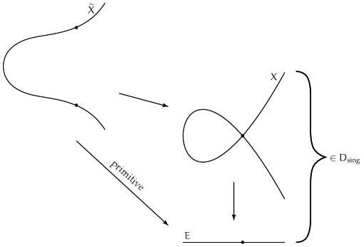
Figure 10. General point of $D_{\text{sing}}$

Lemma 5.7.

Under Induction Hypothesis 1, the set $D_{\text{sing}}$ is an irreducible divisor.

Proof.

We may parametrize the points in $D_{\text{sing}}$ by the data of a primitive cover $\pi\colon C\to E$ in ${\mathcal{H}}^{0}_{d,g-1}(E)$, and a pair of distinct points $p,q\in C$ in a fiber of $\pi$. This data is recorded in the fiber product $\Sigma={\mathcal{C}}\times_{E}{\mathcal{C}}-\Delta$, where ${\mathcal{C}}$ is the universal curve over ${\mathcal{H}}_{N,g-1}^{0}(E)$, and $\Delta$ is the diagonal. There is a birational isomorphism from $\Sigma$ to $D_{\text{sing}}$ that identifies the points $p$ and $q$. Note that

$$\dim D_{\text{sing}}=\dim\Sigma=2(g-1)-2+1=2g-3=\dim{\mathcal{H}}^{0}_{d,g}(E)-1$$

Hence $D_{\text{sing}}$ is a divisor. Moreover, from the induction hypothesis, we know that ${\mathcal{H}}_{N,g-1}^{0}(E)$ is irreducible. From Proposition 5.2, the monodromy of $C\to E$ is full, and therefore 2-transitive. Hence, $\Sigma$ is irreducible, and so is $D_{\text{sing}}$. ∎

From the Lemma 5.7, we get our first reduction.

Reduction 1.

It is enough to show that every connected component of $\widetilde{{\mathcal{H}}}^{0}_{N,g}(E)$ contains a point in $D_{\text{sing}}$.

Proof.

By Lemma 5.6, $\widetilde{{\mathcal{H}}}_{N,g}^{0}(E)$ is smooth, and hence it is enough to show it is connected. However, by Lemma 5.7, only one connected component meets $D_{\text{sing}}$. ∎

Let us define a few more special boundary divisors. For each isogeny ${\pi\colon\widetilde{E}\to E}$, let $D_{\pi}\subset\widetilde{{\mathcal{H}}}_{N,g}^{0}(E)$ be the closure of the subscheme parametrizing covers with reducible source $X=X^{\prime}\cup_{p}\widetilde{E}$, with a single node $p$, such that $X^{\prime}\to E$ is a primitive cover of degree $N-\deg\pi$, and genus $g-1$. See fig. 11 for a picture of the general point of $D_{\pi}$.

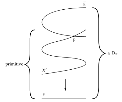
Figure 11. General point of $D_{\pi}$

Remark 5.8.

Given two pointed covers $f_{i}\colon(C_{i},p_{i})\to E$, for $i=1,2$, we can form a cover $f\colon C\to E$ by attaching $C_{2}$ to $C_{1}$ in the following way. Take

$$C=C_{1}\sqcup C_{2}/(p_{1}\sim p_{2})$$

and glue $f_{1}$ to $\tau\circ f_{2}$ where $\tau\colon E\to E$ is the translation which takes $f_{2}(p_{2})$ to $f_{1}(p_{1})$.

We may omit the point $p_{i}\in C$ in case $C_{i}\to E$ is an isogeny, since then the choice of point is irrelevant.

For example, a cover in $D_{\pi}$ is obtained by attaching the isogeny $\pi$ to a cover $X^{\prime}\to E$ in ${\mathcal{H}}^{0}_{N-\deg\pi,g-1}(E)$.

Lemma 5.9.

Under Induction Hypothesis 1, the set $D_{\pi}$ is an irreducible divisor.

Proof.

There is a map from the universal curve ${\mathcal{C}}\to\widetilde{{\mathcal{H}}}^{0}_{N-\deg\pi,g-1}(E)$ to $D_{\pi}$, which takes a pointed cover $(X^{\prime},p)\to E$ and attaches the isogeny $\pi\colon\widetilde{E}\to E$ at the marked point $p$. We conclude that $D_{\pi}$ is a divisor, since

$$\dim D_{\pi}=\dim{\mathcal{C}} =\dim{\mathcal{H}}^{0}_{N-\deg\pi,g-1}+1$$

$$=2(g-1)-2+1=2g-3=\dim{\mathcal{H}}^{0}_{N,g}(E)-1$$

Moreover, by induction, the universal curve ${\mathcal{C}}$ is irreducible, and so is $D_{\pi}$. ∎

We are on our way to prove

Reduction 2.

It is enough to show that every connected component of $\widetilde{{\mathcal{H}}}_{N,g}^{0}(E)$ contains a point in $D_{\text{sing}}$ or in $D_{\pi}$ for some isogeny $\pi$.

Indeed, this follows will follow from the Reduction 1 and the following proposition.

Proposition 5.10.

The union

$$D_{\text{sing}}\cup\bigcup_{\pi}D_{\pi}\subset\widetilde{{\mathcal{H}}}_{N,g}^{0}(E)$$

is connected, where $\pi$ ranges through all isogenies $\pi:\widetilde{E}\to E$ of degree at most $N-1$.

In view of irreducibility of $D_{\pi}$ and $D_{\text{sing}}$, it is enough to prove that these divisors meet for every $\pi$. That is, we only have to exhibit a curve that is in both.

Here is a candidate. Let $d$ be the degree of the isogeny $\pi\colon\widetilde{E}\to E$. Take a cover $\widetilde{X}_{0}\to E$ in ${\mathcal{H}}_{N-d,g-2}(E)$. Now pick two points $p_{1},p_{2}\in\widetilde{X}_{0}$ in a fiber of the map to $E$, and glue them to get a nodal curve $X_{0}\to E$. Then, pick a generic third point $q\in X_{0}$, and attach a copy of $\widetilde{E}$ at $q$. Let this be $X\to E$, as in fig. 12.

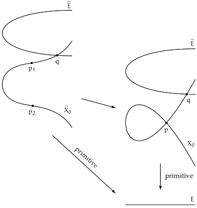
Figure 12. A cover in both $D_{\pi}$ and $D_{\text{sing}}$

From the definitions of $D_{\pi}$ and $D_{\text{sing}}$, we make the following observation.

Observation 5.11.

If $\widetilde{X}_{0}\cup\widetilde{E}\to E$ and $X\to E$ are both primitive covers, then $X\to E$ is a cover in the intersection $D_{\text{sing}}\cap D_{\pi}$.

Corollary 5.12.

If $g\geq 4$, then $D_{\text{sing}}$ meets $D_{\pi}$ for every isogeny $\pi$.

Proof.

When $g-2\geq 2$, we may choose a primitive cover $\widetilde{X}_{0}\to E$. This guarantees that both conditions in Observation 5.11 are satisfied. ∎

This settles Proposition 5.10 for $g\geq 4$, and in consequence the Reduction 2.

We can apply the same construction for $g=3$, but then $\widetilde{X}_{0}\to E$ would be an isogeny. We have to choose it carefully so that the hypotheses of Observation 5.11 are satisfied. It turns out that we cannot choose such a $\widetilde{X}_{0}\to E$ for every isogeny $\pi$, but we can for a large subclass: the reduced ones.

Definition 5.13.

An isogeny $\pi\colon\widetilde{E}\to E$ is reduced if it does not factor through the multiplication by $n$ map $M_{n}\colon E\to E$ for any integer $n>1$.

Lemma 5.14.

For any reduced isogeny $\pi\colon\widetilde{E}\to E$ and any $D\geq 2$, there is a reduced degree $D$ isogeny $\widehat{\pi}\colon\widehat{E}\to E$ and points $p_{1},p_{2}\in\widehat{E}$ such that

1. There is no common non-trivial subcover to $\pi$ and $\widehat{\pi}$.

2. For any subcover $\pi^{\prime}\colon\widehat{E}\to E^{\prime}$, the points $\pi^{\prime}(p_{1}),\pi^{\prime}(p_{2})\in E^{\prime}$ are the same if and only if $\pi^{\prime}=\widehat{\pi}$ (that is, the subcover is trivial).

We will prove Lemma 5.14 in Section 5.4.

Corollary 5.15.

For $g=3$ and a reduced isogeny $\pi$, the divisor $D_{\pi}$ meets $D_{\text{sing}}$.

Proof.

Take $\widetilde{X}_{0}$ as the $\widehat{E}$ produced by Lemma 5.14. This satisfies the conditions of Observation 5.11. ∎

To finish the proof of Proposition 5.10, for each isogeny $\pi$, we need to find a reduced isogeny $\pi^{\prime}$ such that $D_{\pi}$ meets $D_{\pi^{\prime}}$.

Lemma 5.16.

For $g=3$, the divisors $D_{\pi_{1}}$ and $D_{\pi_{2}}$ meet if $d_{1}+d_{2}=N-1$, where $d_{i}$ is the degree of the isogeny $\pi_{i}\colon\widetilde{E}_{i}\to E$.

Proof.

Form the nodal curve $X$ with components $\widetilde{E}_{1},\widetilde{E}_{2}$ and $E$, by gluing $\widetilde{E}_{1}$ with $E$ at a point $p$, and $\widetilde{E}_{2}$ with $E$ at a point $q\neq p$, as in fig. 13. The cover $X\to E$ lies in both $D_{\pi_{1}}$ and $D_{\pi_{2}}$.

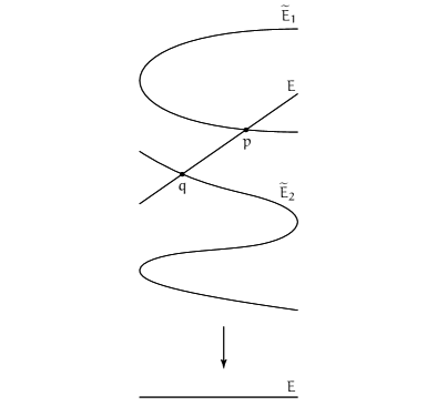
Figure 13. A cover in both $D_{\pi_{1}}$ and $D_{\pi_{2}}$.

∎

This completes the proof of Proposition 5.10, since there are reduced isogenies of any degree. This is easy to see directly, but is already a consequence of Lemma 5.14, so we are not going to restate it as a separate claim.

We have so far settled Reduction 2. This gives a good mileage towards our goal, the Final Reduction 1. To help organize what is left to do, let us introduce a piece of language.

Definition 5.17.

Let $C\to E$ be a cover in $\widetilde{{\mathcal{H}}}^{0}_{N,g}(E)$, and $\eta\in C$ a node in the source. Let $\widetilde{C}$ be the partial normalization of $C$ at $\eta$. We call $\eta$

• a disconnecting node if $\widetilde{C}$ is disconnected.

• a $E$-superfluous node if $\widetilde{C}$ is connected and $\widetilde{C}\to E$ is primitive.

• a $E$-relevant node if $\widetilde{C}\to E$ is not primitive, i.e., it factors through a non-trivial isogeny.

In this language, a cover is in $D_{\text{sing}}$ if and only if it has an $E$-superfluous node. We can reexpress Reduction 2 as saying that it is enough to find, in each connected component, a cover with an $E$-superfluous node, or a disconnecting node such that if the two components of the partial normalization are $C_{1}\sqcup C_{2}$, then

1. $C_{1}\to E$ is an isogeny, and

2. $C_{2}\to E$ is primitive.

We can relax this and drop condition (1).

Reduction 3.

It is enough to find, in each connected component of Hurwitz space ${\mathcal{H}}^{0}_{N,g}(E)$, a cover $C\to E$ with an $E$-superfluous node or a disconnecting node such that the restriction of $C_{1}\sqcup C_{2}\to C\to E$ to $C_{2}\to E$ is primitive.

Proof.

Indeed, let us say we have a cover $C\to E$ and a disconnecting node $\eta\in C$ such that such that $C_{2}\to E$ is primitive. If $C_{1}\to E$ is an isogeny, this is a point in $D_{\pi}$, and we are done. Assume otherwise that $C_{1}\to E$ is not an isogeny. We want to find another point in the same connected component which is in one of the $D_{\pi}$ divisors.

Let $\pi\colon\widetilde{E}\to E$ the maximal isogeny for which $C_{1}\to E$ factors through, and let $\eta_{1}\in C_{1}$ be the point over the node $\eta$. Then $(C_{1},\eta_{1})\to\widetilde{E}$ is an element of ${\mathcal{C}}\to\widetilde{{\mathcal{H}}}^{0}_{N_{1},g_{1}}(\widetilde{E})$, the universal curve over the component of Hurwitz space $C_{1}\to E$ lies on. By the Induction Hypothesis 1, ${\mathcal{C}}$ is irreducible. Hence, we can connect $(C_{1},\eta_{1})$ to any other element of ${\mathcal{C}}$. For example, we can take $(C^{\prime}\cup_{p}\widetilde{E},\eta^{\prime})\to\widetilde{E}$, where $\eta^{\prime}\in C^{\prime}$, for some cover $C^{\prime}\to\widetilde{E}$.

Attaching $(C_{2},\eta)\to E$ back to $(C^{\prime}\cup\widetilde{E},\eta^{\prime})\to\widetilde{E}\to E$, we get

$$X=\widetilde{E}\cup_{p}C^{\prime}\cup_{\eta}C_{2}\to E$$

as in fig. 14. As $C_{2}\to E$ is primitive, so is $C^{\prime}\cup_{\eta}C_{2}\to E$. Hence, the cover $X\to E$ is an element of $D_{\pi}$.

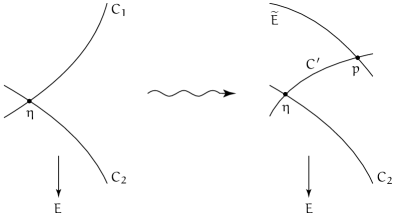
Figure 14. From a disconnecting node with a primitive component to a cover in $D_{\pi}$, as in Reduction 3.

∎

Remark 5.18.

Note that for this argument it was important that our induction hypothesis accommodates for any genus one target, as long as the genus of the source is smaller than $g$.

We can do even better.

Reduction 4.

It is enough to find, in each connected component of Hurwitz space, a cover with an $E$-superfluous node or a disconnecting node.

Proof.

We use the same trick. Let $C_{1}\sqcup C_{2}\to C\to E$ be the partial normalization of a curve with a disconnecting node $\eta$. Let $\eta_{i}\in C_{i}$ be the point over $\eta$. As $g\geq 3$, at least one of the $C_{i}$ has genus at least $2$. Say that is $C_{1}$. Let $\widetilde{E}\to E$ be the maximal isogeny $C_{1}\to E$ factors through. Degenerate $(C_{1},\eta_{1})\to E$ to $(C^{\prime}\cup\widetilde{E},\widetilde{\eta})\to E$ with $\widetilde{\eta}\in\widetilde{E}$. Attaching $(C_{2},\eta_{2})$ back, we get $C^{\prime}\cup_{p}\widetilde{E}\cup_{\eta}C_{2}\to E$, as in fig. 15.

Figure 15. From a cover with a disconnecting node to a cover with a disconnecting node and a primitive component, as in Reduction 4.

We claim that cover $\widetilde{E}\cup_{\eta}C_{2}\to E$ is primitive. Suppose not. Then, by definition, the map ${\widetilde{E}\cup_{\eta}C_{2}\to E}$ factors through a non-trivial isogeny, and so would the original cover ${C_{1}\cup_{\eta}C_{2}\to E}$ (because $C_{1}\to E$ itself factors through $\widetilde{E}\to E$). But the original cover is primitive by assumption, which is a contradiction.

Hence, the node $p$ joining $C^{\prime}$ and $\widetilde{E}$ is a disconnecting node for which one of the components is primitive. So we are done by Reduction 3. ∎

Let us finally prove the Final Reduction 1.

Proof.

Let $C\to E$ be a cover in $\Delta\subset\widetilde{{\mathcal{H}}}^{0}_{N,g}(E)$. Hence, $C$ has a node, call it $\eta$. By Reduction 4, it is enough to show that in the connected component of $C\to E$ there is a cover with an $E$-superfluous or a disconnecting node.

If $\eta$ itself is $E$-superfluous or disconnecting, we are done. We may assume that $\eta$ is $E$-relevant, then. This means that the partial normalization $\widetilde{C}\to E$ is connected, and that it factors through a non-trivial isogeny $\widetilde{E}\to E$. Let $\eta_{1},\eta_{2}\in\widetilde{C}$ be the preimages of the node $\eta$, and $N^{\prime}=\deg(\widetilde{C}\to\widetilde{E})$, as in fig. 16.

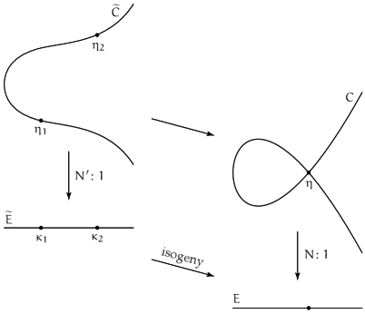
Figure 16. An $E$-relevant node $\eta$.

The data of $C\to E$ is encoded in the cover $\widetilde{C}\to\widetilde{E}$, with the two marked points $\eta_{1},\eta_{2}$. Let us construct a parameter space ${\mathcal{P}}$ for the triples $(\widetilde{C}\to\widetilde{E},\eta_{1},\eta_{2})$.

Let ${\mathcal{C}}\to\widetilde{{\mathcal{H}}}^{0}_{N^{\prime},g-1}(\widetilde{E})$ be the universal curve over the component of Hurwitz parametrizing primitive covers. The individual covers $C_{b}\to\widetilde{E}$ assemble together in a map ${\mathcal{C}}\to\widetilde{E}$. Then the triple $(\widetilde{C}\to\widetilde{E},\eta_{1},\eta_{2})$ is a point in

$${\mathcal{P}}={\mathcal{C}}\times_{E\times\widetilde{{\mathcal{H}}}}{\mathcal{C}}-\Delta$$

where the map from ${\mathcal{C}}$ to $E$ is the composition of ${\mathcal{C}}\to\widetilde{E}$ with the isogeny $\widetilde{E}\to E$.

Conversely, given any point $(\widetilde{C}^{\prime}\to\widetilde{E},\widetilde{\eta}_{1},\widetilde{\eta}_{2})\in{\mathcal{P}}$, we may identify the points $\widetilde{\eta}_{1}$ and $\widetilde{\eta}_{2}$ to get a cover $C^{\prime}\to E$ in $\widetilde{{\mathcal{H}}}^{0}_{N,g}(E)$.

This prompt us to characterize the connected component of ${\mathcal{P}}$ containing the point ${(\widetilde{C}\to\widetilde{E},\eta_{1},\eta_{2})}$. If this connected component contains a point which gives rise to a cover of $E$ with a disconnecting or $E$-superfluous node, we will be done.

Let $\kappa_{i}$ be the image of $\eta_{i}$ in $\widetilde{E}$. If $\kappa_{1}=\kappa_{2}$, then $C\to E$ would also factor through $\widetilde{E}\to E$, which is contrary to our assumption that $C\to E$ is primitive. Hence ${\kappa_{1}\neq\kappa_{2}}$. We can even say more: after identifying $\kappa_{1}$ with $\kappa_{2}$, the map from the nodal curve $\widetilde{E}/(\kappa_{1}\sim\kappa_{2})$ to $E$ is a primitive cover.

Note that the evaluation map ${\mathcal{C}}\to\widetilde{E}$ produces a map

$$f\colon{\mathcal{P}}={\mathcal{C}}\times_{E\times\widetilde{{\mathcal{H}}}}{\mathcal{C}}-\Delta\to\widetilde{E}\times_{E}\widetilde{E}$$

Our point $(\widetilde{C}\to\widetilde{E},\eta_{1},\eta_{2})$ in ${\mathcal{P}}$ maps to $(\kappa_{1},\kappa_{2})$.

We describe the components of ${\mathcal{P}}$ in terms of the map $f$.

Proposition 5.19.

The map $f\colon{\mathcal{P}}\to\widetilde{E}\times_{E}\widetilde{E}$ induces a bijection in connected components.

Before we prove this proposition, let us see how to establish the Final Reduction 1 assuming it.

If $g\geq 4$, we will use the construction in Figure 17. Take a primitive cover $C_{0}\to\widetilde{E}$ in ${\mathcal{H}}^{0}_{N^{\prime},g-2}(\widetilde{E})$. Pick a pair of distinct points $p_{1},p_{2}\in C_{0}$ in a generic fiber of the map to $\widetilde{E}$. Identify $p_{1},p_{2}$ to get a cover $C_{1}\to\widetilde{E}$ with a node $p$. Note that the node $p$ is $\widetilde{E}$-superfluous, by construction.

Pick any preimages $\eta^{\prime}_{i}\in C_{1}$ of $\kappa_{i}\in\widetilde{E}$. By Proposition 5.19, ${(C_{1}\to\widetilde{E},\eta_{1}^{\prime},\eta_{2}^{\prime})}$ is in the same component of ${\mathcal{P}}$ as the original $(\widetilde{C}\to E,\eta_{1},\eta_{2})$. Hence, if we identify $\eta^{\prime}_{1}$ with $\eta^{\prime}_{2}$, we get a primitive cover $C_{2}\to E$ in the same component as the original cover $C\to E$. However, $C_{2}\to E$ has two nodes: $\eta^{\prime}$ and $p$. But as $p$ was $\widetilde{E}$-superfluous, it is $E$-superfluous as well. By Reduction 4, we are done.

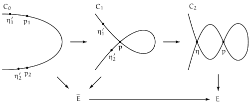
Figure 17. The construction for the case $g\geq 4$.

If $g=3$, we have to use a different argument, because there are no primitive genus 2 covers of $\widetilde{E}$ with an $\widetilde{E}$-superfluous node. Nevertheless, we can take an isogeny $\widetilde{E}_{0}\to\widetilde{E}$ of degree $N^{\prime}-1$, and attach an $\widetilde{E}$ tail. Let the resulting cover be $C_{0}=\widetilde{E}_{0}\cup_{p}\widetilde{E}\to\widetilde{E}$, as in Figure 18.

Now take $\kappa_{1},\kappa_{2}\in\widetilde{E}\subset C_{0}$. By Proposition 5.19, $(C_{0},\kappa_{1},\kappa_{2})$ is in the same connected component as $(\widetilde{C},\eta_{1},\eta_{2})$. Let $C_{1}$ be the nodal curve obtained by identifying $\kappa_{1}$ and $\kappa_{2}$ in $C_{0}$. We can degenerate our original cover $C\to E$ into $C_{1}\to E$. But $p\in C_{1}$ is a disconnecting node! Hence, by Reduction 4, we are done.

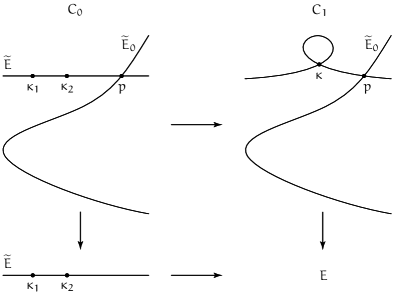
Figure 18. The construction for the case $g=3$.

∎

Proof of Proposition 5.19.

Recall that $\widetilde{E}\to E$ is an isogeny, and ${\mathcal{C}}\to\widetilde{{\mathcal{H}}}^{0}_{N^{\prime},g-1}(\widetilde{E})$ is the universal curve. The space ${\mathcal{P}}={\mathcal{C}}\times_{E}{\mathcal{C}}-\Delta$ parametrizes covers $C\to\widetilde{E}$ and pairs of distinct points $p_{1},p_{2}\in C$ that map to the same point $q\in E$ under the composite map $C\to\widetilde{E}\to E$. Hence, there is a map ${\mathcal{P}}\to E\times\widetilde{{\mathcal{H}}}^{0}_{N^{\prime},g-1}(\widetilde{E})$ which sends $(C\to\widetilde{E},p_{1},p_{2})$ to $(C\to\widetilde{E},q)$. This turns ${\mathcal{P}}$ into a finite cover of an irreducible target. Hence ${\mathcal{P}}$ is equidimensional, i.e., all components of ${\mathcal{P}}$ have the same dimension.

Now fix a component $\Gamma\subset\widetilde{E}\times_{E}\widetilde{E}$, and let

$${\mathcal{P}}_{\Gamma}=f^{-1}(\Gamma)\subset{\mathcal{P}}$$

where $f$ is the map $f\colon{\mathcal{P}}\to\widetilde{E}\times_{E}\widetilde{E}$. We want to show that ${\mathcal{P}}_{\Gamma}$ is irreducible. There is a forgetful map

$$\pi\colon{\mathcal{P}}_{\Gamma}\to\widetilde{{\mathcal{H}}}^{0}_{N^{\prime},g-1}(\widetilde{E})$$

sending $(C\to\widetilde{E},p_{1},p_{2})$ to $(C\to\widetilde{E})$. The fiber of $\pi$ over $C\to\widetilde{E}$ is

$$\pi^{-1}((\varphi\colon C\to\widetilde{E}))={\{{p_{1},p_{2}\in C,(\varphi(p_{1}),\varphi(p_{2}))\in\Gamma\text{ and }p_{1}\neq p_{2}}\}}$$

which is the same as saying that the fiber of $\pi$ is the preimage of $\Gamma$ in the map ${C\times_{E}C-\Delta\to\widetilde{E}\times\widetilde{E}}$. Hence, the following diagram is Cartesian.

Now observe that

• the target of $\pi$ is irreducible, by Induction Hypothesis 1,

• all fibers of $\pi$ have dimension one,

• the general fiber of $\pi$ is irreducible: more precisely, if $C\to\widetilde{E}$ is simply branched, then Lemma 4.7 says that the fiber of $\pi$ is irreducible.

Moreover, we already know that ${\mathcal{P}}_{\Gamma}$ is equidimensional. Hence, it follows that ${\mathcal{P}}_{\Gamma}$ is irreducible. ∎

5.3. The degeneration argument

Given Final Reduction 1, to complete the proof of Theorem 1.4 it is enough to prove the following.

Proposition 5.20.

Every component of $\widetilde{{\mathcal{H}}}_{N,g}^{0}(E)$ meets the boundary $\Delta$.

We will use our study of hyperplane sections of $\widetilde{V}_{df+Ne,g}(E)$ to produce such a cover in $\Delta$.

Proof.

Choose $d$ large enough so that the Severi variety $\widetilde{V}_{df+Ne,g}(E)$ dominates the Hurwitz space $\widetilde{{\mathcal{H}}}_{N,g}(E)$. For example, by Riemann–Roch $d=g+3$ is enough. For any component of $\widetilde{{\mathcal{H}}}_{N,g}^{0}(E)$, there is a component of $\widetilde{V}_{df+Ne,g}(E)$, say $V_{0}$, dominating it. Now intersect $V_{0}$ with multiple hyperplanes of the form $H_{p}$, as in Section 3. Eventually the curve $E_{0}\subset E\times{\mathbb{P}}^{1}$ is split off generically. We want to see what the image of this generic point is in the Hurwitz space $\widetilde{{\mathcal{H}}}_{N,g}^{0}(E)\subset\overline{{\mathcal{M}}}_{g}(E,N)$. The map is initially not defined there, but Theorem 1.20 tells us how to extend it. The resulting cover has singular source and there are no contracted components. Hence it is a point of $\Delta\subset\widetilde{{\mathcal{H}}}_{N,g}^{0}(E)$. ∎

This finishes the proof of Theorem 1.4.

Let us mention two alternatives ways to establish Proposition 5.20 in a more topological vein. To produce a node in the source, we have to bring a pair branch points together, in a way that, just before they meet, their monodromy transpositions exchange the same pair of sheets. To ensure this, we have to choose the path of approach carefully.

If one keeps track of how the permutation data changes as the branch points move around, one can re-encode the question in a combinatorial setting—we want to show that from any initial data, there is a sequence of moves that will result in a pair of adjacent branch points with the same monodromy transposition. However, it is still a tough problem. For example, in [GHS02, Kan05b], they can exhibit such a sequence of moves only when there are at least $2d-2$ branch points.

In [BE84], Berstein and Edmonds ask the same combinatorial problem, but allowing not only the moves on the branch points, but also Dehn twists on the target. In Proposition 5.2 of [BE84], they show that under this setup, whenever the target has genus one, we can apply a sequence of moves to produce a pair of adjacent branch points with the same monodromy. Tracing back through their argument, we see that no Dehn twists are used, so their result holds in our setup as well, effectively proving Proposition 5.20.

As the genus of the target increases, the combinatorial problem gets even harder. Gabai and Kazez get around this challenge with the following beautiful construction.

Lemma 5.21 (Gabai–Kazez).

For an arbitrary smooth curve $D$, every component of $\widetilde{{\mathcal{H}}}_{d,g}(D)$ meets the boundary $\Delta$.

This is similar to Lemma 3.5 in [GK87].

Proof.

Given a cover $C\to D$, we want to choose a path $\gamma:[0,1]\to D$ connecting a pair of branch points, in a way that the pair of sheets exchanged by the ramification point over $\gamma(0)$ get transported to the pair of sheets exchanged over $\gamma(1)$.

Choose a generic map $h:C\to[0,1]$. If we perturb $h$, then $C\to D\times[0,1]$ is a submersion, and the image has at most double curves and some triple points. The double curves can be closed curves, or have endpoints at the ramification points of $C\to D$. Conversely, at every ramification point there will be exactly one double curve ending there.

Take a double curve connecting a pair of ramification points, and let $\gamma:[0,1]\to D$ be its image in $D$. The sheets exchanged over the branch points $\gamma(0)$ and $\gamma(1)$ are exactly the two sheets that meet to form the double curve. So the transpositions agree, and we are done! ∎

5.4. Proof of Lemma 5.14

Let us recall the statement we want to prove. We are given a reduced isogeny $\pi\colon\widetilde{E}\to E$ and an integer $D\geq 2$. We want to construct a reduced degree $D$ isogeny $\widehat{\pi}\colon\widehat{E}\to E$ and a pair of points $p_{1},p_{2}\in\widehat{E}$ such that

1. There is no common non-trivial subcover to $\pi$ and $\widehat{\pi}$.

2. For any subcover $\pi^{\prime}\colon\widehat{E}\to E^{\prime}$, the points $\pi^{\prime}(p_{1}),\pi^{\prime}(p_{2})\in E^{\prime}$ are the same if and only if $\pi^{\prime}=\widehat{\pi}$ (that is, the subcover is trivial).

We are going to translate this into the language of lattices. Let $\Lambda\subset{\mathbb{C}}$ be the rank 2 lattice such that $E={\mathbb{C}}/\Lambda$. Our isogeny $\widetilde{E}\to E$ corresponds to a sublattice $\widetilde{\Lambda}\subset\Lambda$. To construct the second cover $\widehat{E}\to E$, we need to find another sublattice $\widehat{\Lambda}\subset\Lambda$ such that

1. $\#\left(\Lambda/\widehat{\Lambda}\right)=D$ (this corresponds to the degree of $\widehat{E}\to E$ being $D$).

2. $\widetilde{\Lambda}+\widehat{\Lambda}=\Lambda$ (and this to having no non-trivial common subcover)

Given two points $p_{1},p_{2}$ in a fiber of $\widehat{E}\to E$, we can pick a path between them, which produces an element $v\in\Lambda$. Conversely, given $v\in\Lambda$ and any point $p_{1}\in\widehat{E}$, we can lift $v$ and get a second point $p_{2}\in\widehat{E}$. Condition (2) above translates to

1. $\widehat{\Lambda}+{\mathbb{Z}}v=\Lambda$

Let $m$ be the largest integer such that $\widetilde{\Lambda}\subset m\Lambda$. Note that saying that $\widetilde{E}\to E$ is reduced means that $m=1$.

Proposition 5.22.

There exist a choice of $\widehat{\Lambda}$ and $v$ satisfying conditions (0’), (1’) and (2’) if and only if $\gcd(D,m)=1$.

The case $m=1$ implies Lemma 5.14.

Proof.

We identify $\Lambda$ with ${\mathbb{Z}}\oplus{\mathbb{Z}}$ by choosing a basis.

Lemma 5.23.

There is $(am,bm)\in\widetilde{\Lambda}$ such that $\gcd(a,b)=1$.

Proof.

Applying the lemma to $\widetilde{\Lambda}/m$, we reduce to the case $m=1$. Pick the smallest positive $d$ such that $(0,d)\in\widetilde{\Lambda}$. Choose another vector $(a,b)\in\Lambda$ such that $(a,b)$ and $(0,d)$ generate $\Lambda$. In particular $\gcd(a,b,d)=1$.

It may be that $\gcd(a,b)\neq 1$. But we may temper with it by adding arbitrary multiples of $(0,d)$. So it is enough to find an $n$ for which ${\gcd(a,b+nd)=1}$. For each prime $p$ dividing $a$, we have that $p$ does not divide $d$ or $b$, and therefore there is a residue class $n_{p}$ modulo $p$ such that

$$n\equiv n_{p}\mod p\implies p\nmid b+nd$$

Using the Chinese remainder theorem, we can find an integer $n$ such that no prime diving $a$ divides $b+nd$. Hence, $\gcd(a,b+nd)=1$, as we wanted to show. ∎

Lemma 5.24.

Take $(a^{\prime},b^{\prime})$ such that $ab^{\prime}-a^{\prime}b=1$. Then the lattice

$$\widehat{\Lambda}={\mathbb{Z}}(a^{\prime},b^{\prime})\oplus{\mathbb{Z}}(Da,Db)$$

satisfies $\#\left({\mathbb{Z}}\oplus{\mathbb{Z}}/\Lambda^{\prime}\right)=D$, and

$$\widehat{\Lambda}+\widetilde{\Lambda}={\mathbb{Z}}\oplus{\mathbb{Z}}(=\Lambda)$$

as long as $\gcd(m,D)=1$.

Moreover, if we take $v=(a,b)$, then

$$\widehat{\Lambda}+{\mathbb{Z}}v=\Lambda$$

Proof.

That $\#\left({\mathbb{Z}}\oplus{\mathbb{Z}}/\widehat{\Lambda}\right)=D$ follows directly from $ab^{\prime}-a^{\prime}b=1$.

To compute the index of $\Lambda+\Lambda^{\prime}\subset{\mathbb{Z}}\oplus{\mathbb{Z}}$, first notice that $(a,b)\in\Lambda+\Lambda^{\prime}$, since both $(Da,Db)$ and $(ma,mb)$ are in the lattice. But $(a^{\prime},b^{\prime})$ is also in $\Lambda+\Lambda^{\prime}$, and $(a,b)$ and $(a^{\prime},b^{\prime})$ span ${\mathbb{Z}}\oplus{\mathbb{Z}}$. ∎

Lemma 5.24 shows that if $\gcd(m,D)=1$, then we can choose $\widehat{\Lambda},v$ satisfying the conditions of Proposition 5.22.

Conversely, suppose that $\gcd(D,m)\neq 1$. Let $p$ be a prime dividing $\gcd(D,m)$. Look at the reduction of $\left(\widehat{\Lambda}+\widetilde{\Lambda}\right)$ modulo $p$. As $\widetilde{\Lambda}\subset m({\mathbb{Z}}\oplus{\mathbb{Z}})$, we have $\widetilde{\Lambda}\equiv 0\mod p$. Moreover, if $(a,b)$ and $(a^{\prime},b^{\prime})$ generate $\widehat{\Lambda}$, then

$$\det\left(\begin{array}[]{cc}a&b\\ a^{\prime}&b^{\prime}\end{array}\right)=ab^{\prime}-ba^{\prime}=D\equiv 0\mod{p}$$

Hence $(a,b)$ and $(a^{\prime},b^{\prime})$ are dependent modulo $p$. Therefore, $\widehat{\Lambda}+\widetilde{\Lambda}$ has rank at most one in the reduction modulo $p$. Therefore, it can’t span the full lattice! This finishes the proof of Proposition 5.22, which establishes Lemma 5.14. ∎

5.5. Varying the moduli of $E$

We will now study the version of Hurwitz space where the target curve is allowed to vary in moduli as well (see Definition 1.6). Recall that ${\mathcal{H}}_{d,g,1}$ is fibered over ${\mathcal{M}}_{1,1}$, and the fiber over $(E,p)$ is exactly ${\mathcal{H}}_{d,g}(E)$. We will use our knowledge of the components of the fiber (Corollary 5.3) to describe the components of the total space ${\mathcal{H}}_{d,g,1}$. More precisely, the construction in Corollary 4.5 works in pointed families, and we get a map

$${\mathcal{H}}_{d,g,1}\to\bigsqcup_{d\neq\widetilde{d}\mid d}{\mathcal{H}}_{\widetilde{d},1,1}$$

sending a cover $(C,p)\to(E,q)$ to the maximal isogeny $(\widetilde{E},\widetilde{q})\to(E,q)$ it factors through. Corollary 5.3 says that the fibers of this map are irreducible. Hence it is enough to describe the components on ${\mathcal{H}}_{\widetilde{d},1,1}$. That is, we want to know what are the orbits of isogenies under the monodromy action induced by varying the j-invariant of the target.

Most of the isogenies will not be fixed by this monodromy action, but there is a special family which will be: the multiplication by $m$ map, for integers $m$. Hence, besides the degree $\widetilde{d}$, there is another invariant: the maximal $m$ such that $\widetilde{E}\to E$ factors through the multiplication by $m$ map $\times m\colon E\to E$. Note that $m^{2}\mid\widetilde{d}\mid d$.

To prove Corollary 1.10, we want to show that these are the only invariants. Here is a concrete way to prove that. The isogeny $\widetilde{E}\to E$ corresponds to an inclusion of lattices, which can be represented by an inclusion

$$M:{\mathbb{Z}}\oplus{\mathbb{Z}}\to{\mathbb{Z}}\oplus{\mathbb{Z}}$$

We are allowed to act by $\operatorname{GL}_{2}({\mathbb{Z}})$ on the source (corresponding to change basis of the lattice for $\widetilde{E}$). We are also allowed to act by $\operatorname{SL}_{2}({\mathbb{Z}})$ on the target—this is the monodromy action. Under these two actions, the $2\times 2$ matrix $M$ can be put in a unique standard diagonal form

$$M=\left[\begin{array}[]{cc}d_{1}&0\\ 0&d_{2}\end{array}\right]$$

such that $d_{1}$ divides $d_{2}$. Hence $M$ is classified by this pair of integers $(d_{1},d_{2})$. Back to our original notation, $m=d_{1}$ and $\widetilde{d}=\det M=d_{1}d_{2}$. Hence these are the only two discrete invariants, as we wanted to show. This completes the proof of Corollary 1.10.

Remark 5.25.

The problem of classifying $n\times m$ integer matrices modulo actions of $GL({\mathbb{Z}})$ on both sides is equivalent to the classification of abelian groups. It is, as a matter of fact, one of the standard ways to derive it. See for example Theorem 6.4 in [Art91].

Remark 5.26.

We could ask in general what are the components of ${\mathcal{H}}_{d,g,h}$. Using Theorem 1.3, we can reduce again to the case of unramified covers, that is, $g=d(h-1)+1$. Unfortunately, for $h\geq 2$, this does not translate anymore into a simple question about lattices, as above.

5.6. Further remarks on the higher genus case

We may ask what this approach can say about Theorem 1.3, the connectedness of the Hurwitz scheme of primitive covers, in the case the target has genus greater than one. Quite a few challenges arise. To start off, we do not have the induction base case. Kani’s theorem [Kan03] assured us that the Hurwitz space of primitive genus two covers of elliptic curves is connected, which got our induction kicked off. There is no known direct algebraic proof of the corresponding result when the genus of the target is at least two. Aside from this, most of the arguments in this section would go through, but not all—notably, Lemma 5.14 really used the fact that the target had genus one.

But perhaps the biggest challenge is in the analogue of Theorem 1.20. We do not know much about the Severi variety of curves in $C\times{\mathbb{P}}^{1}$, when $C$ has genus at least two. The biggest obstruction is to get good dimension estimates on the Severi variety, and their generalizations imposing tangency conditions. Theorem 2.1 is not enough anymore. In general, the less ample the anticanonical bundle of the surface is, the harder it is to work out the deformation theory of Severi varieties.

6. Components of the Severi Variety $V_{Ne+df,g}$

Let us come back to the study of Severi varieties on $E\times{\mathbb{P}}^{1}$. We want to determine what its irreducible components are. A candidate is the following.

Definition 6.1.

Let $V^{\text{prim}}_{Ne+df,g}\subset|{\mathcal{L}}|$ be the subvariety parametrizing integral curves $C$ of geometric genus $g$, such that the composition of the normalization map $\widetilde{C}\to C$ with the projection map $C\to E$ is a primitive cover (that is, $\widetilde{C}\to C\to E$ does not factor through non-trivial isogenies).

We conjecture the following.

Conjecture 1.

The variety $V^{\text{prim}}_{Ne+df,g}$ is irreducible, for $d\geq 3$.

Remark 6.2.

For $d=2$ it is not clear what to expect. In view of the construction in Section 2.1.1, we see that all the nodes have to lie on four special fibers (the preimages of the four ramification points of the double cover $E\to{\mathbb{P}}^{1}$). Hence, to each component of $V^{\text{prim}}_{Ne+2f,g}$, we can associate a partition of $\delta$ in four parts (where $\delta=2N-1-g$ is the number of nodes). If more than one partition occurs, we would get more than one component.

On the other hand, for $g=2$ only one partition occurs for primitive covers (see [Kuh88]). It is not clear what the behavior will be for $g>2$.

Using our knowledge of Hurwitz spaces, we can establish irreducibility in at least a restricted range.

Theorem 6.3.

When $d\geq 2g-1$, the Severi variety $V^{\text{prim}}_{Ne+df,g}$ is irreducible.

Proof.

Consider the map $V^{\text{prim}}_{Ne+df,g}\to{\mathcal{H}}^{0}_{N,g}(E)$. The target is irreducible by Theorem 1.4. To establish the irreducibility of the source, it is enough to show that the map is dominant with irreducible fibers of the same dimension.

Let $C\to E$ be a point in ${\mathcal{H}}^{0}_{N,g}(E)$. The fiber over it corresponds to choosing a line bundle $L\in\operatorname{Pic}^{d}(C)$, and a framing for the map $C\to{\mathbb{P}}^{1}$. The line bundle $L$ is in the non-special range, as $d\geq 2g-1$, and hence it has $d-g+1$ global sections. In total, we get irreducible fibers of dimension

$$1+2\times(d-g+1)-1$$

which is independent of the map $C\to E$. ∎

Appendix A Deformation Theory

The goal of this section is to prove Theorem 2.1. We will only adapt the arguments already existing in the literature for our setup. In specific, we will follow [CH98] closely. Let us remind ourselves of the setup. We have

• a smooth projective surface $\Sigma$,

• a fixed curve $D\subset\Sigma$,

• a fixed finite set $\Omega\subset D$,

• a fixed homology class $\tau\in H_{2}(\Sigma,{\mathbb{C}})$,

• and integers $g$ and $b$.

We are given a substack $W\subset{\mathcal{M}}_{g}(\Sigma,\tau)$, such that the general point corresponds to maps $f\colon C\to\Sigma$ such that

• the source $C$ is a smooth connected curve of genus $g$,

• the map $f$ is birational onto its image,

• the preimage $Q=f^{-1}(D-\Omega)$ is supported on at most $b$ points.

We want to bound the dimension of $W$ in terms of

$$\gamma=-(K_{\Sigma}+D)\cdot\tau+b$$

More precisely, we want to show that if $\gamma\geq 1$ then

$$\dim W\leq g-1+\gamma$$

and to control the singularities of $f(C)\subset\Sigma$, according to how large $\gamma$ is.

To do so, we need some notation to keep track of the points in $f^{-1}(D)$. Let $q_{1},\ldots,q_{\bar{b}}$ be the support of $Q=f^{-1}(D-\Omega)$. By our assumption, we have $\bar{b}\leq b$. Let $p_{1},\ldots,p_{a}\in C$ be the remaining points in the support of $f^{-1}(D)$. Note that $f(p_{i})$ is in the finite set $\Omega$, and hence is not allowed to vary in $W$. Let $\alpha_{i},\beta_{j}$ be such that

$$f^{-1}(D)=\sum\alpha_{i}p_{i}+\sum\beta_{j}q_{j}$$

After a finite base change, we get $\widetilde{W}\subset{\mathcal{M}}_{g,a+\bar{b}}(\Sigma,\tau)$ in which the points $p_{i},q_{j}$ become sections instead of just multisections.

We want to determine the tangent space to $\widetilde{W}$ at $f$. We start by determining the tangent space to the whole Kontsevich space. Deformation theory tell us that a first order deformation of the map $f\colon C\to\Sigma$, without taking into account the tangency conditions, produces a section $\sigma\in H^{0}(C,{\mathcal{N}})$ where ${\mathcal{N}}$ is the normal sheaf to the map $f$, defined by the sequence:

$$0\to T_{C}\to f^{*}T_{\Sigma}\to{\mathcal{N}}\to 0$$

Although we expect ${\mathcal{N}}$ to be torsion free, we cannot assume that from the outset. Anyways, it will be useful to consider the image $\bar{\sigma}\in H^{0}({\mathcal{N}}/{\mathcal{N}}_{\text{tor}})$ of $\sigma$ under $H^{0}({\mathcal{N}})\to H^{0}({\mathcal{N}}/{\mathcal{N}}_{\text{tor}})$.

To take the tangency conditions into account, we invoke Lemma 2.6 from [CH98].

Lemma A.1 (Caporaso–Harris).

The section $\bar{\sigma}$ vanishes to order $\alpha_{i}$ at $p_{i}$, and at least $\beta_{j}-\ell_{j}$ at $q_{j}$, where $\ell_{j}-1$ is the order of vanishing of $df$ at $q_{j}$. Moreover, the exact order of vanishing of $\bar{\sigma}$ is either $\beta_{j}-\ell_{j}$ or at least $\beta_{j}$.

We expect all $\ell_{j}$ to be $1$, and the tangent space to $\widetilde{W}$ to be

$$H^{0}\left(C,{\mathcal{N}}\left(-\sum\alpha_{i}p_{i}-\sum(\beta_{j}-1)q_{j}\right)\right)$$

This sheaf has degree $2g-2+\gamma$, and Riemann–Roch gives $g-1+\gamma$ for the expected dimension of $W$.

This estimate can be wrong for two reasons:

1. The higher cohomology of ${\mathcal{N}}(-\sum\alpha_{i}p_{i}-\sum(\beta_{j}-1)q_{j})$ might not vanish.

2. The sheaf ${\mathcal{N}}(-\sum\alpha_{i}p_{i}-\sum(\beta_{j}-1)q_{j})$ could have torsion.

The first issue will not arise if ${\mathcal{N}}$ is torsion free, and its degree is in the non-special range, which corresponds to the condition $\gamma\geq 1$.

The second issue arises when the map $f$ has ramification (for example, if the image curve $C$ had a cusp). Nevertheless, this problem was dealt with by Arbarello–Cornalba, and then Caporaso–Harris. They showed that for $f\colon C\to\Sigma$ general, the dimension of $H^{0}({\mathcal{N}}/{\mathcal{N}}_{\text{tor}})$ is an upper bound on the dimension of the Kontsevich space. This assumes that the evaluation map is birational (which we are assuming already, anyways), and that the characteristic is zero.

Their setup is the following. Let $\mathcal{C}\to B$ be a flat, smooth and proper family of curves over a smooth connected base $B$, and $f\colon\mathcal{C}\to\Sigma\times B$ be a map over $B$. To each fiber $f_{b}\colon C_{b}\to\Sigma$, we associate the normal sheaf ${\mathcal{N}}_{b}$ for $f_{b}$. Then the Horiwaka map sends a tangent vector at $b\in B$ to the corresponding first order deformation of the map $f_{b}$:

$$k_{b}\colon T_{b}B\to H^{0}(C_{b},\mathcal{N}_{b})$$

If the family $\mathcal{C}\to\Sigma\times B$ is nowhere isotrivial, this map is injective, which gives an upper bound for the dimension of $B$.

Lemma A.2 (Arbarello–Cornalba, Caporaso–Harris).

If $\mathcal{C}\to S\times B$ is birational onto its image, then for $b\in B$ general

$$\operatorname{im}k_{b}\cap H^{0}(C_{b},(\mathcal{N}_{b})_{\text{tor}})=0$$

We use this lemma to deal with the issues raised above, and prove Theorem 2.1.

Proof of Theorem 2.1.

Consider the following divisors on $C$:

$$D =\sum\alpha_{i}p_{i}+\sum\beta_{j}q_{j}$$

$$D_{0} =\sum\ell_{j}q_{j}$$

$$D_{1} =D-D_{0}$$

Note that, by an abuse of notation, $D=f^{*}({\mathcal{O}}_{\Sigma}(D))$.

By Lemma A.1, the image of $T_{f}W\subset H^{0}(C,{\mathcal{N}})$ on $H^{0}(C,{\mathcal{N}}/{\mathcal{N}}_{\text{tor}})$ is contained in $H^{0}(C,{\mathcal{N}}/{\mathcal{N}}_{\text{tor}}(-D_{1}))$. And by Lemma A.2, the dimension of the latter is an upper bound on the dimension of $W$. That is,

$$\dim W\leq h^{0}(C,{\mathcal{N}}/{\mathcal{N}}_{\text{tor}}(-D_{1}))$$

We can describe very explicitly what the line bundle ${\mathcal{N}}/{\mathcal{N}}_{\text{tor}}(-D_{1})$ is. The sheaf ${\mathcal{N}}_{\text{tor}}$ is supported on the ramification points of $f\colon C\to\Sigma$. Let $\Gamma$ be the skyscraper sheaf of ramification away from the $q_{j}$. Then

$${\mathcal{N}}_{\text{tor}}=\Gamma\oplus k^{\ell_{i}-1}_{q_{j}}$$

And, as we know that

$$c_{1}({\mathcal{N}})=K_{C}-f^{*}K_{\Sigma}$$

we get

$${\mathcal{N}}/{\mathcal{N}}_{\text{tor}} =K_{C}\otimes f^{*}K_{\Sigma}^{-1}(-c_{1}(\Gamma)-\sum(\ell_{i}-1)q_{j})$$

$$=K_{C}(-f^{*}K_{\Sigma}-D_{0}+\sum q_{j}-c_{1}(\Gamma))$$

Hence,

$${\mathcal{N}}/{\mathcal{N}}_{\text{tor}}(-D_{1})=K_{C}(-f^{*}K_{\Sigma}-D+\sum q_{j}-c_{1}(\Gamma))$$

which is a sub sheaf of

$${\mathcal{L}}=K_{C}(-f^{*}K_{\Sigma}-D+\sum q_{j})$$

whose degree is

$$\deg{\mathcal{L}}=2g-2-(K_{\Sigma}+D)\tau+\bar{b}$$

Adding an effective divisor $B$ of degree $b-\bar{b}$, we get that $\deg{\mathcal{L}}(B)=2g-2+\gamma$, and ${\mathcal{N}}/{\mathcal{N}}_{\text{tor}}(-D_{1})$ is a subsheaf of ${\mathcal{L}}(B)$.

Hence, if $\gamma\geq 1$, we are in the non-special range, and Riemann–Roch tells us

$$\dim W \leq h^{0}({\mathcal{N}}/{\mathcal{N}}_{\text{tor}}(-D_{1})$$

$$\leq h^{0}({\mathcal{L}}(B))=g-1+\gamma$$

Let us assume from now on that equality holds.

If $\gamma\geq 2$, then $\Gamma=0$ and $b=\bar{b}$. Indeed, if $r\in\operatorname{Supp}\Gamma$, or in $\operatorname{Supp}B$, then

$$\dim W\leq h^{0}({\mathcal{L}}(B-r))$$

which is still in the non-special range, and hence gives too small a dimension.

To be unramified along the $q_{j}$ we need more freedom—let us assume that $\gamma\geq 3$. Then we can find a section of ${\mathcal{L}}$ vanishing to order exactly $1$ on $q_{j}$. Hence, the order of vanishing of $\bar{\sigma}\in H^{0}({\mathcal{N}}/{\mathcal{N}}_{\text{tor}})$ at $q_{j}$ is $\beta_{j}-\ell_{j}+1$. By the Lemma A.1, this must be at least $\beta_{j}$, and hence $\ell_{j}=1$. Hence $f$ is unramified and ${\mathcal{N}}$ is torsion-free. Therefore, ${\mathcal{N}}=K_{C}(-f^{*}K_{\Sigma})$.

To check smoothness of $f(C)$ along $D$, we only need show that pairs of points $q_{j}$ don’t always map to the same point. We ensure that by finding a section vanishing at $q_{j_{1}}$ but not at $q_{j_{2}}$. Again, $\gamma\geq 3$ is enough.

We can rule out tacnodes too. If $r_{1},r_{2}$ map down to a tacnode, we need to find a section vanishing at one but not the other, which we are guaranteed to find, again by Riemann–Roch.

Finally, let us rule out triple points. Suppose there is one, and that $r_{1},r_{2},r_{3}\in C$ are its preimages. We would like to find a section vanishing at $r_{1}$ and $r_{2}$, but not $r_{3}$. To guarantee that we need ${\mathcal{N}}(-D+\sum q_{j}-r_{1}-r_{2}-r_{3})$ to be non-special, which holds when $\gamma\geq 4$ ∎

References

- [AP05] Michela Artebani and Gian Pietro Pirola. Algebraic functions with even monodromy. Proceedings of the American Mathematical Society, 133(2):331–341 (electronic), 2005.
- [Art91] Michael Artin. Algebra. Prentice Hall, Inc., Englewood Cliffs, NJ, 1991.
- [BE84] Israel Berstein and Allan L. Edmonds. On the classification of generic branched coverings of surfaces. Illinois Journal of Mathematics, 28(1):64–82, March 1984.
- [CH98] Lucia Caporaso and Joe Harris. Counting plane curves of any genus. Inventiones mathematicae, 131(2):345–392, 1998.
- [Che10] Dawei Chen. Covers of elliptic curves and the moduli space of stable curves. Journal für die Reine und Angewandte Mathematik. [Crelle’s Journal], 649:167–205, 2010.
- [Cil99] Ciro Ciliberto. Nodal curves on surfaces. http://mat.uab.es/~kock/RLN/ciro.ps, 1999. [Lecture notes by Joachim Kock; online; accessed 25-May-2014].
- [Cle73] Alfred Clebsch. Zur Theorie der Riemann’schen Fläche. Mathematische Annalen, 6(2):216–230, 1873.
- [CP12] Yaim Cooper and Rahul Pandharipande. A Fock space approach to Severi degrees. arXiv:1210.8062 [math], 2012.
- [DH88] Steven Diaz and Joe Harris. Ideals associated to deformations of singular plane curves. Transactions of the American Mathematical Society, 309(2):433–468, 1988.
- [FM01] Daniel Frohardt and Kay Magaard. Composition factors of monodromy groups. Annals of Mathematics. Second Series, 154(2):327–345, 2001.
- [Ful69] William Fulton. Hurwitz schemes and irreducibility of moduli of algebraic curves. Annals of Mathematics. Second Series, 90:542–575, 1969.
- [GHS02] Tom Graber, Joe Harris, and Jason Starr. A note on Hurwitz schemes of covers of a positive genus curve. arXiv:math/0205056, 2002.
- [GK87] David Gabai and William H. Kazez. The classification of maps of surfaces. Inventiones Mathematicae, 90(2):219–242, 1987.
- [GMS03] Robert M. Guralnick, Peter Müller, and Jan Saxl. The rational function analogue of a question of Schur and exceptionality of permutation representations. Memoirs of the American Mathematical Society, 162(773):viii+79, 2003.
- [Gur03] Robert Guralnick. Monodromy groups of coverings of curves. In Galois groups and fundamental groups, volume 41 of Math. Sci. Res. Inst. Publ., pages 1–46. Cambridge Univ. Press, Cambridge, 2003.
- [Har86] Joe Harris. On the Severi problem. Inventiones Mathematicae, 84(3):445–461, 1986.
- [HM82] Joe Harris and David Mumford. On the Kodaira dimension of the moduli space of curves. Inventiones Mathematicae, 67(1):23–88, 1982. With an appendix by William Fulton.
- [HM98] Joe Harris and Ian Morrison. Moduli of Curves, volume 187 of Graduate Texts in Mathematics. Springer-Verlag, New York, 1998.
- [Kan03] Ernst Kani. Hurwitz spaces of genus 2 covers of an elliptic curve. Universitat de Barcelona. Collectanea Mathematica, 54(1):1–51, 2003.
- [Kan04] Vassil Kanev. Hurwitz spaces of triple coverings of elliptic curves and moduli spaces of abelian threefolds. Annali di Matematica Pura ed Applicata. Series IV, 183(3):333–374, 2004.
- [Kan05a] Vassil Kanev. Hurwitz spaces of quadruple coverings of elliptic curves and the moduli space of abelian threefolds . Mathematische Nachrichten, 278(1-2):154–172, 2005. arXiv:math/0308006.
- [Kan05b] Vassil Kanev. Irreducibility of Hurwitz spaces. arXiv:math/0509154, 2005.
- [Kan13] Vassil Kanev. Unirationality of hurwitz spaces of coverings of degree . International Mathematics Research Notices. IMRN, (13):3006–3052, 2013.
- [Kuh88] Robert M. Kuhn. Curves of genus 2 with split Jacobian. Transactions of the American Mathematical Society, 307(1):41–49, 1988.
- [SS13] Mendy Shoval and Eugenii Shustin. On Gromov–Witten invariants of Del Pezzo surfaces. International Journal of Mathematics, 24(07):1350054, 2013.
- [Tyo07] Ilya Tyomkin. On Severi varieties on Hirzebruch surfaces. International Mathematics Research Notices. IMRN, (23):Art. ID rnm109, 31, 2007.
- [Vak00] Ravi Vakil. Counting curves on rational surfaces. Manuscripta Mathematica, 102(1):53–84, 2000.
- [Vis97] Angelo Vistoli. The deformation theory of local complete intersections. arXiv:alg-geom/9703008, 1997.