Turbulence sets the initial conditions for star formation in high-pressure environments

Abstract

Despite the simplicity of theoretical models of supersonically turbulent, isothermal media, their predictions successfully match the observed gas structure and star formation activity within low-pressure ($P/k<10^{5}~{}{\rm K}~{}{\rm cm}^{-3}$) molecular clouds in the solar neighbourhood. However, it is unknown if these theories extend to clouds in high-pressure ($P/k>10^{7}~{}{\rm K}~{}{\rm cm}^{-3}$) environments, like those in the Galaxy’s inner 200 pc Central Molecular Zone (CMZ) and in the early Universe. Here we present ALMA 3 mm dust continuum emission within a cloud, G0.253+0.016, which is immersed in the high-pressure environment of the CMZ. While the log-normal shape and dispersion of its column density PDF is strikingly similar to those of solar neighbourhood clouds, there is one important quantitative difference: its mean column density is 1–2 orders of magnitude higher. Both the similarity and difference in the PDF compared to those derived from solar neighbourhood clouds match predictions of turbulent cloud models given the high-pressure environment of the CMZ. The PDF shows a small deviation from log-normal at high column densities confirming the youth of G0.253+0.016. Its lack of star formation is consistent with the theoretically predicted, environmentally dependent volume density threshold for star formation which is orders of magnitude higher than that derived for solar neighbourhood clouds. Our results provide the first empirical evidence that the current theoretical understanding of molecular cloud structure derived from the solar neighbourhood also holds in high-pressure environments. We therefore suggest that these theories may be applicable to understand star formation in the early Universe.

1 Introduction

Stars form when small ($\lesssim$ 0.1 pc), dense ($\gtrsim$10⁴ ${\rm cm}^{-3}$) cores in a molecular cloud become self-gravitating and collapse (e.g. Motte et al., 1998). Which gas pockets collapse to form stars depends on the cloud’s internal kinematics and density structure – theoretical studies predict that gravitational collapse, and eventually star formation, will occur once the gas reaches a critical over-density ($\rho_{crit}$) with respect to the mean volume density ($\rho_{0}$). For gas with a 1-dimensional turbulent Mach number, $\mathcal{M}_{1{\rm D}}$, defined as the ratio of the gas velocity dispersion to the sound speed ($\sigma/c_{s}$), the critical density is $\rho_{crit}=A\,\alpha_{\rm vir}\,\rho_{0}\,$$\mathcal{M}_{1{\rm D}}$², where A $\sim$ 1 and $\alpha_{\rm vir}$ is the virial parameter (Krumholz & McKee, 2005; Padoan & Nordlund, 2011).

Given a critical density, the theoretically predicted rate of star formation is obtained by integrating (above $\rho_{crit}$) the volume density probability distribution function ($\rho$-PDF) – the fraction of mass within a cloud at a given volume density. Theoretical models of supersonically turbulent, isothermal media show that the $\rho$-PDF follows a log-normal function, because the gas experiences a random number of independent shocks that change the volume density by a multiplicative factor (Vázquez-Semadeni, 1994). These theories predict that the dispersion of the normalised log-normal $\rho$-PDF ($\sigma_{\log{\rho}}$) increases with $\mathcal{M}_{1{\rm D}}$  as $\sigma_{\log{\rho}}=\sqrt{\ln{(1+3b^{2}\mathcal{M_{{\rm 1D}}}^{2})}}$, where $b$=0.3–1  (Federrath et al., 2010). Enhancements that are dense enough to become self-gravitating undergo runaway collapse, causing the high-density tail of the $\rho$-PDF to deviate from log-normal and follow a power-law (Padoan & Nordlund, 1999; Ballesteros-Paredes et al., 2011; Kritsuk et al., 2011). Observations of solar neighbourhood clouds show that their column density PDFs (N-PDFs) are also well-described by a log-normal distribution (Lombardi et al., 2008; Goodman et al., 2009; Kainulainen et al., 2009, 2013; Schneider et al., 2014). Despite the relative simplicity of these models their predictions successfully match the observed gas structure within solar neighbourhood clouds (Padoan et al., 2013).

In comparison to the solar neighbourhood, the environment within the inner 200 pc of our Galaxy (the Central Molecular Zone, CMZ) is extreme: the volume density, gas temperature, velocity dispersion, interstellar radiation field, pressure, and cosmic ray ionization rate are all significantly higher (Walmsley et al., 1986; Morris & Serabyn, 1996; Ao et al., 2013). Thus, the CMZ provides an ideal laboratory for testing theoretical predictions for cloud structure in an extreme environment.

To test such predictions, we observed a cloud in the CMZ, G0.253+0.016, using the new Atacama Large Millimeter/submillimeter Array (ALMA). With its low dust temperature ($\sim$ 20 K), high volume density ($>$10⁴ ${\rm cm}^{-3}$), high mass ($\sim$ 2$\times$10⁵ M_⊙), and lack of prevalent star-formation (Lis & Carlstrom, 1994; Lis & Menten, 1998; Lis et al., 2001; Kauffmann et al., 2013), it has exactly the properties expected for a high-mass cluster in an early stage of its evolution (Longmore et al., 2012, 2014; Rathborne et al., 2014b). Given its location, its detailed study may reveal the initial conditions for star formation in this extreme environment.

2 Observations

We obtained a 3’$\times$1’ mosaic of the 3 mm (90 GHz) dust continuum and molecular line emission across G0.253+0.016  using 25 antennas as part of ALMA’s Early Science Cycle 0. The correlator was configured to use 4 spectral windows in dual polarization mode centred at 87.2, 89.1, 99.1 and 101.1 GHz each with 1875 MHz bandwidth and 488 kHz (1.4$-$1.7 km s^-1) channel spacing. The cloud was imaged on six occasions between 29 July – 1 August 2012. Each dataset was independently calibrated before being merged. All data reduction was performed using the CASA and Miriad software packages.

The continuum image has a pixel size of 0.35″, an angular resolution of 1.7” (0.07 pc), and a 1 $\sigma$ rms sensitivity of $\sim$ 25$\mu$Jy beam^-1 (which corresponds to a 5$\sigma$ mass sensitivity of $\sim$ 2 M_⊙  assuming T_dust=20 K and $\beta$=1.2). Because the 90 GHz spectrum is rich in molecular lines, these observations also provided data cubes from 17 different molecular species: combined, they reveal the gas kinematics and chemistry within the cloud (see Rathborne et al., 2014a). Figure 1 combines Spitzer  3.6 and 8 $\mu$m  images (blue and green, respectively) with the new ALMA 3 mm continuum image (red) of G0.253+0.016.

3 Deriving the column density

Herschel observations show that the dust temperature (T_dust) within G0.253+0.016  decreases from 27 K on its outer edges to 19 K in its interior (Longmore et al., 2012). The ALMA 3 mm continuum emission is enclosed within the region where T_dust$<$ 22 K, thus, we assume T_dust is 20 $\pm$ 1 K .

The ALMA data does not include the large-scale emission ($>$ 1.2’) that is filtered out by the interferometer. To recover this missing flux, we combined it with a single dish (SD) image that measures the large-scale emission. Since we do not have a direct measurement of the large-scale 3 mm emission, we scale the 500 $\mu$m  dust continuum emission (Herschel, 33″  angular resolution) to what is expected at 3 mm assuming a greybody where the flux scales like $\nu^{(2+\beta)}$. We choose Herschel data as it provides the most reliable recovery of the large scale emission: datasets from ground-based telescopes often suffer from large error beams or imaging artefacts from data acquisition techniques. While the Herschel data also contains emission from clouds along the line-of-sight, because G0.253+0.016  is so cold and dense its emission will dominate. We choose to scale the 500 $\mu$m  emission as it is the closest in wavelength to 3 mm, minimising the effect of the assumption of $\beta$. Toward the brightest regions in the image, when fitting a greybody to the 3 mm continuum emission derived from each of the 4 individual measurements, we find $\beta$ $\sim$ 1.2–1.5. Since the exact value of $\beta$  across the cloud is unknown, we performed the image scaling using a range of values for $\beta$  (1.0, 1.2, 1.5, 1.75, 1.9, 2.0).

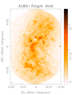
Figure 2: Images of the 3 mm dust continuum emission (in units of mJy beam^-1) toward G0.253+0.016  showing the emission detected in the ALMA-only image (left) and the recovery of the emission on the large spatial scales provided by the inclusion of the zero-spacing information (ALMA + single dish, right). These images are shown in equatorial coordinates: the (0,0) offset position in R.A. and Dec is 17:46:09.59, $-$28:42:34.2 J2000.

The combination of the datasets was performed in CASA via the CLEAN algorithm (see Rathborne et al., 2014a). Figure 2 shows the ALMA-only continuum image (left) and the combined image created using the Herschel  500 $\mu$m  emission assuming a $\beta$ of 1.2 (right). The ALMA-only image clearly shows the image artefacts from the missing flux on large scales, while the combined image shows the significant improvement and recovery of the large scale emission. The removal of the image artefacts justifies the value for $\beta$ $\sim$1.2: higher values underestimate the flux density on large scales which does not remove the zero-spacing imaging artefacts. Thus, we assume $\beta$ of 1.2 $\pm$ 0.1.

Because the 3 mm emission is optically thin and traces all material along the line of sight, it is proportional to the total column density of dust. With T_dust of 20 K and assuming a gas to dust mass ratio of 100, dust absorption coefficient ($\kappa_{3mm}$) of 0.27 cm² g^-1 (using $\kappa_{1.2mm}$ = 0.8 cm² g^-1, and $\kappa\propto\nu^{\beta}$; Chen et al., 2008; Ossenkopf & Henning, 1994), and $\beta$ of 1.2 , the intensity of the emission (I_3mm, in mJy) was converted to column density, N(H₂), by multiplying by 1.9 $\times$ 10²³ ${\rm cm}^{-2}$/mJy. The uncertainties for T_dust and $\beta$ introduce an uncertainty of $\sim$ 10% for the column density, volume density, mass, and virial ratio. In log-normal fits to the N-PDF, there is an uncertainty of $\sim$10% in the dispersion and $\sim$25% for the peak column density.

4 The column density PDF

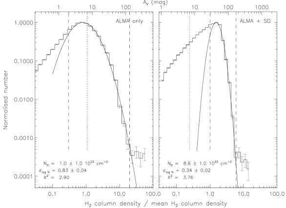
Figure 3: Normalised column density PDFs for G0.253+0.016  (histograms, left: derived using the ALMA-only image, right: derived using the combined image). The error bars show the $\sqrt{number}$ uncertainties. The solid curves are log-normal fits to the PDF: best-fit parameters are labeled. Vertical dashed lines show the fit range (the limits mark the approximate point at which the distributions deviate from log-normal). Vertical dotted lines mark N(H₂)=1.4 $\times$ 10²² ${\rm cm}^{-2}$. The small deviation at the highest column densities traces material that is self-gravitating and corresponds to the only location in the cloud where star formation is occurring.

The sensitivity and angular resolution of the ALMA data allows us to derive the N-PDF for G0.253+0.016  to high accuracy. Figure 3 compares the N-PDF derived from the ALMA-only data to that derived from the combined image (left and right respectively). Both N-PDFs are well fitted by a log-normal distribution. When using the combined image, the shape of the N-PDF remains log-normal, however, the derived dispersion is narrower and the peak column density higher compared to using the ALMA-only image. These differences are expected when including/excluding large scale emission (Schneider et al., 2014).

The deviation from log-normal at low column densities arises from the large-scale diffuse medium and is a common feature in other PDFs (e.g. Lupus I, Pipe, Cor A, see fig. 4 from Kainulainen et al., 2009). Since the ALMA-only image recovers a small fraction of the total flux ($\sim$ 18%), its PDF will characterize the highest contrast peaks within the cloud. Thus, to make meaningful comparisons between the N-PDF for the G0.253+0.016  and to solar neighbourhood clouds and theoretical predictions requires the inclusion of the large-scale emission. Thus, we use the values derived from that N-PDF (i.e. Fig. 3, right) but report both sets of values for completeness.

There is a small deviation from the log-normal distribution at the highest column densities which indicates self-gravitating gas where star formation is commencing. This high-column density material arises from contiguous pixels that exactly coincide with the location of previously-known water maser emission – the only evidence for star formation within the cloud (Lis & Carlstrom, 1994; Kauffmann et al., 2013). Because the immediate vicinity of a forming star is heated, this deviation may result from a higher temperature in this small region rather than a higher column density. Nevertheless, in either case, this deviation from the log-normal distribution indicates the effect of self-gravity.

Assuming a dust temperature of 20 K, we calculate the mass of this core (R$\sim$0.04 pc) to be 72 M_⊙, and its volume density to be $>$3.0 $\times$ 10⁶ ${\rm cm}^{-3}$  (with T_dust=50 K, M=26 M_⊙, and $\rho>$ 1.2 $\times$ 10⁶ ${\rm cm}^{-3}$; the density is a lower limit since this core is unresolved). To assess whether it is gravitationally bound and unstable to collapse or unbound and transient, we determine the virial parameter, $\alpha_{\rm vir}$, defined as $\alpha_{\rm vir}=3k\sigma^{2}R/GM$, where $\sigma$ is the measured 1-dimensional velocity dispersion, $R$ the radius, $G$ the gravitational constant, $M$ the mass, and $k$ is a constant that depends on the density distribution (MacLaren et al., 1988). For high-mass star-forming cores with density profiles $\rho\propto r^{-1.8}$ (Garay et al., 2007), $k$ is 1.16. Because the core’s associated H₂CS molecular line emission is unresolved in velocity, $\sigma$ $<$1.4 km s^-1. Thus, for a mass of 72  M_⊙  $\alpha_{\rm vir}$ $<$ 1.1 (for M=26 M_⊙, $\alpha_{\rm vir}$ $<$ 2.8 ). Since $\alpha_{\rm vir}$ is $\sim$ 1 , this star-forming core is likely gravitationally bound and unstable to collapse.

5 Discussion

5.1 Comparison to solar neighbourhood clouds

In this section we show that both the similarities and differences in the PDFs for solar neighbourhood and CMZ clouds agree with predictions of turbulent models given their environments (for a summary, see Table 1 and references therein).

The similarity in the measured dispersions of the N-PDFs ($\sigma_{\log{N}}$=0.28–0.59 in the solar neighbourhood and 0.34 $\pm$ 0.03 in G0.253+0.016) is understood by considering their turbulent Mach numbers. The gas temperature in the solar neighbourhood and CMZ ($\sim$10 K and $\sim$65 K) correspond to sound speeds ($c_{s}$) of $\sim$ 0.2 and 0.5 km s^-1, respectively. Given the observed velocity dispersions ($\sigma$$\sim$ 2 and $\sim$15 km s^-1  respectively), their $\mathcal{M}_{1{\rm D}}$  numbers are $\sim$10 and $\sim$30, which corresponds to predictions of $\sigma_{\log{\rho}}\sim$ 2.08 and 2.55 for the solar neighbourhood and CMZ respectively (assuming $b$=0.5). Thus, while the $\mathcal{M}_{1{\rm D}}$  for CMZ clouds compared to solar neighbourhood clouds is higher, the predicted values for $\sigma_{\log{\rho}}$ differ by only a factor of 1.2 due to the weak dependence of $\sigma_{\log{\rho}}$ on $\mathcal{M}_{1{\rm D}}$.

The difference in the mean column densities of the N-PDFs ($N_{0}=0.5$–$3.0\times 10^{21}$ ${\rm cm}^{-2}$  in the solar neighbourhood and 86 $\pm$ 20 $\times 10^{21}$ ${\rm cm}^{-2}$  in G0.253+0.016) is understood by considering the relative gas pressures. The turbulent gas pressure is given by $P_{turb}=\rho\,\sigma^{2}$. For typical values for solar neighbourhood ($\rho$$\sim$10² ${\rm cm}^{-3}$; $\sigma$$\sim$2 km s^-1) and CMZ clouds ($\rho$ $\sim$10⁴ ${\rm cm}^{-3}$; $\sigma$$\sim$15 km s^-1), the turbulent gas pressures in units of $P/k$ are 10⁵ and 10⁹ K ${\rm cm}^{-3}$  respectively. The hydrostatic pressure from self gravity ($P_{grav}$) is related to the gas surface density ($\Sigma$) through $P_{grav}=(3/2)\pi G\Sigma^{2}$. Given the surface density of solar neighbourhood ($\Sigma$$\sim$$10^{2}$ M_⊙ pc^-2) and CMZ clouds ($\Sigma$$\sim$$5\times 10^{3}$ M_⊙ pc^-2), the respective hydrostatic pressure in units of $P/k$ are also 10⁵ and 10⁹ K ${\rm cm}^{-3}$. As $P_{turb}\approx P_{grav}$, the pressures are close to equilibrium on the cloud scale for both environments. Because $P_{grav}\sim\Sigma^{2}$, the condition of hydrostatic equilibrium translates the factor of $10^{4}$ difference in turbulent pressure to a factor of $\sim 10^{2}$ difference in column densities. This explains the factor of 10² difference between the mean column density for solar neighbourhood clouds and the CMZ cloud G0.253+0.016.

The conversion of a N-PDF to a $\rho$-PDF has not been solved conclusively. Theoretical work suggests that the conversion is a multiplication by a factor $\xi$, where $\sigma_{\log{\rho}}=\xi\,\sigma_{\log{N}}$ (Brunt et al., 2010). The uncertainty on $\xi$ is $\sim$15%  for the values of $\sigma_{\log{N}}$  measured in solar neighbourhood and CMZ clouds (Brunt et al., 2010)  – smaller than the observed spread of the measured $\sigma_{\log{N}}$. The relative universality of $\xi$ means that the small relative change of the N-PDF dispersions ($[\sigma_{\log{N}}]_{\rm CMZ}\sim[\sigma_{\log{N}}]_{\rm Solar}$) translates to the same relative change of the $\rho$-PDF dispersions, thereby allowing a direct comparison of the measurements to theory. Thus, within the uncertainties, the N-PDF of G0.253+0.016  satisfies the theoretical prediction that $[\sigma_{\log{\rho}}]_{\rm CMZ}\sim[\sigma_{\log{\rho}}]_{\rm Solar}$, providing the first reliable test of turbulence theory in a high-pressure environment. Because we neglected magnetic fields, the similarity in the predicted and measured dispersions suggests that the thermal-to-magnetic pressure ratios (Molina et al., 2012) are also comparable in the solar neighbourhood and the CMZ (and are likely close to unity). However, future observations of the magnetic fields within the high-density material in both environments are needed to confirm this.

5.2 An environmentally dependent star formation threshold

Observations of solar neighbourhood clouds suggest a column density threshold of $\sim$ 1.4 $\times$ 10²² ${\rm cm}^{-2}$, above which star formation proceeds with very high efficiency on a 20 Myr time-scale (Lada et al., 2010). While the exact interpretation has been questioned (Gutermuth et al., 2011; Burkert & Hartmann, 2013) subsequent work suggests a ‘universal’ column density threshold for star formation (Lada et al., 2012). This empirically-motivated universality is at odds with the volume density threshold predicted by theoretical models of turbulence, which depends on $\rho_{0}$ and $\mathcal{M}_{1{\rm D}}$. Despite it accurately describing star formation in solar neighbourhood clouds, this ‘universal’ threshold does not hold for the CMZ: the majority of the gas has N(H₂) $\gg$ 1.4 $\times$ 10²² ${\rm cm}^{-2}$, yet it is forming stars 1–2 orders of magnitude less efficiently than predicted by this threshold (Longmore et al., 2013). The N-PDF for G0.253+0.016  confirms this result. While the majority of the mass has N(H₂) $>$ 1.4 $\times$ 10²² ${\rm cm}^{-2}$, only one region, corresponding to 0.06% of the total mass, shows evidence for star formation (Fig. 3). This result casts doubt on a universal threshold for star formation of N(H₂) $\sim$ 1.4 $\times$10²² ${\rm cm}^{-2}$.

This discrepancy can be understood by considering predictions of theoretical models of turbulent clouds (Krumholz & McKee, 2005; Padoan & Nordlund, 2011). Using the mean volume density and Mach number of the solar neighbourhood ($\rho_{0}$$\sim$10² ${\rm cm}^{-3}$; $\mathcal{M}_{1{\rm D}}$$\sim$10) and CMZ clouds ($\rho_{0}$$\sim$10⁴ ${\rm cm}^{-3}$; $\mathcal{M}_{1{\rm D}}$$\sim$30), the predicted values for $\rho_{crit}$ are $\sim$10⁴ and $\sim$10⁸ ${\rm cm}^{-3}$, respectively. Empirical studies show that, in solar neighbourhood clouds, column densities of 1.4 $\times$ 10²² ${\rm cm}^{-2}$  correspond to volume densities of $\sim$ 10⁴ ${\rm cm}^{-3}$  (suggesting a common size scale of star forming cores of $\sim$0.2 pc; Bergin et al., 2001; Lada et al., 2010). Thus, for the solar neighbourhood, this volume density agrees with the prediction for $\rho_{crit}$.

The sole star-forming core in G0.253+0.016, with a derived volume density $>10^{6}$ ${\rm cm}^{-3}$  conforms to the higher threshold predicted for CMZ clouds. Its associated molecular line emission (from H₂CS) traces very dense gas (i.e. $>$ 10⁷ ${\rm cm}^{-3}$), confirming that $\rho\gg 10^{6}$ ${\rm cm}^{-3}$. While higher resolution observations are required to spatially resolve the core, this derived lower limit is consistent with the theoretically predicted, environmentally dependent volume density threshold – orders of magnitude higher than derived for solar neighbourhood clouds.

5.3 CMZ clouds as local analogues of clouds in the early Universe

Recent surveys have unveiled rapidly ($100$–$1000~{}{\rm M}_{\odot}~{}{\rm yr}^{-1}$) star-forming galaxies (Förster Schreiber et al., 2009; Swinbank et al., 2010; Daddi et al., 2010) at high redshifts ($z>2$), near the peak epoch of star formation (Hopkins & Beacom, 2006). Understanding how these high star formation rates can be achieved is one of the main challenges in galaxy formation. Building upon both their simplicity and success, models of turbulent cloud structure based on solar neighbourhood clouds have been applied to explain the extreme star formation activity in these galaxies (Krumholz et al., 2012; Renaud et al., 2012). However, their low turbulent pressures ($P/k<10^{5}~{}{\rm K}~{}{\rm cm}^{-3}$) differ from their high-redshift counterparts by several orders of magnitude ($P/k>10^{7}~{}{\rm K}~{}{\rm cm}^{-3}$; Swinbank et al., 2011; Kruijssen & Longmore, 2013).

Given the modest metallicity difference between the CMZ and rapidly star-forming, high-redshift galaxies (less than a factor of 2–3; Erb et al., 2006; Longmore et al., 2013), CMZ clouds have the potential to be used as local analogues of clouds in $z>2$ galaxies (Kruijssen & Longmore, 2013). Indeed, CMZ clouds can be studied in a level of detail that is unachievable for clouds at earlier epochs. Our results provide the first empirical evidence that the current theoretical understanding of structure derived from solar neighbourhood clouds also holds in extreme, high-pressure environments. As such, the application of these theories to describe star formation in the early Universe may be valid.

6 Conclusions

Using the new ALMA telescope to obtain high sensitivity 3 mm observations, we have measured the dust column density with an extreme cloud in the CMZ, G0.253+0.016, to high accuracy. Our analysis shows that the log-normal shape, dispersion, and mean of its column density PDF very closely matches the predictions of theoretical models of supersonic turbulence in gas of such high density and turbulence. The lack of wide-spread star formation throughout the cloud, combined with the fact that the PDF shows a small deviation at high-column densities, confirms the youth of G0.253+0.016. Our results are consistent with the theoretically predicted environmentally-dependent threshold for star formation which provides a natural explanation for the low star formation rate in the CMZ (Kruijssen et al., 2014). The confirmation of these models in a high-pressure environment suggests that our current theoretical understanding of gas structure derived from solar neighbourhood clouds may also hold in the early Universe.

Figure 1: Three colour image of G0.253+0.016  (blue is Spitzer  3.6 $\mu$m  emission tracing stars, green is Spitzer  8.0 $\mu$m  emission tracing the bright Galactic background, while red is ALMA 3 mm emission tracing dust from the cloud’s interior; the cloud has an effective radius of 2.9 pc). The position of a water maser is marked, which is evidence for active star formation. The cloud is so cold and dense that it is seen as an extinction feature against the bright IR emission from the Galaxy. Because ALMA sees through to the cloud’s interior, we are now able to characterise its internal structure.

Table 1: Molecular cloud properties within the solar neighbourhood (Solar) and Central Molecular Zone (CMZ). The key properties are marked in bold.

		Solar	CMZ	References
Observed:
	Gas temperature (Tgas)	10 K	65 K	1, 2
	Velocity dispersion ($\sigma$)	2 km s-1	15 km s-1	3, 4, 5
	Average volume density ($\rho$)	102 ${\rm cm}^{-3}$	104 ${\rm cm}^{-3}$	3, 4, 5
	Gas surface density ($\Sigma$)	102 M⊙ pc-2	5$\times 10^{3}$ M⊙ pc-2	6, 5
Derived:
	Sound speed ($c_{s}$)	0.2 km s-1	0.5 km s-1
	Turbulent Mach number ($\mathcal{M}_{1{\rm D}}$)	10	30
	Turbulent gas pressure ($P_{turb}/k$)	105 K ${\rm cm}^{-3}$	109 K ${\rm cm}^{-3}$
	Hydrostatic pressure from self gravity ($P_{grav}/k$)	105 K ${\rm cm}^{-3}$	109 K ${\rm cm}^{-3}$
		Solar	G0.253+0.016
Measured:
	Mean, column density PDF (N0)	0.5–3.0$\times$1021 ${\rm cm}^{-2}$	86 $\pm$ 20 $\times$1021 ${\rm cm}^{-2}$	7, 8
	Dispersion, column density PDF ($\sigma_{\log{N}}$)	0.28–0.59	0.34 $\pm$ 0.03	7, 8
	Critical volume density ($\rho_{crit}$)	104 ${\rm cm}^{-3}$	$>$ 106 ${\rm cm}^{-3}$	3, 9, 8
Predicted (relative to solar neighbourhood clouds):
	Mean, column density PDF (N0)	1	100
	Dispersion, volume density PDF ($\sigma_{\log{\rho}}$)	1	1.2
	Critical volume density ($\rho_{crit}$)	1	104	10, 11, 5

References

- Ao et al. (2013) Ao, Y., Henkel, C., Menten, K. M., Requena-Torres, M. A., Stanke, T., Mauersberger, R., Aalto, S., Mühle, S., & Mangum, J. 2013, A&A, 550, A135
- Ballesteros-Paredes et al. (2011) Ballesteros-Paredes, J., Vázquez-Semadeni, E., Gazol, A., Hartmann, L. W., Heitsch, F., & Colín, P. 2011, MNRAS, 416, 1436
- Bergin et al. (2001) Bergin, E. A., Ciardi, D. R., Lada, C. J., Alves, J., & Lada, E. A. 2001, ApJ, 557, 209
- Brunt et al. (2010) Brunt, C. M., Federrath, C., & Price, D. J. 2010, MNRAS, 405, L56
- Burkert & Hartmann (2013) Burkert, A. & Hartmann, L. 2013, ApJ, 773, 48
- Chen et al. (2008) Chen, X., Launhardt, R., Bourke, T. L., Henning, T., & Barnes, P. J. 2008, ApJ, 683, 862
- Daddi et al. (2010) Daddi, E., Elbaz, D., Walter, F., Bournaud, F., Salmi, F., Carilli, C., Dannerbauer, H., Dickinson, M., Monaco, P., & Riechers, D. 2010, ApJ, 714, L118
- Erb et al. (2006) Erb, D. K., Shapley, A. E., Pettini, M., Steidel, C. C., Reddy, N. A., & Adelberger, K. L. 2006, ApJ, 644, 813
- Federrath et al. (2010) Federrath, C., Roman-Duval, J., Klessen, R. S., Schmidt, W., & Mac Low, M.-M. 2010, A&A, 512, A81
- Förster Schreiber et al. (2009) Förster Schreiber, N. M., Genzel, R., Bouché, N., Cresci, G., Davies, R., Buschkamp, P., Shapiro, K., Tacconi, L. J., Hicks, E. K. S., Genel, S., Shapley, A. E., Erb, D. K., Steidel, C. C., Lutz, D., Eisenhauer, F., Gillessen, S., Sternberg, A., Renzini, A., Cimatti, A., Daddi, E., Kurk, J., Lilly, S., Kong, X., Lehnert, M. D., Nesvadba, N., Verma, A., McCracken, H., Arimoto, N., Mignoli, M., & Onodera, M. 2009, ApJ, 706, 1364
- Garay et al. (2007) Garay, G., Mardones, D., Brooks, K. J., Videla, L., & Contreras, Y. 2007, ApJ, 666, 309
- Goodman et al. (2009) Goodman, A. A., Pineda, J. E., & Schnee, S. L. 2009, ApJ, 692, 91
- Gutermuth et al. (2011) Gutermuth, R. A., Pipher, J. L., Megeath, S. T., Myers, P. C., Allen, L. E., & Allen, T. S. 2011, ApJ, 739, 84
- Hopkins & Beacom (2006) Hopkins, A. M. & Beacom, J. F. 2006, ApJ, 651, 142
- Johnston et al. (2014) Johnston, K. G., Beuther, H., Linz, H., Schmiedeke, A., Ragan, S. E., & Henning, T. 2014, ArXiv e-prints
- Kainulainen et al. (2009) Kainulainen, J., Beuther, H., Henning, T., & Plume, R. 2009, A&A, 508, L35
- Kainulainen et al. (2013) Kainulainen, J., Federrath, C., & Henning, T. 2013, A&A, 553, L8
- Kauffmann et al. (2013) Kauffmann, J., Pillai, T., & Zhang, Q. 2013, ApJ, 765, L35
- Kritsuk et al. (2011) Kritsuk, A. G., Norman, M. L., & Wagner, R. 2011, ApJ, 727, L20
- Kruijssen & Longmore (2013) Kruijssen, J. M. D. & Longmore, S. N. 2013, MNRAS, 435
- Kruijssen et al. (2014) Kruijssen, J. M. D., Longmore, S. N., Elmegreen, B. G., Murray, N., Bally, J., Testi, L., & Kennicutt, R. C. 2014, MNRAS, 440, 3370
- Krumholz et al. (2012) Krumholz, M. R., Dekel, A., & McKee, C. F. 2012, ApJ, 745, 69
- Krumholz & McKee (2005) Krumholz, M. R. & McKee, C. F. 2005, ApJ, 630, 250
- Lada et al. (2012) Lada, C. J., Forbrich, J., Lombardi, M., & Alves, J. F. 2012, ApJ, 745, 190
- Lada et al. (2010) Lada, C. J., Lombardi, M., & Alves, J. F. 2010, ApJ, 724, 687
- Larson (2003) Larson, R. B. 2003, Reports on Progress in Physics, 66, 1651
- Lis & Carlstrom (1994) Lis, D. C. & Carlstrom, J. E. 1994, ApJ, 424, 189
- Lis & Menten (1998) Lis, D. C. & Menten, K. M. 1998, ApJ, 507, 794
- Lis et al. (2001) Lis, D. C., Serabyn, E., Zylka, R., & Li, Y. 2001, ApJ, 550, 761
- Lombardi et al. (2008) Lombardi, M., Lada, C. J., & Alves, J. 2008, A&A, 489, 143
- Longmore et al. (2013) Longmore, S. N., Bally, J., Testi, L., Purcell, C. R., Walsh, A. J., Bressert, E., Pestalozzi, M., Molinari, S., Ott, J., Cortese, L., Battersby, C., Murray, N., Lee, E., Kruijssen, J. M. D., Schisano, E., & Elia, D. 2013, MNRAS, 429, 987
- Longmore et al. (2014) Longmore, S. N., Kruijssen, J. M. D., Bastian, N., Bally, J., Rathborne, J., Testi, L., Stolte, A., Dale, J., Bressert, E., & Alves, J. 2014, ArXiv e-prints
- Longmore et al. (2012) Longmore, S. N., Rathborne, J., Bastian, N., Alves, J., Ascenso, J., Bally, J., Testi, L., Longmore, A., Battersby, C., Bressert, E., Purcell, C., Walsh, A., Jackson, J., Foster, J., Molinari, S., Meingast, S., Amorim, A., Lima, J., Marques, R., Moitinho, A., Pinhao, J., Rebordao, J., & Santos, F. D. 2012, ApJ, 746, 117
- MacLaren et al. (1988) MacLaren, I., Richardson, K. M., & Wolfendale, A. W. 1988, ApJ, 333, 821
- Molina et al. (2012) Molina, F. Z., Glover, S. C. O., Federrath, C., & Klessen, R. S. 2012, MNRAS, 423, 2680
- Morris & Serabyn (1996) Morris, M. & Serabyn, E. 1996, ARA&A, 34, 645
- Motte et al. (1998) Motte, F., Andre, P., & Neri, R. 1998, A&A, 336, 150
- Ossenkopf & Henning (1994) Ossenkopf, V. & Henning, T. 1994, A&A, 291, 943
- Padoan et al. (2013) Padoan, P., Federrath, C., Chabrier, G., Evans, II, N. J., Johnstone, D., Jørgensen, J. K., McKee, C. F., & Nordlund, Å. 2013, ArXiv e-prints
- Padoan & Nordlund (1999) Padoan, P. & Nordlund, Å. 1999, ApJ, 526, 279
- Padoan & Nordlund (2011) —. 2011, ApJ, 730, 40
- Rathborne et al. (2014a) Rathborne, J. M., Longmore, S. N., Jackson, J. M., Alves, J., Bally, J., Bastian, N., Bressert, E., Contreras, Y., Foster, J. B., Garay, G., Kruijssen, J. M. D., Testi, L., & Walsh, A. J. 2014a, ApJ submitted
- Rathborne et al. (2014b) Rathborne, J. M., Longmore, S. N., Jackson, J. M., Foster, J. B., Contreras, Y., Garay, G., Testi, L., Alves, J. F., Bally, J., Bastian, N., Kruijssen, J. M. D., & Bressert, E. 2014b, ApJ, 786, 140
- Renaud et al. (2012) Renaud, F., Kraljic, K., & Bournaud, F. 2012, ApJ, 760, L16
- Schneider et al. (2014) Schneider, N., Ossenkopf, V., Csengeri, T., Klessen, R., Federrath, C., Tremblin, P., Girichidis, P., Bontemps, S., & Andre, P. 2014, ArXiv e-prints
- Swinbank et al. (2011) Swinbank, A. M., Papadopoulos, P. P., Cox, P., Krips, M., Ivison, R. J., Smail, I., Thomson, A. P., Neri, R., Richard, J., & Ebeling, H. 2011, ApJ, 742, 11
- Swinbank et al. (2010) Swinbank, A. M., Smail, I., Longmore, S., Harris, A. I., Baker, A. J., De Breuck, C., Richard, J., Edge, A. C., Ivison, R. J., Blundell, R., Coppin, K. E. K., Cox, P., Gurwell, M., Hainline, L. J., Krips, M., Lundgren, A., Neri, R., Siana, B., Siringo, G., Stark, D. P., Wilner, D., & Younger, J. D. 2010, Nature, 464, 733
- Vázquez-Semadeni (1994) Vázquez-Semadeni, E. 1994, ApJ, 423, 681
- Walmsley et al. (1986) Walmsley, C. M., Guesten, R., Angerhofer, P., Churchwell, E., & Mundy, L. 1986, A&A, 155, 129