Multiple Access for Small Packets Based on Precoding and Sparsity-Aware Detection

Abstract

Modern mobile terminals often produce a large number of small data packets. For these packets, it is inefficient to follow the conventional medium access control protocols because of poor utilization of service resources. We propose a novel multiple access scheme that employs block-spreading based precoding at the transmitters and sparsity-aware detection schemes at the base station. The proposed scheme is well suited for the emerging massive multiple-input multiple-output (MIMO) systems, as well as conventional cellular systems with a small number of base-station antennas. The transmitters employ precoding in time domain to enable the simultaneous transmissions of many users, which could be even more than the number of receive antennas at the base station. The system is modeled as a linear system of equations with block-sparse unknowns. We first adopt the block orthogonal matching pursuit (BOMP) algorithm to recover the transmitted signals. We then develop an improved algorithm, named interference cancellation BOMP (ICBOMP), which takes advantage of error correction and detection coding to perform perfect interference cancellation during each iteration of BOMP algorithm. Conditions for guaranteed data recovery are identified. The simulation results demonstrate that the proposed scheme can accommodate more simultaneous transmissions than conventional schemes in typical small-packet transmission scenarios.

I Introduction

As intelligent terminals such as smart phones and tablets get more popular, they produce an increasing number of data packets of short lengths, to be delivered over a cellular network. Modern mobile applications that produce such small packets include instant messaging, social networking, and other services [1],[2]. Although the lengths of messages are relatively short, small packet services put great burden on the communication network. Two kinds of messages contribute to the traffic of small packets: one is the small packets of conversation produced by active users that occupy only a small percentage of the total online users [2]; the other is the signaling overheads needed to transmit these conversation packets [3].

In current wireless communication systems, a user follows the medium access control (MAC) protocols to obtain the service resources. Two flavors of MAC protocols are used in general: i) resource reservation based, and ii) collision resolution based. In the first kind, resources are preallocated to the users in a noncompetitive fashion. For small and random packets, the reservation-based approach is inefficient in resource utilization due to irregularity of the packets. In the collision-resolution based approaches, the terminals are allowed to access the resources in arbitrary order and when collision occurs, certain resolution mechanism is then employed. The collision-resolution based MAC can suffer from too many retransmissions due to frequent collisions.

In this paper, we propose a novel uplink small packet transmission scheme based on precoding at the transmitters and sparsity-aware detection at the receiver. The main motivation is to allow for a large number of users to transmit simultaneously, although each user may be transmitting only a small amount of data. Besides frame-level synchronization, no competition for resources or other coordinations are required. This saves the signaling overhead for collision resolution, and improves the resource utilization efficiency.

The contributions of our work are as follows:

1. Block precoding and block-sparse system modeling: We apply block precoding at each transmitter in time domain, and by considering the user activities, develop a block-sparse system model that takes full advantages of the structure of the signals to recover and is suitable for compressive-sensing based detection algorithms.

2. Sparsity-aware detection algorithm: We develop a interference cancellation (IC) based block orthogonal matching pursuit (ICBOMP) algorithm. The algorithm improves upon the traditional BOMP algorithm by taking advantage of availability of error correction and detection, which is common in digital communications. By ICBOMP algorithm, not only do we achieve much better signal recovering accuracy but we also benefit in terms of less computational complexity. The price is slightly decreased rate due to coding.

3. Signal recovery conditions: We derive conditions for guaranteed signal recovery. The condition we require on the BOMP algorithm is milder than that in the related work in [20]. For ICBOMP algorithm, we give the conditions for perfect IC in each iteration. Furthermore, we characterize the data recovery condition from information theoretic point of view.

Thanks to the precoding operation and our sparsity-aware detection algorithms, our scheme enable the system to support more active users to be simultaneously served. The number of active users can be even more than the number of antennas at base station (BS). This is of great practical significance for networks offering small packet services to a large number of users.

Our proposed scheme is especially suitable for the so called massive multiple-input multiple-output (MIMO) systems [7]-[10]. In massive MIMO systems, the number of antennas at the BS can be more than the number of active single-antenna users that are simultaneously served. When the number of antennas at BS is large, the different propagation links from the users to the BS tend to be orthogonal, and the large amount of spatial degrees of freedom are useful for mitigating the effect of fast fading [8],[9]. Overall, massive MIMO technique provides higher data rate, better spectral and energy efficiencies [10].

Applications of compressive sensing (CS) to random MAC channels have been considered in [22]-[25]. In [22], CS based decoding scheme at the BS has been used for the multiuser detection task in asynchronous random access channels. A technique based on CS for meter reading in smart grid is proposed in [23], and its consideration is limited to single-antenna systems. Besides, a novel neighbor discovery method in wireless networks with Reed-Muller Codes has been proposed in [25], where CS technique is also adopted. All the referred works depend on the idea that the MAC channel is sparse, and all their works are classified to initial category of CS, where no structure property have been taken into account. This is one of the main distinctions that differentiate our work from the referred ones.

The rest of the paper is organized as follows. In Section II, the system model of block sparsity are given. In Section III, we introduce the BOMP algorithm and its improved version ICBOMP algorithm to recover the transmitted signals. Guarantees for data recovery are presented in Section IV. Section V will present the numerical experiments that prove the effectiveness of our scheme. Afterwards, to invest the scheme with practical significance, some issues are discussed in Section VI. Finally, the conclusion will be presented in Section VII. To better organize the contents, we will relegate some of the proofs to the appendix.

Notation: Vectors and matrices are denoted by boldface lowercase and uppercase letters, respectively. The 2-norm of a vector ${\mathbf{v}}$ is denoted as ${\|{\mathbf{v}}\|_{2}}$, and the 0-norm is given as ${\|{\mathbf{v}}\|_{0}}$. The inner product of two vectors ${\mathbf{v}}_{1}$ and ${\mathbf{v}}_{2}$ is denoted as $({{{\mathbf{v}}_{1}},{{\mathbf{v}}_{2}}})$. The identity matrix of $d\times d$ dimension is denoted as ${\mathbf{I}}_{d}$. For a given matrix ${\mathbf{U}}$, its conjugate transpose, transpose, pseudo inverse, trace and rank are respectively denoted as ${\mathbf{U}}^{H}$, ${\mathbf{U}}^{T}$, ${{\mathbf{U}}^{\dagger}}$, $\text{Tr}\{{\mathbf{U}}\}$, $\text{rank}\{{\mathbf{U}}\}$, and the spectral norm of ${\mathbf{U}}$ is given by $\|{\mathbf{U}}\|$. Operation $vec({\mathbf{U}})$ denotes vectorizing ${\mathbf{U}}$ by column stacking. For a subset $I\subset[N]:=\{1,2,\cdots,N\}$ and matrix ${\mathbf{U}}:=[{{{\mathbf{U}}_{1}},{{\mathbf{U}}_{2}},\cdots,{{\mathbf{U}}_{N}}}]$ consisting of $N$ sub-matrices (blocks), where each sub-matrix has equal dimensionality, ${\mathbf{U}}_{I}$ denotes a sub-matrix of ${\mathbf{U}}$ with block indices in $I$; for a vector ${\mathbf{v}}:={[{{\mathbf{v}}_{1}^{T},{\mathbf{v}}_{2}^{T},\cdots,{\mathbf{v}}_{N}^{T}}]^{T}}$, ${\mathbf{v}}_{I}$ is similarly defined. For a set $A$, $|A|$ denotes its cardinality. For two sets $A$ and $B$, $A\backslash B:=A\cap B^{c}$ denotes the set difference. For a real number $r$, $|r|$ and $\text{Re}(r)$, and $\lfloor r\rfloor$ denote its absolute value, real part, and floor, respectively. Operation $\otimes$ denotes the Kronecker product of two matrices.

II System Model

Consider an uplink system with $N$ mobile users, each with a single antenna, and a BS with $M$ antennas. When a terminal is admitted to the network, it becomes an online user. We assume that there are $N_{a}$ active users, out of the total $N$ online users, that have data to transmit. It is not required $N_{a}$ be known a priori or ${N_{a}}<M$; actually, in practical systems $N_{a}$ is usually unknown and it is possible that $N_{a}\gg M$.

We make the following further assumptions on the system considered.

1. The channels are block-fading: it remains constant for a certain duration and then changes independently.

2. The transmissions are in blocks and the users are synchronized at the block level. We assume that each frame of transmission consists of $T$ symbols, which all fall within one channel coherent interval.

3. The users each have single antenna. There are multiple antennas at the BS.

4. The antennas at the BS, as well as the antennas among users, are uncorrelated and uncoupled.

5. The BS always has perfect channel state information (CSI) of online users.

Let ${\mathbf{s}}_{n}\in{\mathbb{C}^{d\times 1}}$ denotes the symbols to be transmitted by user $n$, with $d<T$. User $n$ applies a precoding to ${\mathbf{s}}_{n}$ to yield

$${{\mathbf{x}}_{n}}={{\mathbf{P}}_{n}}{{\mathbf{s}}_{n}}$$ (1)

where ${\mathbf{P}}_{n}$ is a complex precoding matrix of size $T\times d$. The entries of ${\mathbf{x}}_{n}$ are transmitted in $T$ successive time slots. The received signals at all antennas within one frame can be written as

$${\mathbf{Y}}=\sqrt{{\rho_{0}}}\sum_{n=1}^{N}{{{\mathbf{h}}_{n}}{\mathbf{x}}_{n}^{T}}+{\mathbf{Z}}=\sqrt{{\rho_{0}}}\sum_{n=1}^{N}{{{\mathbf{h}}_{n}}{\mathbf{s}}_{n}^{T}{{\mathbf{P}}_{n}^{T}}}+{\mathbf{Z}}$$ (2)

where ${\rho_{0}}$ is the signal to noise ratio (SNR) of the uplink, ${\mathbf{Y}}$ is noisy measurement of size $M\times T$, ${\mathbf{Z}}\in{\mathbb{C}^{M\times T}}$ represents the additive noise, with i.i.d. circularly symmetric complex Gaussian distributed random entries of zero mean and unit variance, and ${\mathbf{h}}_{n}\in{\mathbb{C}^{M\times 1}}$ represents the channel coefficients from the user $n$ to the base station, without loss of generally, let ${h_{mn}}\sim{\mathcal{CN}}({0,1})$, $m=1,2,\cdots,M$. Using the linear algebra identity $vec({{\mathbf{A}}{\mathbf{B}}{\mathbf{C}}})=({{{\mathbf{C}}^{T}}\otimes{\mathbf{A}}})vec({\mathbf{B}})$, we can rewrite the received signal as

$$vec({\mathbf{Y}})=\sqrt{{\rho_{0}}}\sum_{n=1}^{N}{({\mathbf{P}}_{n}\otimes{{\mathbf{h}}_{n}}){{\mathbf{s}}_{n}}}+vec({\mathbf{Z}})$$ (3)

Define ${\mathbf{y}}:=vec({\mathbf{Y}})$, ${{\mathbf{B}}_{n}}:=({{\mathbf{P}}_{n}\otimes{{\mathbf{h}}_{n}}})/\sqrt{M}$ and ${\mathbf{B}}:=[{{{\mathbf{B}}_{1}},{{\mathbf{B}}_{2}},\cdots,{{\mathbf{B}}_{N}}}]$, ${\mathbf{s}}:={[{{\mathbf{s}}_{1}^{T},{\mathbf{s}}_{2}^{T},\cdots,{\mathbf{s}}_{N}^{T}}]^{T}}$. Then we can write the model in (3) as

$${{\mathbf{y}}}=\sqrt{{\rho_{0}}M}{{\mathbf{B}}}{{\mathbf{s}}}+{\mathbf{z}}$$ (4)

In this formulation, we have assumed that all the users have messages of equal length $d$. This may not be the case in practice. We view $d$ as the maximum length of the messages of all users within a frame. For the users whose message length is less than $d$, we assume their messages have been zero-padded to $d$ before precoding. Also, for those users that are not active, we assume their transmitted symbols are all zeros.

Model (4) indicates that the signals to recover present the structure of block-sparsity where transmitted signals are only located in a small fraction of blocks and all other blocks are zeros. The length of each block is $d$. We collect all the indices of blocks corresponding to active users to form a set $I$, with $|I|=N_{a}\leq K$, which means the unknown number of nonzero blocks (active users) is at most $K$. Our consideration is limited to case $MT<Nd$, where (4) represents an under-determined system. For case where $MT>Nd$, the receiver design is easier and the proposed method is also applicable. When precoding matrix ${{\mathbf{P}}_{n}}$ is reasonably designed, matrix ${{\mathbf{B}}}$ can meet the requirement for sensing matrix in CS, and this kind of ${{\mathbf{P}}_{n}}$ is of wide range, for instance, Gaussian or Bernoulli matrix. Therefore, model (4) can be viewed as block sparsity model in CS [19, 20]. In CS, ${{\mathbf{B}}}$ is referred as dictionary.

Remark 1: The following are several remarks on our precoding scheme:

1. The precoding scheme is proposed because in reality, $T$ is usually several times longer than the lengths of small packets. Also, the precoding scheme contributes to solving signal recovery problem in the situation where $N_{a}>M$.

2. Each user knows its own precoding matrix and the BS knows all precoding matrices of all users.

3. A basic requirement on the precoding matrix is that it should be full column rank, which is a requirement for data recovery. Additionally, in order to balance the power of every symbol of the messages before and after being precoded, each column of ${{\mathbf{P}}_{n}}$ should be normalized to unit energy.

4. Our precoding scheme is different from spreading schemes in [23], [24], where direct sequence spread spectrum (DSSS) is utilized for CS formulation.

III Algorithms For Data Recovery

The past few years have also witnessed the research interest in CS [11, 12, 13, 14]. Initial works in CS treat sparse weighting coefficients as just randomly located among possible positions in a vector. When structure of the sparse signal is exploited, for example block sparsity, it is possible to obtain better signal reconstruction performance and reduce the number of required measurements [15, 19, 20, 21].

We develop detection algorithms to be used at the BS in this section. We first apply known algorithm BOMP to our problem, and then further improve it by incorporating IC based on error correction and detection.

III-A BOMP Algorithm

The main idea of BOMP algorithm is that, for each iteration, it chooses a block which has the maximum correlation with the residual signal, and after that, it will use the selected blocks to approximate the original signals by solving a least squares problem [20]. For later convenience, we present the details of BOMP algorithm as follows:

1. Input: Matrix ${{\mathbf{B}}}$, signal vector ${\mathbf{y}}$, ${\rho_{0}}$, $M$, $T$ and $d$.

2. Parameter setting: Maximum number of iterations $K$. Usually, $K\leq\lfloor\frac{MT}{d}\rfloor$. With $K$ iterations, at most $K$ active users can be identified.

3. Initialization: Index set ${{\Lambda}_{t}}=\O$, basis function set ${\mathbf{\Theta}_{0}}=\O$, residual signal ${{\mathbf{r}}_{0}}={\mathbf{y}}$, the number of iterations $t=1$.

4. Main iteration: While $t\leq K$, do the following

   1. Calculate the of correlation coefficients given by the residual signal with each column of ${{\mathbf{B}}}$, denoting as ${{{\mathbf{B}}}^{H}}{{\mathbf{r}}_{t-1}}$.

   2. Find the index ${\lambda_{t}}\in\{{1,2,\ldots,N}\}$ of the block and the block unit ${\mathbf{B}}_{{\lambda_{t}}}$ of ${{\mathbf{B}}}$, satisfying $\{{{\lambda_{t}},{\mathbf{B}}_{\lambda_{t}}}\}=\arg\max_{j\in\{{1,\cdots,N}\}}{\|{{{\mathbf{B}}_{j}^{H}}{{\mathbf{r}}_{t-1}}}\|_{2}}$.

   3. Augment the index set and basis function set, and set the ${\lambda_{t}}$-th block of ${{\mathbf{B}}}$ a zero sub-matrix

      $${{\Lambda}_{t}}={{\Lambda}_{t-1}}\cup\{{\lambda_{t}}\}$$

      $$\mathbf{\Theta}_{t}=[{{\mathbf{\Theta}_{t-1}},{\mathbf{B}}_{\lambda_{t}}}]$$

      $${\mathbf{B}}_{\lambda_{t}}={\mathbf{0}}$$

   4. Estimate the updated signals by least square (LS) algorithm

      $${{\bar{\mathbf{s}}}_{t}}=\arg\max_{{{\mathbf{s}}_{0}}}{\|{{\mathbf{y}}-\sqrt{{\rho_{0}}M}{\mathbf{\Theta}_{t}}{{\mathbf{s}}_{0}}}\|_{2}}$$

   5. Update the residual signals and the iteration number

      $${{\mathbf{r}}_{t}}={\mathbf{y}}-\sqrt{{\rho_{0}}M}{\mathbf{\Theta}_{t}}{{\overline{{\mathbf{s}}}}_{t}}$$

      $$t=t+1$$

5. Output: ${{\bar{\mathbf{s}}}_{K}}$, which is the approximation most unlikely all-zero blocks corresponding to block index set ${\Lambda_{K}}$ in the original block-sparse signal vector ${\mathbf{s}}$.

After we get the approximation of block-sparse coefficients, we can recover the original signals we want.

III-B ICBOMP Algorithm

In addition to the block structure of the signals to recover, the amplitude of each modulated symbol has constant modulus, which could potentially be utilized for improved performance. More importantly, error correction coding is usually used for correcting demodulation errors due to noise and channel disturbances. Error detection codes such as cyclic redundancy check (CRC) codes can be utilized to indicate whether the decoded packets are indeed correct. Such detection cannot be perfect. However, for simplicity we will assume CRC detection is perfect, i.e., the probabilities of miss detection and false alarm are both zero.

Here we propose an improved algorithm ICBOMP which make use of channel coding and CRC to carry out perfect IC in each iteration of BOMP algorithm. The idea of IC can be found in [16, 17, 18].

Let ${\bar{\mathbf{s}}}_{t}^{i}$ denote each $d$-length block ${\bar{\mathbf{s}}}_{t}^{i}$ of ${\bar{\mathbf{s}}}_{t}$, which is obtained by step 4d) in BOMP algorithm, $1\leq i\leq t$. We assume that the transmitters have used certain error correction and detection scheme for each block signal, denoted by $[{\tilde{\Lambda}}_{t},{\tilde{\mathbf{s}}}_{t}]={\mathcal{D}}({\bar{\mathbf{s}}}_{t},d)$, in which ${\tilde{\mathbf{s}}}_{t}$ is the output of input ${\bar{\mathbf{s}}}_{t}$, and each of its blocks is denoted by ${\tilde{\mathbf{s}}}_{t}^{i}$; ${\tilde{\Lambda}}_{t}$ denotes the index set for error-free blocks. For each block, it will go through one of the two distinct operations given by function ${\mathcal{D}}$:

1. If ${\bar{\mathbf{s}}}_{t}^{i}$ after operation of certain channel coding scheme is error-free, then output ${\tilde{\mathbf{s}}}_{t}^{i}$ is its corrected signal vector.

2. If ${\bar{\mathbf{s}}}_{t}^{i}$ after operation of certain channel coding scheme is not error-free, then ${\tilde{\mathbf{s}}}_{t}^{i}={\bar{\mathbf{s}}}_{t}^{i}$.

In ICBOMP algorithm, most of the calculation processes remain the same as BOMP algorithm, and the difference occurs after signals have been updated by LS method in step 4d) of BOMP algorithm, turning residual signals updating steps to the following

$$[{\tilde{\Lambda}}_{t},{\tilde{\mathbf{s}}}_{t}] ={\mathcal{D}}({\bar{\mathbf{s}}}_{t},d)$$ (5)

$${\mathbf{r}}_{t} ={\mathbf{y}}-\sqrt{\rho_{0}M}{\mathbf{B}}_{\Lambda_{t}}{\tilde{\mathbf{s}}}_{t}$$ (6)

$$\Lambda_{t} =\Lambda_{t}\backslash\{{\tilde{\Lambda}}_{t}\}$$ (7)

$$t =t+1$$ (8)

From the above steps, we can see that, when some blocks of signals have been exactly recovered, ICBOMP algorithm regards them as interference signals to the following iterations and eliminates these signals, as well as their contributions to signal receiving model of (4). While for the signal blocks with errors that cannot be corrected, ICBOMP algorithm leaves them as they were obtained through BOMP algorithm. In the case where no error-free block is available, ICBOMP behaves the same way as BOMP.

IV Data Recovery Guarantees

In this section, we will present conditions that guarantee data recovery. Before analyzing conditions for data recovery, some notation and definitions will be introduced first. From the definition of ${{\mathbf{B}}}$, we can see that each column of it is statistically normalized to one. Here we expand ${{\mathbf{B}}}$ as

$${{\mathbf{B}}}=[{\underbrace{{\mathbf{b}_{1}}\cdots{\mathbf{b}_{d}}}_{{\mathbf{B}}_{1}}\underbrace{{\mathbf{b}_{d+1}}\cdots{\mathbf{b}_{2d}}}_{{\mathbf{B}}_{2}}\cdots\underbrace{{\mathbf{b}_{({N-1})d+1}}\cdots{\mathbf{b}_{Nd}}}_{{\mathbf{B}}_{N}}}]$$ (9)

As in [19], [20], we give the definitions of block-coherence as

$${\mu_{\mathbf{B}}}:=\frac{1}{d}\max_{i\neq j}\|{{\mathbf{B}}_{i}^{H}}{\mathbf{B}}_{j}\|$$ (10)

and sub-coherence as

$$\nu:=\max_{1\leq l\leq N}\max_{({l-1})d+1\leq i\neq j\leq ld}|{\mathbf{b}_{i}^{H}{\mathbf{b}_{j}}}|$$ (11)

At the same time define

$${{s_{l}}}:=\min_{{i\in I}}{\|{{\mathbf{s}}_{i}}\|_{2}},\quad{{s_{u}}}:=\max_{{i\in I}}{\|{{\mathbf{s}}_{i}}\|_{2}}$$ (12)

IV-A Data Recovery Conditions For BOMP Algorithm

The following theorem characterizes the block-sparse data recovery performance by BOMP algorithm.

Theorem 1.

Consider the block-sparse model in (4), suppose that condition

$$\begin{split}\rho_{0}M[{1-({d-1})\nu}]^{2}s_{l}^{2}&>\tau^{2}+\rho_{0}Md\mu_{\mathbf{B}}\{2(N_{a}-1)[1+(d-1)\nu]+N_{a}^{2}d\mu_{\mathbf{B}}\}s_{l}^{2}\\ &\quad+2\sqrt{\rho_{0}M}\tau\{(2N_{a}-1)d\mu_{\mathbf{B}}+[1+(d-1)\nu]\}s_{l}\end{split}$$ (13)

is satisfied, then the BOMP algorithm identifies the correct support of signal vector ${\mathbf{s}}$ and at the same time achieves a bounded error given by

$$\|{\hat{\mathbf{s}}}-{\mathbf{s}}\|_{2}^{2}\leq\frac{K\tau^{2}}{[{1-({d-1})\nu-({K-1})d{\mu_{{\mathbf{B}}}}}]^{2}\rho_{0}M}$$ (14)

where ${\hat{\mathbf{s}}}$ is the signal vector recovered by BOMP algorithm, $K\leq\lfloor\frac{MT}{d}\rfloor$ is the maximum number of iterations for BOMP algorithm, $1-(d-1)\nu-(K-1)d\mu_{\mathbf{B}}>0$ and $\tau=\max_{1\leq j\leq N}\|{\mathbf{B}}_{j}^{H}{\mathbf{z}}\|_{2}$. For circularly symmetric complex Gaussian noise ${\mathbf{z}}$,

$$P\{{\tilde{\tau}}\geq\|{\mathbf{B}}_{j}^{H}{\mathbf{z}}\|_{2}\}\geq 1-e^{-\varsigma^{2}}\sum_{k=0}^{d-1}\frac{({{\varsigma^{2}}})^{k}}{k!}$$ (15)

where $\varsigma={\tilde{\tau}}/\sqrt{1+({d-1})\nu}$.

For a certain modulation constellation, suppose that each symbol’s energy has been normalized, and the minimum distance between different symbols is ${l_{\min}}$, for example, ${l_{\min}}=\sqrt{2}$ for quadrature phase shift keying (QPSK) and ${l_{\min}}=2$ for binary phase shift keying (BPSK), then by the bounded error in (14), we can conclude that the number of erroneously demodulated symbols is at most ${N_{e}}=\lfloor{\|{{\hat{\mathbf{s}}}-{\mathbf{s}}}\|_{2}^{2}/{{({{l_{\min}}/2})}^{2}}}\rfloor$. By now, we can present the expression of symbol error rate (SER) as

$$P_{\text{SER}}\leq\frac{N_{e}}{{N_{a}}d}$$ (16)

Remark 2: Since ${T}>d$ and $M{T}\gg d$, we can design orthogonal columns for precoding matrix ${{\mathbf{P}}_{n}}$ of user $n$, $n=1,2,\cdots,N$, then each block of dictionary ${{\mathbf{B}}}$ is sub-matrix with orthogonal columns, meaning $\nu=0$. On the other hand, we have $\tau\gg{{s_{l}}}$ when each nonzero element of ${\mathbf{s}}_{n}$ satisfies a reasonable power constrain. Additionally, if ${\mu_{\mathbf{B}}}=0$, then condition (13) can be simplified as ${{\rho_{0}}M}{{{s_{l}^{2}}}}>{\tau^{2}}+2\sqrt{{\rho_{0}}M}\tau{{s_{l}}}\approx{\tau^{2}}$, which is milder when compared with [20, Theorem 5], which yields ${{\rho_{0}}M}{{{s_{l}^{2}}}}>4{\tau^{2}}$ when applied to our scenario.

IV-B Conditions For Perfect IC In ICBOMP algorithm

Thanks to the error correction and detection, ICBOMP algorithm provides better performance than BOMP algorithm. In the case of perfect IC, the algorithm improves signal recovery quality and also reduces computational complexity. By eliminating the correctly decoded blocks and their contributions, the dimensionality of useful signals is reduced, which contributes to reducing the computations required in matrix inversion of LS algorithm. In the following, we present a theorem that characterizes the conditions for perfect IC in each iteration of ICBOMP algorithm.

When the first $i-1$ iterations and block selection in $i$-th iteration have been finished, suppose $N_{ic}^{i-1}$ blocks of active users are already correctly recovered and cancelled by the previous $i-1$ iterations, and $N_{i}$ blocks, whose indices are gathered to form a set $I^{i}$, will be substituted into least square operation in $i$-th iteration, $N_{ic}^{i-1}+N_{i}=i$. Additionally, let set $I_{u}^{i}$ contain the indices of unidentified active users and set $I_{ic}^{i-1}$ contain the indices of active users that are already successfully recovered and cancelled. Then the following result holds

Theorem 2.

If conditions

$$\begin{split}\rho_{0}M[1-(d-1)\nu_{i}]^{2}s_{il}^{2}&>\tau_{i}^{2}+{\rho_{0}}Md\mu_{i{\mathbf{B}}}\{2(N_{i}-1)[1+(d-1)\nu_{i}]+N_{i}^{2}d\mu_{i{\mathbf{B}}}\}s_{il}^{2}\\ &\quad+2\sqrt{\rho_{0}M}\tau_{i}\{(2N_{i}-1)d\mu_{i{\mathbf{B}}}+[1+(d-1)\nu_{i}]\}s_{il}\end{split}$$ (17)

and

$$[1-(d-1)\nu_{i}-(N_{i}-1)d\mu_{i{\mathbf{B}}}]^{2}\rho_{0}Mt_{c}l_{\min}^{2}\geq 4\tau_{i}^{2}$$ (18)

are satisfied, then at least one block will been successfully recovered and cancelled in $i$-th iteration of ICBOMP algorithm. In (17) and (18), $t_{c}$ is the number of bits that can be corrected by the channel coding scheme,

$$\tau_{i}=\max_{j\in\{[N]\backslash\{I_{IC}^{i-1}\cup I_{c}^{i}\}\}}{\|{\mathbf{B}}_{j}^{H}(\sqrt{\rho_{0}M}{\mathbf{B}}_{I_{c}^{i}}{\mathbf{s}}_{I_{c}^{i}}+{\mathbf{z}})\|_{2}}$$ (19)

and $\mu_{i{\mathbf{B}}}$, $\nu_{i}$ and $s_{il}$ are respectively defined as $\mu_{{\mathbf{B}}}$, $\nu$ and $s_{l}$, and their definitions are only limited to users or active users in $\{[N]\backslash\{I_{ic}^{i-1}\cup I_{u}^{i}\}\}$.

In Theorem 2, we only considered the case where all blocks in $I^{i}$ correspond to active users, based on the consideration that if signals of an active user cannot be successfully recovered when all the active users have been identified, they are less likely to be successfully recovered when non-active blocks begin to enter into the least square algorithm.

Proof:

Theorem 2 can be viewed as a corollary of Theorem 1.

When we consider each iteration in ICBOMP algorithm, by (17) which yields (35) in Appendix A, when applied to $i$-th iteration, the most likely active users will be identified. Treat the users in $I_{u}^{i}$ and noise as perturbations for recovering the signal of users in $I^{i}$. With the same proof for Theorem 1, (17) can be verified. When (17) is satisfied, we achieve an error bounded by

$$\|{\hat{\mathbf{s}}}_{I^{i}}-{\mathbf{s}}_{I^{i}}\|_{2}^{2}\leq\frac{N_{i}\tau_{i}^{2}}{[1-(d-1)\nu_{i}-(N_{i}-1)d\mu_{i{\mathbf{B}}}]^{2}\rho_{0}M}$$ (20)

where we have utilized the knowledge $|I^{i}|=N_{i}$ which can be exactly obtained by ICBOMP algorithm. If condition

$$\|{\hat{s}}_{I^{i}}-s_{I^{i}}\|_{2}^{2}\leq N_{i}t_{c}(\frac{l_{\min}}{2})^{2}$$ (21)

holds, then by correction of channel coding, at least one user’s signals will surely be recovered without an error. By (21), (18) is obtained. ∎

IV-C Condition From Information Theoretic Point Of View

From the BS’s point of view, it is desirable to recover all the information conveyed by ${\mathbf{s}}$, including number of active users, exact indices of these active users, their transmitted information bits, etc.. When all the information are measured by bits, then The number of bits representing the indices of active users and signal bits of the transmitted messages are respectively $\log_{2}\binom{N}{N_{a}}$ and $\sum_{i=1}^{N_{a}}b_{i}$. Assume all bits are generated with equal probability, and let $S$ denote the set of bits needed to represent the total information, then

$$|S|\geq\log_{2}\binom{N}{N_{a}}+\sum_{i=1}^{N_{a}}b_{i}$$ (22)

Remark 3: When the number of active users and lengths of the messages of active users are not prior known to BS, then the inequality in (22) is strictly established. Even when these two factors are prior known to BS, (22) still holds.

The following theorem roughly shows that the total bits of all information that can be recovered at the receiver can not exceed the capability of channel in a frame time.

Theorem 3.

Define $p_{e}$ as the probability that some error has happened in the recovery of the information in set $S$, Then the following condition is necessary for the data recovery

$$|S|\leq\frac{1}{1-p_{e}}[H(p_{e})+\log_{2}\det({\mathbf{I}}_{MT}+\rho_{0}{\mathbf{B}}_{I}{\mathbf{B}}_{I}^{H})]$$ (23)

Proof:

Our proof of Theorem 3 mainly includes the properties of entropy, mutual information and Fano’s Inequality [31].

We have

$$I(S;{\mathbf{Y}},{\mathbf{B}}) =I({\mathbf{s}};{\mathbf{Y}},{\mathbf{B}})$$ (24)

$$=I({\mathbf{s}};{\mathbf{B}})+I({\mathbf{s}};{\mathbf{Y}}|{\mathbf{B}})$$ (25)

$$=I({\mathbf{s}};{\mathbf{Y}}|{\mathbf{B}})$$ (26)

in which independence between ${\mathbf{s}}$ and ${{\mathbf{B}}}$ are utilized, which means $I({\mathbf{s}};{\mathbf{B}})=0$. By property

$$H(S|{\mathbf{Y}},{\mathbf{B}}) =H(S)-I(S;{\mathbf{Y}},{\mathbf{B}})$$ (27)

$$=H(S)-I({\mathbf{s}};{\mathbf{Y}}|{\mathbf{B}})$$ (28)

$$\geq|S|-C$$ (29)

where $C=\max_{p({\mathbf{X}})}I({\mathbf{s}};{\mathbf{Y}}|{\mathbf{B}})$ is the maximum mutual information (channel capacity). On the other hand, by Fano’s Inequality

$$H(S|{\mathbf{Y}},{\mathbf{B}})\leq H(p_{e})+p_{e}|S|$$ (30)

combining (27) and (30), and using the well-known result $C=\log_{2}\det({\mathbf{I}}_{MT}+\rho_{0}{\mathbf{B}}_{I}{\mathbf{B}}_{I}^{H})$ [26], the desired inequality follows. ∎

Remark 4: It can be seen that when $p_{e}\to 0$, the right hand side of the inequality converges to $C$. It means that we cannot hope to decode correctly information (including all information useful to the BS) at a rate higher than the capacity of the channel, assuming the availability of the information of the set of active users and their channels.

V Numerical Results

The experimental studies for verifying the proposed scheme are presented in this section. In all simulations, the channel response matrix is i.i.d. Gaussian matrix of complex values and the $N_{a}$ active users are chosen uniformly at random among all $N$ online users. As for the block-sparse data vectors to be transmitted, we assume QPSK for data modulation. All results are presented with symbol error rate (SER) and frame error rate (FER) versus $E_{s}/N_{0}$, where $E_{s}$ is the symbol energy, $N_{0}$ is the noise spectral density. In the simulations with BOMP algorithm, we do not set the number of antennas to a large value, say one hundred or more, for the sake of simplicity. Besides, we will choose the frame length to be a multiple of the maximum length of short messages.

V-A Influences Of Different Parameters

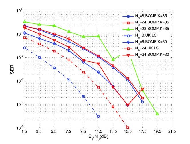
Figure 1: symbol recovery with 8 antennas at BS

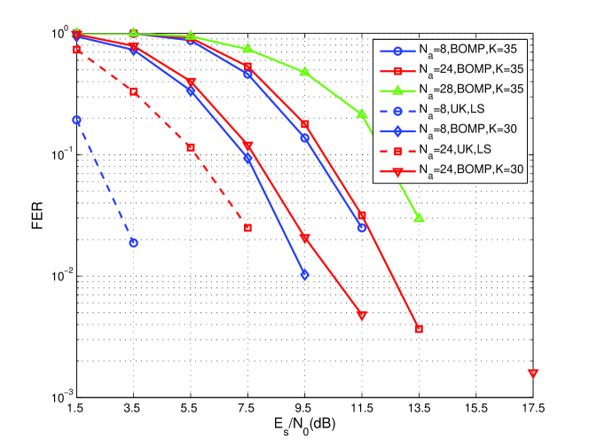
Figure 2: frame recovery with 8 antennas at BS

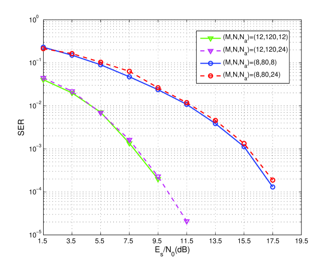
Figure 3: symbol recovery with different numbers of antennas at BS

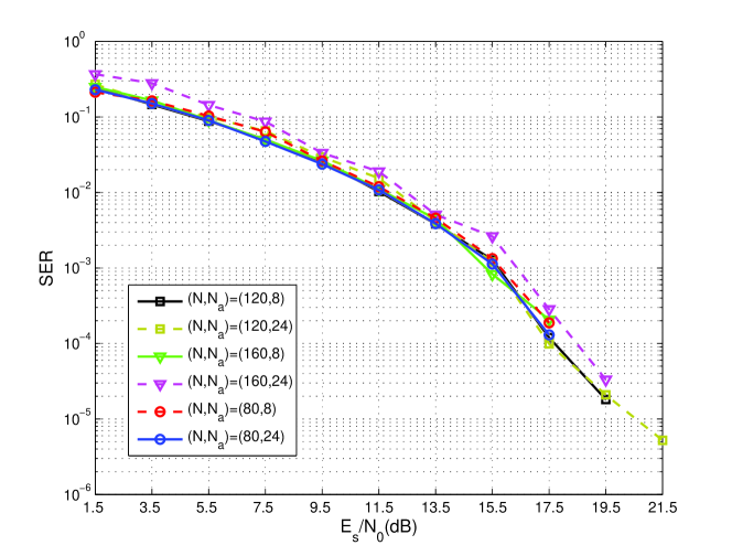
Figure 4: symbol recovery with different numbers of online users

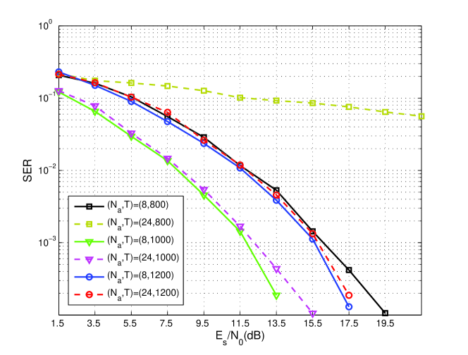
Figure 5: symbol recovery with different lengths of frames

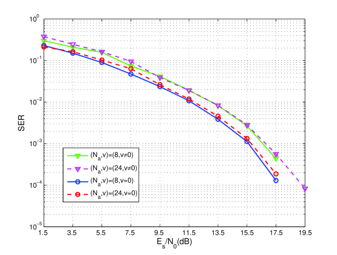
Figure 6: symbol recovery with or without column orthogonal blocks

In the first experiments, we have the simulations of BOMP algorithm to check the influences of different parameters. We assume that all the messages have the same length $d$, and we simply design ${\mathbf{P}}_{n}$ a random matrix with $(v=0)$ or without $(v\neq 0)$ orthogonal columns, $n=1,2,\ldots,N$.

In our simulation, the SER is computed as follows: when a demodulated signal of an active user is different from its original signal, we claim a symbol error; if an active user is not identified, then all $d$ symbol of that user are treated as erroneous.

Test Case 1: Figure 1 shows the performance of the proposed scheme with 8 antennas at BS, where $K$ is the number of iterations for BOMP algorithm. Other parameters are given as $(N,d,T,v)=(80,200,1000,0)$. The results indicate that, the SER increases when the number of active users becomes larger. For case where number of iterations is 35, when the number of active users is lower than a certain number, say 24 in our results, the SER is basically independent of the number of active users. Besides, we have observed that out of 35 iterations, in most cases the $N_{a}$ ($N_{a}<24$) active users can be successfully identified.

Also in Figure 1, we give results when less number of iterations is set for BOMP algorithm. When there are not too many active users, such as 8 users, fewer iterations are needed. But for 24 active users, 30 iterations are not enough to include all the active users. We also plotted two curves of reference in dotted lines. Both curves were obtained under the conditions that the actual active users are already known (users known, UK) and picked out. From the results, we can conclude that the number of non-active users has a great influence on the performance, even greater than that of active users.

Test Case 2: Corresponding to Figure 1 in SER, the FER is depicted Figure 2 with the same settings. In our simulation, the FER is computed as follows: when more than 8 bits in a message are demodulated in error, we claim a frame error. If the bit errors are equal to or less than 8, we hypothesize that they can be detected and corrected by the channel coding schemes. The same trend in FER performance can be observed as SER. When the $E_{s}/N_{0}$ exceeds a certain threshold, the FER will be negligible.

The normalized throughput is defined as $(1-P_{\text{FER}})N_{a}d/(MT)$, where $(1-P_{\text{FER}})N_{a}$ is the maximum number of allowed active users in our scheme, $P_{\text{FER}}$ is the value of FER; and $MT/d$ is the maximum number of users that can be served when all time slots of a frame are effectively used for data transmission, which is $40$ under the given parameters. If 24 active users are allowed to be simultaneously served, the throughput will reach 60% of maximum possible. In contrast, in conventional random access protocols, if we treat the signaling messages (such as request-to-send (RTS) signaling [4], [5]) also as small packets, the system throughput will be no more than 60%. Furthermore, if collision happens, which is often the case, the throughput will decrease a step further. Therefore, our scheme will greatly improve the system throughput compared to conventional schemes.

Test Case 3: In Figure 3, we compare the performance when BS are equipped with different numbers of antennas. Other parameters are given as $(d,T,K,v)=(200,1000,35,0)$. The results show that, when the number of antennas $M$ increases, the SER performance becomes remarkably better and a higher ratio $N_{a}/M$ can be accepted. On the other hand, a big performance gap between 8 antennas and 12 antennas at BS is observed. More antennas at BS allows a larger number of iterations for BOMP algorithm to accommodate more active users, and the big performance gap appears when we set both cases the same number 35 of iterations.

Test Case 4: From Figure 4 with parameters $(M,d,T,K,v)=(8,200,1000,35,0)$, we can see that when the number of active users is fixed, the SER increases as the number of online users increases, but the performance degradation is rather small, even when the number of online users has been doubled, nearly no more than 1dB degradation can be observed for 24 active users. By Theorem 3, the number of online users is not the dominant factor to affect the performance under the given parameters.

Test Case 5: Figure 5 depicts the performance when frame lengths are different, respectively for $T=4d$, $T=5d$ and $T=6d$. Other parameters are given as $(M,N,d,v)=(8,80,200,0)$. The number of iterations $K$ is set to 28, 35 and 42, respectively. The results show that the longer the frame length is, the better performance, and hence the more users that can be simultaneously served. However, affected by the normalization of columns in precoding matrix, even when the length of frame grows, the benefits diminish. This phenomenon will be observed when parameters are chosen to ensure that $MT/(dK)$ is a constant.

Test Case 6: In Figure 6, we investigate the effect of orthogonality of the block of the dictionary on the performance. Other parameters are given as $(M,N,d,T,K)=(8,80,200,1000,35)$. As we can see, for column non-orthogonal case, nearly 1dB performance degradation is observed when compared with that of column orthogonal condition.

TABLE I: Theoretical Analysis ($v=0$)

$M$	$N$	$d$	$T$	$\langle{{s_{l}}}\rangle(\langle{{s_{u}}}\rangle)$	$\beta$	$\mu_{{\mathbf{B}}}$	$\tau$	$N_{a.lowwer}(E_{s}/N_{0})$
								0dB	10dB	15dB
8	80	200	1000	$14.14$	2	$0.0035$	$15.00$	0	1	1
50	500	200	1000	$14.14$	2	$0.0019$	$15.00$	1	1	1
100	1000	200	1000	$14.14$	2	$0.0014$	$15.00$	1	2	2
8	80	200	1000	$14.14$	2	$0.0035$	$14.20$	0	1	1
50	500	200	1000	$14.14$	2	$0.0019$	$14.20$	1	1	1
100	1000	200	1000	$14.14$	2	$0.0014$	$14.20$	1	2	2
8	80	100	500	10	2	$0.0066$	$15.00$	0	1	1
50	500	100	500	10	2	$0.0037$	$15.00$	1	1	1
100	1000	100	500	10	2	$0.0030$	$15.00$	1	1	1

The results of our theoretical analysis of Theorem 1 for the case where $v=0$ and all messages have same length are shown in Table I, giving minimum number of active users that can be simultaneously served. Obviously, the bounded minimum number of active users is pessimistic when compared with our simulation results. At the same time, such pessimistic result can also be seen in the theoretical analysis for SER, for condition $1-(d-1)\nu-(K-1)d\mu_{\mathbf{B}}>0$ can not always be satisfied.

Remark 5: In all above simulations, we have set $d$ as the length of all messages. In practice, this may not be the case. In fact, when different lengths for messages exist and the number of active users is large, it has some slight performance degradation. For example, similar result can be observed when there are 24 active users and length of each message is uniformly distributed in the interval from 50 to 200. On the other hand, performance gap between $d=100$ and $d=200$ is barely visible.

V-B Performance Of ICBOMP Algorithm

In this part, we will apply ICBOMP algorithm to recover the transmitted signals.

Test Case 7: The results of FER for 8 antennas at BS are depicted in Figure 7, and other parameters are given as $(N,d,T,v)=(80,200,1000,0)$. For ICBOMP algorithm, we choose the channel coding scheme that is capable of correcting at most 8 bits for message of 200 symbols, e.g., a shortened BCH(472,400), which enjoys a relatively high code rate. When the error of a message is beyond correction, a frame error is declared.

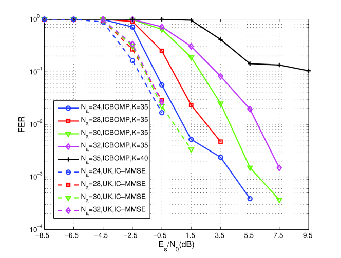
Figure 7: Frame recovery with 8 antennas at BS by ICBOMP algorithm

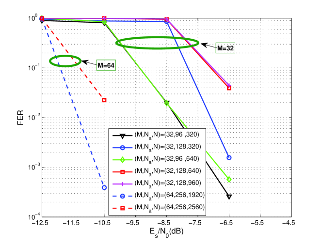
Figure 8: frame recovery with 32 and 64 antennas at BS by ICBOMP algorithm

Compared with Figure 1 achieved by BOMP algorithm, Figure 7 shows that ICBOMP algorithm can greatly improve the recovering performance, and more active users can be served simultaneously, say 30 or 32. Thus the throughput will be increased a step further, reaching 75% or 80% of the maximum possible. When ICBOMP algorithm is applied, the result we obtain for 24 active users with 35 iterations is almost identical to that achieved by 30 iterations, and we just depict one of them for clarity. Therefore, ICBOMP algorithm can also narrow the performance gap between different iteration numbers. It is also noticed that the performance gap between different numbers of active users have been widened.

Also, we included several curves in dotted lines to show the performance when actual active users are already picked out and no non-active users are chosen and interference-cancellation minimum mean-squared error (IC-MMSE) receiver is used. The IC-MMSE receiver performs iteratively MMSE decoding and perfect IC until more iterations no longer benefit. Perfect IC in IC-MMSE receiver is operated as in the ICBOMP algorithm. It shows that our ICBOMP receiver achieves a little worse performance than the IC-MMSE receiver, about 1dB performance degradation for 24 active users and 2dB performance degradation for 28 active users. Although for ICBOMP receiver, performance degradation exists when compared with IC-MMSE receiver, it is still highly competitive, since it requires no knowledge about active users. In fact, the ICBOMP receiver is able to achieve better performance than MMSE receiver when the number of active users is no more than 30.

Test Case 8: For massive MIMO, 8 or 12 antennas at BS are not enough. In the following, we present the FER performance with 32 and 64 antennas at BS in Figure 8, and other parameters are given as $(d,T,v)=(31,155,0)$. To ease the computational burden, we set the length for each message to 31. Channel coding scheme is assumed such that up to 1 bit of error can be corrected; e.g., a shortened BCH(69,62) could be used. When the number of errors in a message is larger than the designed error correction capability, a frame error is declared. The results show that, with more antennas, great improvements in performance are observed, and many more active users and online users can be accommodated.

VI Discussions

In this section, we discuss a few issues related to the design of our proposed scheme and its practical significance.

VI-A Dictionary Design

By Theorem 1, the smaller the block-coherence $\mu_{\mathbf{B}}$ and $\nu$ are, the better performance we can achieve, and thus the more active users the model can simultaneously accommodate. The authors in [19] had a discussion about the design of the dictionary that can lead to significant improvement in data recovery in block-sparse model. In our model, only the precoding matrix is up to our design.

In our scheme, when the number of active users is more than the number of antennas at BS, the channel vectors among users are correlated, even with massive MIMO technique. However, by our precoding scheme, correlations among columns in ${\mathbf{B}}$ can be smaller than correlations among channel vectors of different users, which means that block-coherence $\mu_{\mathbf{B}}$ can still be rather small, as long as precoding is well designed.

VI-B Application To Asynchronous Setting

Random MAC channel is usually asynchronous [22], while in our model, frame synchronization is assumed. In fact, our model can also be adjusted to quasi-synchronous setting, as long as the maximum asynchronism is known to the receiver. In such scenario, we can handle the problem by lengthening the maximum length $d$ with addition of the maximum asynchronous level, leading to a slight adjustment in the length of each precoding sequence. Readers can refer to [22] for more details.

VI-C Sparsity Level Selection

In our model, since we do not know exactly the number of active users a priori, a large number of iterations are usually needed for BOMP or ICBOMP algorithm. When there are not too many active users, however, unnecessary iterations increases computational cost. For example, our statistical results indicate that, when $E_{s}/N_{0}\geq 10$dB and with the same conditions for simulation of $8$ active users in Figure 1, 12 iterations for BOMP algorithm will correctly identify all the active users with a probability exceeding 99.9%. And for ICBOMP algorithm, even less iterations and higher probability can be anticipated. To address this problem, some methods for sparsity level selection will work, such as sparsity adaptive matching pursuit in [30]. When the number of active users is large, sparsity level identification may not bring too much benefit.

VI-D Message Segmentation

Messages of small packet can be segmented into shorter parts further, and each part can be transmitted with our scheme. When this method is adopted, we not only alleviate the computational complexity, but also ease the requirement for coherent time of channel. Besides, we can decrease the length uncertainty for each segmented part, and shorten the transmission duration for small packets whose lengths are short. More importantly, such approach may even be adopted to data transmission for messages that are not belonging to small packet.

VII Conclusion

In this paper, we proposed an uplink data transmission scheme for small packets. The proposed scheme combines the techniques of block precoding and sparsity-aware detection. It is especially suitable for system with a large number of antennas at the base station. Under the assumption that the BS has perfect CSI of every online user, we developed a block-sparse system model and adopted BOMP algorithm and its improved version ICBOMP algorithm to recover the transmitted data. With the ICBOMP algorithm which utilizes the function of error correction and detection coding to perform perfect IC in each iteration, an significant performance improvement was observed.

The transmission scheme considered in this paper is applicable to future wireless communication system. The reason is that small packets play a more and more important role in the data traffic due to the wide usage of intelligent terminals. The overall throughput of such a system is currently hampered by small packets because of the heavy signaling overhead. Our scheme will greatly reduce the signaling overhead and improve the throughput of such systems.

Appendix A Proof of Theorem 1

We first present a few results and lemmas that are useful for the proof of Theorem 1. Our proof of Theorem 1 follows along the lines of [20].

First of all, we present two useful results that have been obtained in some literature cites.

Result 1.

[20, Lemma 1] Given the dictionary ${\mathbf{B}}$ of normalized columns with block-coherence $\mu_{\mathbf{B}}$ and sub-coherence $\nu$, it holds that

$$\max_{i\neq j}\|{\mathbf{B}}_{i}^{H}{\mathbf{B}}_{j}\|\leq d\mu_{\mathbf{B}}$$ (31)

and

$$1-(d-1)\nu\leq\|{\mathbf{B}}_{i}^{H}{\mathbf{B}}_{i}\|\leq 1+(d-1)\nu$$ (32)

Provided that $1-(d-1)\nu-(K-1)d\mu_{\mathbf{B}}>0$ and $|I|\leq K$, it holds that

$$\|({\mathbf{B}}_{I}^{H}{\mathbf{B}}_{I})^{-1}\|\leq[1-(d-1)\nu-(K-1)d\mu_{\mathbf{B}}]^{-1}$$ (33)

Result 2.

[29, §10.2] Denote $m\times n$ matrices ${\mathbf{A}}$ and ${\mathbf{C}}$, whose singular values are $\sigma_{1}\geq\ldots\geq\sigma_{n}$, $\gamma_{1}\geq\ldots\geq\gamma_{n}$, respectively, then

$$-\sum_{i=1}^{n}\sigma_{i}\gamma_{i}\leq\text{Re}[\text{Tr}({\mathbf{A}}{\mathbf{C}}^{H})]\leq\sum_{i=1}^{n}\sigma_{i}\gamma_{i}$$ (34)

In the following, two lemmas will be given.

Lemma 1.

Consider the block-sparse model in model (4) and the condition $\tau=\max_{1\leq j\leq N}\|{\mathbf{B}}_{j}^{H}{\mathbf{z}}\|_{2}$. Provided that

$$\begin{split}\rho_{0}M[1-(d-1)\nu]^{2}s_{u}^{2}&>\tau^{2}+\rho_{0}M(d\mu_{\mathbf{B}})^{2}N_{a}^{2}s_{u}^{2}+2\rho_{0}Md\mu_{\mathbf{B}}\{(N_{a}-1)[1+(d-1)\nu]\}s_{l}^{2}\\ &\quad+2\sqrt{\rho_{0}M}\tau\{(N_{a}-1)d\mu_{\mathbf{B}}+[1+(d-1)\nu]\}s_{l}+2\sqrt{\rho_{0}M}N_{a}d\mu_{\mathbf{B}}\tau s_{u}\end{split}$$ (35)

it holds that

$$\max_{j\in I}\|{\mathbf{B}}_{j}^{H}{\mathbf{y}}\|_{2}>\max_{j\notin I}\|{\mathbf{B}}_{j}^{H}{\mathbf{y}}\|_{2}$$ (36)

Proof:

Note that

$$\begin{split}\|{\mathbf{B}}_{j}^{H}{\mathbf{y}}\|_{2}^{2}&={\mathbf{y}}^{H}{\mathbf{B}}_{j}{\mathbf{B}}_{j}^{H}{\mathbf{y}}\\ &=\text{Tr}\{{\mathbf{B}}_{j}^{H}{\mathbf{y}}{\mathbf{y}}^{H}{\mathbf{B}}_{j}\}\\ &=\text{Tr}\left\{{\mathbf{B}}_{j}^{H}\left[\sqrt{\rho_{0}M}(\sum_{i\in I}{\mathbf{B}}_{i}{\mathbf{s}}_{i})+{\mathbf{z}}\right]\left[\sqrt{\rho_{0}M}(\sum_{i\in I}{\mathbf{B}}_{i}{\mathbf{s}}_{i})+{\mathbf{z}}\right]^{H}{\mathbf{B}}_{j}\right\}\end{split}$$ (37)

Then we have

$$\begin{split}\max_{j\notin I}\|{\mathbf{B}}_{j}^{H}{\mathbf{y}}\|_{2}^{2}&=\max_{j\notin I}\text{Tr}\left({\mathbf{B}}_{j}^{H}{\mathbf{y}}{\mathbf{y}}^{H}{\mathbf{B}}_{j}\right)\\ &=\max_{j\notin I}\rho_{0}M\cdot\text{Tr}\left[(\sum_{i\in I}{\mathbf{B}}_{j}^{H}{\mathbf{B}}_{i}{\mathbf{s}}_{i})(\sum_{i\in I}{\mathbf{s}}_{i}^{H}{{\mathbf{B}}_{i}^{H}}{\mathbf{B}}_{j})\right]\\ &\quad+\max_{j\notin I}2\sqrt{\rho_{0}M}\cdot\text{Re}\left\{\text{Tr}\left[(\sum_{i\in I}{\mathbf{B}}_{j}^{H}{\mathbf{B}}_{i}{\mathbf{s}}_{i}){\mathbf{z}}^{H}{\mathbf{B}}_{j}\right]\right\}+\max_{j\notin I}\text{Tr}\left({\mathbf{B}}_{j}^{H}{\mathbf{z}}{\mathbf{z}}^{H}{\mathbf{B}}\right)\end{split}$$ (38)

Note that for vectors ${\tilde{\mathbf{x}}}\in\mathbb{C}^{n\times 1}$ and ${\tilde{\mathbf{y}}}\in\mathbb{C}^{n\times 1}$, the matrix ${\tilde{\mathbf{x}}}{\tilde{\mathbf{y}}}^{H}$ at most has one nonzero singular value which equals to the absolute value of ${\tilde{\mathbf{x}}}^{H}{\tilde{\mathbf{y}}}$. In addition, for any matrix ${\mathbf{A}}\in\mathbb{C}^{n\times n}$, matrix ${\tilde{\mathbf{x}}}{\tilde{\mathbf{y}}}^{H}{\mathbf{A}}$ also has at most one nonzero singular value which equals to the absolute value of ${\tilde{\mathbf{x}}}^{H}{\mathbf{A}}^{H}{\tilde{\mathbf{y}}}$, and it holds that $\|{\tilde{\mathbf{x}}}{\tilde{\mathbf{y}}}^{H}{\mathbf{A}}\|=|{\tilde{\mathbf{x}}}^{H}{\mathbf{A}}^{H}{\tilde{\mathbf{y}}}|=|({\tilde{\mathbf{x}}},{\mathbf{A}}^{H}{\tilde{\mathbf{y}}})|\leq\|{\tilde{\mathbf{x}}}\|_{2}\|{\mathbf{A}}^{H}{\tilde{\mathbf{y}}}\|_{2}\leq\|{\mathbf{A}}\|\|{\tilde{\mathbf{x}}}\|_{2}\|{\tilde{\mathbf{y}}}\|_{2}$. Together with Result 1 and Result 2, we have

$$\max_{j\notin I} \text{Tr}\{(\sum_{i\in I}{\mathbf{B}}_{j}^{H}{\mathbf{B}}_{i}{\mathbf{s}}_{i})(\sum_{i\in I}{\mathbf{s}}_{i}^{H}{\mathbf{B}}_{i}^{H}{\mathbf{B}}_{j})\}$$ (39)

$$\leq N_{a}\{\max_{i\neq j}\text{Tr}\{({\mathbf{B}}_{j}^{H}{\mathbf{B}}_{i})({\mathbf{s}}_{i}{\mathbf{s}}_{i}^{H}{\mathbf{B}}_{i}^{H}{\mathbf{B}}_{j})\}\}+(N_{a}^{2}-N_{a})\{\max_{i\neq j\neq r}\text{Tr}\{({\mathbf{B}}_{j}^{H}{\mathbf{B}}_{i})({\mathbf{s}}_{i}{\mathbf{s}}_{r}^{H}{\mathbf{B}}_{r}^{H}{\mathbf{B}}_{j})\}\}$$

$$\leq N_{a}\{\max_{i\neq j}\|{\mathbf{B}}_{j}^{H}{\mathbf{B}}_{i}\|\|{\mathbf{s}}_{i}{\mathbf{s}}_{i}^{H}{\mathbf{B}}_{i}^{H}{\mathbf{B}}_{j}\|\}+(N_{a}^{2}-N_{a})\{\max_{i\neq j\neq r}\|{\mathbf{B}}_{j}^{H}{\mathbf{B}}_{i}\|\|{\mathbf{s}}_{i}{\mathbf{s}}_{r}^{H}{\mathbf{B}}_{r}^{H}{\mathbf{B}}_{j}\|\}$$ (40)

$$\leq N_{a}\{d\mu_{\mathbf{B}}d\mu_{\mathbf{B}}s_{u}^{2}\}+(N_{a}^{2}-N_{a})\{d{\mu_{\mathbf{B}}}d\mu_{\mathbf{B}}s_{u}^{2}\}$$ (41)

$$=N_{a}^{2}(d\mu_{\mathbf{B}})^{2}s_{u}^{2}$$ (42)

where we have used the identity $\text{Re}[\text{Tr}({\mathbf{A}}{\mathbf{A}}^{H})]=\text{Tr}({\mathbf{A}}{\mathbf{A}}^{H})$. Furthermore, we have

$$\max_{j\notin I}\text{Re}\left\{\text{Tr}\left[(\sum_{i\in I}{\mathbf{B}}_{j}^{H}{\mathbf{B}}_{i}{\mathbf{s}}_{i}){\mathbf{z}}^{H}{\mathbf{B}}_{j}\right]\right\} \leq N_{a}\max_{i\neq j}\text{Re}[\text{Tr}({\mathbf{B}}_{j}^{H}{\mathbf{B}}_{i}{\mathbf{s}}_{i}{\mathbf{z}}^{H}{\mathbf{B}}_{j})]$$ (43)

$$\leq N_{a}\max_{i\neq j}\|{\mathbf{B}}_{j}^{H}{\mathbf{B}}_{i}\|\|{\mathbf{s}}_{i}{\mathbf{z}}^{H}{\mathbf{B}}_{j}\|$$ (44)

$$=N_{a}d\mu_{\mathbf{B}}\tau s_{u}$$ (45)

By the definition of $\tau$

$$\max_{j\notin I}\text{Tr}\{{\mathbf{B}}_{j}^{H}{\mathbf{z}}{\mathbf{z}}^{H}{\mathbf{B}}_{j}\}=\max_{j\notin I}\|{\mathbf{B}}_{j}^{H}{\mathbf{z}}\|_{2}^{2}\leq\tau^{2}$$ (46)

From derivations above, we obtain

$$\max_{j\notin I}\|{\mathbf{B}}_{j}^{H}{\mathbf{y}}\|_{2}^{2}\leq\rho_{0}MN_{a}^{2}(d\mu_{\mathbf{B}})^{2}s_{u}^{2}+2\sqrt{\rho_{0}M}N_{a}d\mu_{\mathbf{B}}\tau s_{u}+\tau^{2}$$ (47)

On the other hand, we have

$$\max_{j\in I}\text{Tr}\{(\sum_{i\in I}{\mathbf{B}}_{j}^{H}{\mathbf{B}}_{i}{\mathbf{s}}_{i})(\sum_{i\in I}{\mathbf{s}}_{i}^{H}{\mathbf{B}}_{i}^{H}{\mathbf{B}}_{j})\} =\max_{j\in I}\text{Tr}\{{\mathbf{B}}_{j}^{H}{\mathbf{B}}_{j}{\mathbf{s}}_{j}{\mathbf{s}}_{j}^{H}{\mathbf{B}}_{j}^{H}{\mathbf{B}}_{j}\}$$ (48)

$$\quad+\max_{j\in I}2\text{Re}\{\text{Tr}\{({\mathbf{B}}_{j}^{H}{\mathbf{B}}_{j}{\mathbf{s}}_{j})(\sum_{i\in I\backslash\{j\}}{\mathbf{s}}_{i}^{H}{{\mathbf{B}}_{i}^{H}}{\mathbf{B}}_{j})\}\}$$ (49)

$$\quad+\max_{j\in I}\text{Tr}\{(\sum_{i\in I\backslash\{j\}}{\mathbf{B}}_{j}^{H}{\mathbf{B}}_{i}{\mathbf{s}}_{i})(\sum_{i\in I\backslash\{j\}}{\mathbf{s}}_{i}^{H}{\mathbf{B}}_{i}^{H}{\mathbf{B}}_{j})\}$$ (50)

For each summation term above, the first term

$$\max_{j\in I}\text{Tr}\{{\mathbf{B}}_{j}^{H}{\mathbf{B}}_{j}{\mathbf{s}}_{j}{\mathbf{s}}_{j}^{H}{\mathbf{B}}_{j}^{H}{\mathbf{B}}_{j}\} =\max_{j\in I}\{{\mathbf{s}}_{j}^{H}({\mathbf{B}}_{j}^{H}{\mathbf{B}}_{j})^{2}{\mathbf{s}}_{j}\}$$ (51)

$$\geq\lambda_{\min}\{({\mathbf{B}}_{j}^{H}{\mathbf{B}}_{j})^{2}\}\max_{j\in I}\{\|{\mathbf{s}}_{j}{\mathbf{s}}_{j}^{H}\|\}$$ (52)

$$=[1-(d-1)\nu]^{2}s_{u}^{2}$$ (53)

in which Gershgorin circle theorem and Rayleigh-Ritz theorem have been used. By Gershgorin circle theorem and the property of eigenvalue, all the eigenvalues of $({\mathbf{B}}_{j}^{H}{\mathbf{B}}_{j})^{2}$ are in the range
$[(1-(d-1)\nu)^{2},(1+(d-1)\nu)^{2}]$. At the same time, just like the derivation when $j\notin I$, the second summation term can be bounded as

$$\max_{j\in I}2\text{Re}\{\text{Tr}\{({\mathbf{B}}_{j}^{H}{\mathbf{B}}_{j}{\mathbf{s}}_{j})(\sum_{i\in I\backslash\{j\}}{\mathbf{s}}_{i}^{H}{\mathbf{B}}_{i}^{H}{\mathbf{B}}_{j})\}\}\geq-2(N_{a}-1)[1+(d-1)\nu]d\mu_{\mathbf{B}}s_{l}^{2}$$ (54)

And for the third term

$$\max_{j\in I}\text{Tr}\{(\sum_{i\in I\backslash\{j\}}{\mathbf{B}}_{j}^{H}{\mathbf{B}}_{i}{\mathbf{s}}_{i})(\sum_{i\in I\backslash\{j\}}{\mathbf{s}}_{i}^{H}{\mathbf{B}}_{i}^{H}{\mathbf{B}}_{j})\}\geq 0$$ (55)

Besides, since

$$\max_{j\in I} \text{Re}\{\text{Tr}\{(\sum_{i\in I}{\mathbf{B}}_{j}^{H}{\mathbf{B}}_{i}{\mathbf{s}}_{i}){\mathbf{z}}^{H}{\mathbf{B}}_{j}\}\}$$ (56)

$$=\max_{j\in I}\text{Re}\{\text{Tr}\{\sum_{i\in I\backslash\{j\}}{\mathbf{B}}_{j}^{H}{\mathbf{B}}_{i}{\mathbf{s}}_{i}{\mathbf{z}}^{H}{\mathbf{B}}_{j}+{\mathbf{B}}_{j}^{H}{\mathbf{B}}_{j}{\mathbf{s}}_{j}{\mathbf{z}}^{H}{\mathbf{B}}_{j}\}\}$$ (57)

$$\geq-(N_{a}-1)d\mu_{\mathbf{B}}\tau s_{l}-[1+(d-1)\nu]\tau s_{l}$$ (58)

and

$$\max_{j\in I} \text{Tr}\{{\mathbf{B}}_{j}^{H}{\mathbf{z}}{\mathbf{z}}^{H}{\mathbf{B}}_{j}\}\geq 0$$ (59)

we have

$$\max_{j\in I}\|{\mathbf{B}}_{j}^{H}{\mathbf{y}}\|_{2}^{2} \geq\rho_{0}M[1-(d-1)\nu]^{2}s_{u}^{2}-2\rho_{0}M(N_{a}-1)[1+(d-1)\nu]d\mu_{\mathbf{B}}s_{l}^{2}$$ (60)

$$\quad-2\sqrt{\rho_{0}M}\tau[(N_{a}-1)d\mu_{\mathbf{B}}+[1+(d-1)\nu]]s_{l}$$ (61)

Then we have

$$\max_{j\in I}\|{\mathbf{B}}_{j}^{H}{\mathbf{y}}\|_{2}^{2}-\max_{j\notin I}\|{\mathbf{B}}_{j}^{H}{\mathbf{y}}\|_{2}^{2} \geq\rho_{0}M[1-(d-1)\nu]^{2}s_{u}^{2}-\tau^{2}-2\sqrt{\rho_{0}M}N_{a}d\mu_{\mathbf{B}}\tau s_{u}$$ (62)

$$\quad-\rho_{0}Md\mu_{\mathbf{B}}\{2(N_{a}-1)[1+(d-1)\nu]s_{l}^{2}+N_{a}^{2}d\mu_{\mathbf{B}}s_{u}^{2}\}$$ (63)

$$\quad-2\sqrt{\rho_{0}M}\tau\{(N_{a}-1)d\mu_{\mathbf{B}}+[1+(d-1)\nu]\}s_{l}$$ (64)

By (62), Lemma 1 is proved. ∎

Lemma 2.

Suppose ${\mathbf{u}}$ is a $MT$-dimensional circular symmetric Gaussian random vector of zero mean and ${\mathbf{I}}_{MT}$ covariance matrix, then

$$P\{{\tilde{\tau}}\geq\|{\mathbf{B}}_{j}^{H}{\mathbf{u}}\|_{2}\}\geq 1-e^{-\varsigma^{2}}\sum_{k=0}^{d-1}\frac{({{\varsigma^{2}}})^{k}}{k!}$$ (65)

where $\varsigma={\tilde{\tau}}/\sqrt{1+({d-1})\nu}$.

Proof:

Suppose vector ${\tilde{\mathbf{u}}}=\sqrt{2}{\mathbf{u}}$, then ${\tilde{\mathbf{u}}}$ satisfies the distribution of $\mathcal{CN}(0,2{\mathbf{I}})$. By [27], $\|{\tilde{\mathbf{u}}}\|_{2}^{2}$ is a chi-squared random variable with $2d$ degrees of freedom, then probability

$$Pr\{\|{\mathbf{u}}\|_{2}^{2}\geq t^{2}\}=Pr\{\|{\tilde{\mathbf{u}}}\|_{2}^{2}\geq 2t^{2}\}=\frac{\Gamma(d,t^{2})}{\Gamma(d)}$$ (66)

where series expansion of $\Gamma(a,z)$ in [28] gives that

$$\Gamma(d,t^{2})=\frac{e^{-t^{2}}}{2}t^{2}[(\sqrt{2}t)^{2d}+(2d-2)(\sqrt{2}t)^{2d-2}+\cdots+(2d-2)!!(\sqrt{2}t)^{2}]$$ (67)

By using the double factorial notation: $n!!=\prod_{0\leq i\leq\lfloor n/2\rfloor}{({n-2i})}$, and $\Gamma(d)=(d-1)!$, we will obtain

$$\frac{\Gamma(d,t^{2})}{\Gamma(d)} =e^{-t^{2}}[\frac{(t^{2})^{d-1}}{(d-1)!}+\frac{(t^{2})^{d-2}}{(d-2)!}+\frac{(t^{2})^{d-3}}{(d-3)!}+\cdots+\frac{(t^{2})^{0}}{0!}]$$ (68)

$$=e^{-t^{2}}\sum_{k=0}^{d-1}\frac{(t^{2})^{k}}{k!}$$ (69)

which yields the lemma.

Consider the event ${\tilde{\tau}}\geq\|{\mathbf{B}}_{j}^{H}{\mathbf{z}}\|_{2}$, as in [20], ${\mathbf{B}}_{j}^{H}{\mathbf{z}}$ is a $d$-dimensional Gaussian random vector with zero mean and ${\mathbf{B}}_{j}^{H}{\mathbf{B}}_{j}$ covariance matrix. Therefore, vector ${\mathbf{u}}=({\mathbf{B}}_{j}^{H}{\mathbf{B}}_{j})^{-1/2}{{\mathbf{B}}_{j}^{H}}{\mathbf{z}}$ is also a $d$-dimensional circular symmetric Gaussian random vector of mean zero and covariance ${\mathbf{I}}_{d}$. Then by Lemma 2 and Result 1 it is easy to demonstrate that

$$\Pr\{\|{\mathbf{B}}_{j}^{H}{\mathbf{z}}\|_{2}^{2}\leq{\tilde{\tau}}^{2}\} =\Pr\{\|({\mathbf{B}}_{j}^{H}{\mathbf{B}}_{j})^{1/2}{\mathbf{u}}\|_{2}^{2}\leq{\tilde{\tau}}^{2}\}$$ (70)

$$\geq\Pr\{\|({\mathbf{B}}_{j}^{H}{\mathbf{B}}_{j})\|\cdot\|{\mathbf{u}}\|_{2}^{2}\leq{\tilde{\tau}}^{2}\}$$ (71)

$$\geq\Pr\{\|{\mathbf{u}}\|_{2}^{2}\leq\frac{{\tilde{\tau}}^{2}}{1+(d-1)\nu}\}$$ (72)

$$=1-e^{-\varsigma^{2}}\sum_{k=0}^{d-1}\frac{(\varsigma^{2})^{k}}{k!}$$ (73)

where $\varsigma={\tilde{\tau}}/\sqrt{1+(d-1)\nu}$. ∎

With lemmas given above, we can prove Theorem 1 next.

Proof:

By the same induction in proof of [20, Theorem 5], when (13) is satisfied which verifies (35), for each iteration of BOMP, an most likely active user will be selected. Therefore, the actual support of the nonzero blocks can be correctly confirmed. Gathering all these $K$ selected blocks to form a set, say ${\hat{I}}$, we have $|{\hat{I}}|=K$, and $I\subseteq{\hat{I}}$, then

$$\|{\hat{\mathbf{s}}}_{BOMP}-{\mathbf{s}}\|_{2}^{2} =\|(\sqrt{\rho_{0}M}{\mathbf{B}}_{{\hat{I}}})^{\dagger}{\mathbf{y}}-{\mathbf{s}}\|_{2}^{2}$$ (74)

$$=\|(\sqrt{\rho_{0}M}{\mathbf{B}}_{{\hat{I}}})^{\dagger}{\mathbf{z}}\|_{2}^{2}$$ (75)

$$\leq(\rho_{0}M)^{-1}\|({\mathbf{B}}_{{\hat{I}}}^{H}{\mathbf{B}}_{{\hat{I}}})^{-1}\|^{2}\sum_{j\in{\hat{I}}}\|{\mathbf{B}}_{j}^{H}{\mathbf{z}}\|_{2}^{2}$$ (76)

$$\leq\frac{K\tau^{2}}{[1-(d-1)\nu-(K-1)d\mu_{\mathbf{B}}]^{2}\rho_{0}M}$$ (77)

where $\tau=\max_{1\leq j\leq N}\|{\mathbf{B}}_{j}^{H}{\mathbf{z}}\|_{2}$ and (33) in Result 1 are used. The theorem is thus established. ∎

References

- [1] R. E. Grinter and L. Palen, “Instant messaging in teen life,” in Proceedings of the ACM conference on Computer supported cooperative work, pp. 21-30, 2002.
- [2] Z. Xiao, L. Guo, and J. Tracey, “Understanding Instant Messaging Traffic Characteristics,” in Distributed Computing Systems, IEEE International Conference on, pp. 51-51, 2007.
- [3] X. He, P.P.C. Lee, L. Pan, et. al., “A panoramic view of 3G data/control-plane traffic: mobile device perspective.” NETWORKING 2012, Springer Berlin Heidelberg, pp. 318-330, 2012.
- [4] M. Park, R. Heath Jr., and S. M. Nettles, “Improving throughput and fairness for MIMO ad hoc networks using antenna selection diversity,” IEEE Global Telecommunications Conference, vol. 5, pp. 3363-3367, 2004.
- [5] C.K. Pan, Y. M. Cai, and Y.Y. Xu, “Channel-aware multi-user uplink transmission scheme for SIMO-OFDM systems,” Science in China Series F: Information Sciences, vol. 52, no. 9, pp. 1678-1687, 2009.
- [6] R. Xie, H. Yin, Z. Wang and X. Chen, “A Novel Uplink Data Transmission Scheme For Small Packets In Massive MIMO System,” to appear at IEEE/CIC 2014 Symposium on Signal Processing for Communications (ICCC).
- [7] E. G. Larsson, F. Tufvesson, O. Edfors, and T. L. Marzetta, “Massive MIMO for next generation wireless systems,” IEEE Communications Magazine, Feb. 2014.
- [8] F. Rusek, D. Persson, B. K. Lau, E. G. Larsson, T. L. Marzetta, O. Edfors, and F. Tufvesson, “Scaling up MIMO: Opportunities and challenges with very large arrays,” IEEE Signal Process. Mag., vol. 30, no. 1, pp. 40-60, 2013.
- [9] T. L. Marzetta, “Noncooperative cellular wireless with unlimited numbers of base station antennas,” IEEE Transactions on Wireless Communications, vol. 9, no. 11, pp. 3590-3600, 2010.
- [10] H. Ngo, E. Larsson, and T. Marzetta, “Energy and spectral efficiency of very large multiuser MIMO systems,” IEEE Transactions on Communications, vol. 61, no. 4, pp. 1436-1449, 2013.
- [11] D. Donoho, “Compressed Sensing,” IEEE Trans. Inform. Theory, vol. 52, no. 4, pp. 1289-1306, 2006.
- [12] E. J. Candés, J. Romberg, and T. Tao, “Robust Uncertainty Principles: Exact Signal Reconstruction from Highly Incomplete Frequency Information,” IEEE Trans. Inform. Theory, vol. 52, no. 2, pp. 489-509, 2006.
- [13] R. G. Baraniuk, “Compressive sensing,” IEEE Signal Process. Mag.,vol. 24, no. 4, pp. 118-120, 2007.
- [14] E. J. Candés and M. B. Wakin, “An introduction to compressive sampling,” IEEE Signal Process. Mag., vol. 25, no. 2, pp. 21-30, 2008.
- [15] M. F. Duarte and Y. C. Eldar, “Structured Compressed sensing: From Theory to Applications,” IEEE Trans. Signal Process., vol. 59, no. 9, pp. 4053-4085, 2011.
- [16] Y. Li, J. H. Winters, and N. T. Sollenberger, “MIMO-OFDM for Wireless Communications: Signal Detection with Enhanced Channel Estimation,” IEEE Transactions on Communications, vol. 50, no. 9, pp. 1471-1477, 2002.
- [17] P. Patel and J. Holtzman, “Performance comparison of a DS/CDMA system using a successive interference cancellation (IC) scheme and a parallel IC scheme under fading,” IEEE International Conference on Communications, pp. 510-514, 1994.
- [18] E. Biglieri, A. Nordio and G. Taricco, “MIMO Doubly-Iterative Receivers: Pre- vs. Post-Cancellation Filtering,” IEEE Commun. Lett, vol. 9, no. 2, pp. 106-108, 2005.
- [19] Y. C. Eldar, P. Kuppinger, and H. Bölcskei, “Block-sparse signals: Uncertainty relations and efficient recovery,” IEEE Trans. Signal Process., vol. 58, no. 6, pp. 3042-3054, 2010.
- [20] Z. B. Haim and Y. C. Eldar, “Near-Oracle Performance of Greedy Block-Sparse Estimation Techniques From Noisy Measurements,” IEEE Journal of Selected Topics in Signal Processing, vol. 5, no. 5, pp.1032-1047, 2011.
- [21] R. G. Baraniuk, V. Cevher, M. F. Duarte, and C. Hegde, “Model-based compressive sensing,” IEEE Trans. Inform. Theory, vol. 56, no. 4, pp.1982-2001, 2010.
- [22] L. Applebaum, W.U. Bajwa, M.F. Duarte, and R. Calderbank, “Asynchronous code-division random access using convex optimization,” Physical Communication, vol. 5, no. 2, pp. 129–147, 2012.
- [23] H. Li, R. Mao, L. Lai, and R. C. Qiu, “Compressed meter reading for delay-sensitive and secure load report in smart grid,” in IEEE Int. Conf. on Smart Grid Commun, pp. 114-119, 2010.
- [24] R. H. Y. Louie, W. Hardjawana, Y. Li and B. Vucetic, “Distributed Multiple-Access for Wireless Communications: Compressed Sensing with Multiple Antennas,” IEEE Globecom, pp. 3622-3627, 2012.
- [25] J. Luo and D. Guo, “Neighbor Discovery in Wireless Networks Using Compressed Sensing with Reed-Muller Codes,” in IEEE International Symposium on Modeling and Optimization in Mobile, Ad Hoc and Wireless Networks (WiOpt), pp. 154-160, 2011.
- [26] P. Viswanath and D. Tse, “Sum Capacity of the Vector Gaussian Broadcast Channel and Uplink-Downlink Duality,” IEEE Trans. Inform. Theory, vol. 49, no. 8, pp. 1912-1921, 2003.
- [27] A. Stuart and J. K. Ord, Kendall’s Advanced Theory of Statistics, 6nd edition, London, U.K.: Edward Arnold, vol. 1, 1994.
- [28] M. Abramowitz and I. A. Stegun, Handbook of Mathematical Functions With Formulas, Graphs, and Mathematical Tables, New York, Dover, 1964.
- [29] J. Kuang, Applied Inequalities, 4nd edition, Hunan Education Press, Changsha, China, 1993.
- [30] T. T. Do, L. Gan, N. Nguyen, and T. D. Tran, “Sparsity adaptive matching pursuit algorithm for practical compressed sensing,” in 42nd Asilomar Conf. on Signals, Systems and Computers, pp. 581-587, 2008.
- [31] T. M. Cover and J. A. Thomas, Elements of Information Theory. New York: Wiley, 2006.