Charged star in (2+1)-dimensional gravity

Abstract

We obtain a new class of exact solutions for the Einstein-Maxwell system in static spherically symmetric charged star in (2+1)-dimensional gravity. In order to obtain the analytical solutions we treat the matter distribution anisotropic in nature admitting linear or nonlinear equation of state and the electric field intensity was specified. By choosing a suitable choice of mass function m(r), it is possible to integrate the system in closed form. All the solution, which are obtained in both linear and nonlinear cases are regular at the center and well behaved in the stellar interior.

I Introduction

For finding the comprehensive picture of today’s universe, researchers are trying to solve Einstein’s equation with different inputs for physical contact (dust, perfect fluid, etc.) and feature (charge, rotation, anisotropic matter, etc.). In relativistic astrophysics, the study of static anisotropic fluid spheres attracts the interest of researchers after the extensive investigation by Bowers and Liagn Bowers and Liang (1995), and the theoretical investigations by R. Ruderman Ruderman (1995), showing that the nuclear matter may be anisotropic (i.e. radial pressure may not be equal to the tangential pressure) in a very high density range ($\rho>10^{15}$ $g/cm^{3}$) where nuclear interaction need to be treated relativistically. A large number of study have been found corresponding to the anisotropic matter applied to the relativistic star when the gravitational field is taken to be static spherically symmetric which is commonly done by matching two given and known space-time at the junction surface.

In recent year, lower dimensional gravity has turn into a special attention for its simplicity to describe the geometry of space-time. Specially it enlighten some ambiguity which appeared in four dimensional gravity. For example, the study of black hole become more complicated in four dimensional gravity. To overcome these difficulties and get reasonable acceptable results, researchers have resorted to the models in the lower dimensional gravity. On this respect most revolutionary work had been done by Bañados, Teitelboim and Zanelli Ba$\tilde{n}$ados et al (1992), with the discovery of (2+1) dimensional black hole with negative cosmological constant known as BTZ black hole which has many similarity with the characteristic of four dimensional black hole. The interesting features of BTZ black holes are, it is a solution of low energy string theory with a non-vanishing antisymmetric tensor and it can be matched to the exterior of a (2+1) dimensional perfect fluid star. With this point of view Cruz and Zanelli Cruz and Zanelli (1995), studied the stability of these stars and puts an upper limit for mass considering generic equation of state $P=P(\rho)$. Garcí a and Campuzano Garcí a and Campuzano (2003), have derived all static circularly symmetric perfect fluid 2+1 dimensional gravity and made an important conclusion that by a simple dimensional reduction one can get a 2+1 perfect fluid solution with constant energy density that can be derived from the Schwarzschild interior metric by a comparison with (2+1) and (3+1) gravity. Mann and Ross Mann and Ross (1993), shown that a (2+1) dimensional star filled with dust (P=0), might collapsed to a black hole under certain conditions. David Garfinkel D. Garfinkle (2003), have found an exact solution for the critical collapse of a scalar field in closed form for (2+1) dimensional gravity with negative cosmological constant. Another interesting solution have found by Paulo M. Sá Paulo M. S$\acute{a}$ (1999) for three-dimensional perfect fluid stars with polytropic equation of state of the form $P=K\rho^{1+\frac{1}{n}}$, where ‘n’ is polytropic index and K is polytropic constant. Recently, Sharma et al Sharma et al (2011) have found a star solution with simple analytical form by choosing the form of the mass function m(r). Motivated by the work we have found a new star solution, assuming the interior space-time is Finch-skea type for (2+1) dimensions and match the exterior with anti-de Sitter BTZ metric in Banerjee et al (2013).

Our objective is to find a new solutions of the Einstein-Maxwell system satisfying the necessary criteria of a neutral star solution in (2+1)-dimensional gravity. A spherically symmetric charged ideal fluid solution of Einstein field equation has been studied by N. $\ddot{O}$zdemir N. Ozdemiret al (2007) in the presence of the cosmological constant. Mak and Harko M. K. Maket al (1989) obtained an exact analytical solution for describing the interior of a charged strange quark star under the assumption of spherical symmetry and the existence of a one-parameter group of conformal motions. A well studied of charged objects in the frame of General Relativity, by solving the coupled Einstein-Maxwell field equations has been found in K. Komathirajet al (2007); R.Sharmaet al (2001); L.K. Patelet al (1987, 1997); S.Thirukkaneshet al (1997). Varela et al V. Varelaet al (2010) have found an analytical solutions for self-gravitating, charged, anisotropic fluids with linear or non-linear equations of state and obtain more flexibility in solving the Einstein-Maxwell equations.

In this paper, we discuss a new type of charged star in (2+1) dimensional gravity assuming the matter distribution is anisotropic in nature admitting a linear or nonlinear EOS. We match our interior solutions corresponding to the exterior charged BTZ metric with zero spin. The solution which we obtained, satisfied all the regularity conditions for a star solution and its simple analytic form helps to evaluate the physical parameters in a simple manner for the star solution.

II Field equations and Interior geometry

We assume that the gravitational field should be static and spherically symmetric for describing the internal geometry of a charged relativistic compact object. For describing such a configuration in (2+1)-dimensional gravity the line element is given by

$$ds^{2}=-e^{\nu(r)}dt^{2}+e^{\mu(r)}dr^{2}+r^{2}d\theta^{2},$$ (1)

where $\nu(r)$ and $\mu(r)$ are the two unknown metric functions. Following an earlier treatment Rahaman et al (2012), the Einstein-Maxwell field equations for anisotropic fluid in the presence of negative cosmological constant ($\Lambda~{}<0$), for the space-time described by the metric Eq. (1), yield (we set G =C= 1)

$$8\pi\rho+E^{2}+\Lambda = \frac{\mu^{\prime}e^{-\mu}}{2r},$$ (2)

$$8\pi p_{r}-E^{2}-\Lambda = \frac{\nu^{\prime}e^{-\mu}}{2r},$$ (3)

$$8\pi p_{t}+E^{2}-\Lambda = \frac{e^{-\mu}}{2}\left(\frac{1}{2}{\nu^{\prime 2}}+{\nu^{\prime\prime}}-\frac{1}{2}\nu^{\prime}\mu^{\prime}\right),$$ (4)

$$\sigma(r) = \frac{e^{-\frac{\mu}{2}}}{4\pi r}\left(rE\right)^{\prime},$$ (5)

where prime denotes the derivative w.r.t the radial parameter r. The Eq. (5), can equivalently be expressed in the form

$$E(r)=\frac{4\pi}{r}\int^{r}_{0}x\sigma(x)e^{\frac{\mu(x)}{2}}dx~{}=~{}\frac{q(r)}{r},$$ (6)

where, q(r) is total charge of the sphere under consideration and $\rho$, $p_{r}$ and $p_{t}$ represents the energy density, radial pressure and transverse pressure, respectively. The quantities associated with the electric field are the electric field intensity (E) and the volume charge density ($\sigma$), and Eqs. (2)-(5), are invariant under the transformation $E\rightarrow-E$ and $\sigma\rightarrow-\sigma$. Now, due to the energy density of the matter and the electric energy $(\frac{E^{2}}{8\pi})$ density, the mass of the star within a spherical shell of radius r is takes of the form

$$m(r)=\int^{r}_{0}2\pi~{}\widetilde{r}\left(\rho+\frac{E^{2}}{8\pi}\right)~{}d\widetilde{r}.$$ (7)

Now, by integrating the Eq. (2), we obtained

$$8m(r)=C-e^{-\mu(r)}-\Lambda r^{2},$$ (8)

where C is integrating constant. Corresponding to an earlier work Sharma et al (2011), we set $C=1$ and assume $\mu(r)=Ar^{2}$ so as to ensure regular behaviour of the mass function at the centre i.e., $m(r)=0$ at r=0. The mass function is then obtained as

$$8m(r)=1-e^{-Ar^{2}}-\Lambda r^{2},$$ (9)

From Eq. (9), using Eq. (7) we obtain

$$2\pi\left(\rho+\frac{E^{2}}{8\pi}\right)=-\frac{\Lambda}{4}+\frac{A}{4}e^{-Ar^{2}}.$$ (10)

Now, it is necessary to evaluate the energy density $\rho$ from Eq. (10), so we specify the electric field intensity E, though the various choices for E is possible but only a few are physically acceptable features in the stellar interior. For our purpose we set

$$E^{2}=Be^{-Ar^{2}}-\Lambda,$$ (11)

where $B<0$ is constant parameter and $\Lambda(<0)$ is cosmological constant. The electric field given in Eq. (11) vanishes at the centre of the star i.e., E(0) = 0 when $\Lambda$ =B and remains continuous and positive at the interior of star for relevant choices of the constants parameters. With the choice Eq. (11) we can obtain the energy density $\rho$ from Eq. (10), which is given by

$$\rho=\frac{1}{2\pi}\left[\frac{A-B}{4}e^{-Ar^{2}}\right],$$ (12)

which gives the central density as

$$\rho(r=0)=\frac{1}{2\pi}\left[\frac{A-B}{4}\right].$$ (13)

The energy density and electric field intensity are plotted in Fig. 1. Note that to determine the unknown metric potential $\nu(r)$, we select an EOS corresponding to the material composition of the star, given by

$$p_{r}=p_{r}\left(\rho,\alpha_{1},\alpha_{2}\right),$$ (14)

where $\alpha_{1}$ and $\alpha_{2}$ are two arbitrary constants and the radius $R$ of the star can be obtained by ensuring that

$$p_{r}\left(\rho(R),\alpha_{1},\alpha_{2}\right)=0.$$ (15)

We assume that the EOS corresponding to (14), in the rest frame of anisotropic fluid distribution, the energy density $\rho$ and the pressures p may by related with linear or non-linear EOS in nature and accordingly we consider the both possibilities separately.

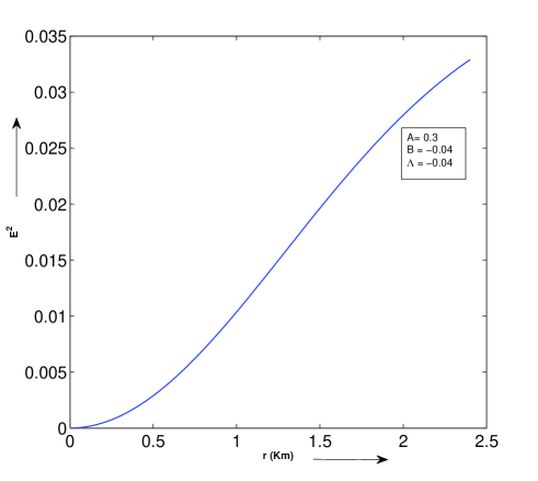
Figure 1: Variation of the energy-density ‘$\rho$’ (left) and the electric field intensity, ‘$E^{2}$’ (right) at the stellar interior.

II.1 Solutions admitting a linear EOS

Firstly we consider the linear EOS:

$$p_{r}=\alpha_{1}\rho+\alpha_{2},$$ (16)

where $\alpha_{1}$ and $\alpha_{2}$ are constant parameters. For the choice of (16), the system of Eqs. (2)-(5) can be solved analytically and we get

$$\nu(r) = C_{1}+\left[\alpha_{1}\left({A-B}\right)-B\right]r^{2}+\frac{8\pi\alpha_{2}}{A}e^{Ar^{2}},$$ (17)

$$p_{r}(r) = \frac{\alpha_{1}}{8\pi}\left({A-B}\right)e^{-Ar^{2}}+\alpha_{2},$$ (18)

$$p_{t}(r) = \frac{1}{8\pi}\left[\left(\alpha_{1}(A-B)-B\right)\left(\alpha_{1}(A-B)-(A+B)\right)r^{2}e^{-Ar^{2}}+\left(\alpha_{1}(A-B)-B\right)(e^{-Ar^{2}}+16\pi\alpha_{2}r^{2})\right.$$ (19)

$$\left.+64\pi^{2}\alpha_{2}^{2}r^{2}e^{Ar^{2}}+8\pi\alpha_{2}(1+Ar^{2})-Be^{-Ar^{2}}+2\Lambda\right].$$

where $C_{1}$ is integrating constant. The measure of anisotropy is given by

$$\Delta=p_{t}-p_{r} = \frac{1}{8\pi}\left[\left(\alpha_{1}(A-B)-B\right)\left(\alpha_{1}(A-B)-(A+B)\right)r^{2}e^{-Ar^{2}}+\left(A-B\right)\left(1+2\alpha_{1}\right)8\pi\alpha_{2}r^{2}\right.$$ (20)

$$\left.+64\pi^{2}\alpha_{2}^{2}r^{2}e^{Ar^{2}}-2Be^{-Ar^{2}}+2\Lambda\right].$$

It is a measure of the anisotropic pressure of the fluid comprising the charged star. This force due to the anisotropic nature is directed outward when $p_{t}>p_{r}$ $\Leftrightarrow$ $\Delta>0$ and inward if $p_{t}<p_{r}$ $\Leftrightarrow$ $\Delta<0$. $p_{t}=p_{r}$ i.e., $\Delta=0$ corresponds to the particular case of an isotropic pressure of the charged fluid star.

II.2 Solutions admitting a non-linear EOS

Secondly, we consider the non-linear EOS:

$$p_{r}=\beta_{1}\rho+\frac{\beta_{2}}{\rho},$$ (21)

where $\beta_{1}$ and $\beta_{2}$ are constant parameters and solving the system of equations (2)-(5) analytically we get

$$\nu(r) = C_{2}+\left[\beta_{1}\left({A-B}\right)-B\right]r^{2}+\frac{\beta_{2}}{A}\left(\frac{32\pi^{2}}{A-B}\right)e^{2Ar^{2}},$$ (22)

$$p_{r}(r) = \beta_{1}\left(\frac{A-B}{8\pi}\right)e^{-Ar^{2}}+\beta_{2}\left(\frac{8\pi}{A-B}\right)e^{Ar^{2}},$$ (23)

$$p_{t}(r) = \frac{1}{8\pi}\left[\left(\beta_{1}(A-B)-B\right)^{2}r^{2}e^{-Ar^{2}}+\left(\beta_{1}(A-B)-B\right)(1-Ar^{2})e^{-Ar^{2}}+\frac{\beta_{2}}{2}\left(\frac{128\pi^{2}}{A-B}\right)(1+3Ar^{2})e^{Ar^{2}}\right.$$ (24)

$$\left.+\frac{\beta_{2}}{4}\left(\frac{128\pi^{2}}{A-B}\right)r^{2}e^{Ar^{2}}\left(\beta_{2}\left(\frac{128\pi^{2}}{A-B}\right)e^{2Ar^{2}}+4\left(\beta_{1}(A-B)-B\right)\right)-Be^{-Ar^{2}}+2\Lambda\right].$$

where $C_{2}$ is also integrating constant and the measure of anisotropy is given by

$$\Delta=p_{t}-p_{r} = \frac{1}{8\pi}\left[\left(\beta_{1}(A-B)-B\right)^{2}r^{2}e^{-Ar^{2}}-\left(\beta_{1}(A-B)-B\right)Ar^{2}e^{-Ar^{2}}+3\beta_{2}A\left(\frac{64\pi^{2}}{A-B}\right)r^{2}e^{Ar^{2}}\right.$$ (25)

$$\left.+\frac{\beta_{2}}{4}\left(\frac{128\pi^{2}}{A-B}\right)r^{2}e^{Ar^{2}}\left(\beta_{2}\left(\frac{128\pi^{2}}{A-B}\right)e^{2Ar^{2}}+4\left(\beta_{1}(A-B)-B\right)\right)-2Be^{-Ar^{2}}+2\Lambda\right],$$

The measure of anisotropy vanishes i.e., $\Delta=0$ corresponds to the particular case which depend on the constant parameters.

III Junction conditions

The electrovaccum exterior space-time of the circularly symmetric static star is described by the charged BTZ black hole Ba$\tilde{n}$ados et al (1992); ccj can be written in the following form as

$$ds^{2}=-\left(-M_{0}-\Lambda{r^{2}}-Q^{2}\ln r\right)dt^{2}+\left(-M_{0}-\Lambda{r^{2}}-Q^{2}\ln r\right)^{-1}dr^{2}+r^{2}d\theta^{2},$$ (26)

where, the parameter $M_{0}$ is the conserved mass associated with asymptotic invariance under time displacements and the parameter Q is total charge of the black hole. At the boundary $r=R$, continuity of the metric potentials yield the following junction conditions:

$$e^{\nu(R)} = -M_{0}-\Lambda R^{2}-Q^{2}\ln R,$$ (27)

$$e^{-\mu(R)} = -M_{0}-\Lambda R^{2}-Q^{2}\ln R.$$ (28)

Across the boundary r = R of the star together with the condition that the radial pressure must vanish at the surface i.e., $p_{r}(r=R)=0$, help us to determine these constants. Now, using the metric function $\mu(r)=AR^{2}$, in Eq. (28), we obtain the following solutions

III.1 Solution for linear EOS

the constant $C_{1}$ and the radius of the star obtained from Eqs.(17)-(18)

$$A = -\frac{1}{R^{2}}\ln\left(-M_{0}-\Lambda R^{2}-Q^{2}\ln R\right),$$ (29)

$$C_{1} = \ln\left(-M_{0}-\Lambda r^{2}-Q^{2}\ln R\right)-(\alpha_{1}(A-B)-B)R^{2}-\frac{8\pi\alpha_{2}}{A\left(-M_{0}-\Lambda r^{2}-Q^{2}\ln R\right)},$$ (30)

$$R = \frac{1}{\sqrt{A}}\left[\ln\left(-\frac{\alpha_{1}}{\alpha_{2}}\left(\frac{A-B}{8\pi}\right)\right)\right]^{\frac{1}{2}}.$$ (31)

III.2 Solution for non-linear EOS

here also, the constant $C_{2}$ and the radius of the star obtained from Eqs.(22)-(23)

$$A = -\frac{1}{R^{2}}\ln\left(-M_{0}-\Lambda R^{2}-Q^{2}\ln R\right),$$ (32)

$$C_{2} = \ln\left(-M_{0}-\Lambda r^{2}-Q^{2}\ln R\right)-(\beta_{1}(A-B)-B)R^{2}-\frac{\beta_{2}}{A}\left(\frac{32\pi^{2}}{A-B}\right)e^{2AR^{2}},$$ (33)

$$R = \frac{1}{\sqrt{2A}}\left[\ln\left(-\frac{\beta_{1}}{\beta_{2}}\left(\frac{A-B}{8\pi}\right)^{2}\right)\right]^{\frac{1}{2}}.$$ (34)

IV Physical Analysis

Now, we are in a position to investigate the physically meaningful interior solution for static fluid spheres. In this case Einstein s gravitational field equations must satisfy certain physical requirements. Some of the physically acceptable conditions have been generally recognized to be crucial for anisotropic matter distribution Harrera et al (1997); M. K. Mak et al (2003) as:

$\bullet$ Inside the star $r<R$, the density $\rho$ and the pressure p are everywhere positive and finite.

$\bullet$ The space-time is assumed not to possess an event horizon i.e., $2m(r)<r$.

$\bullet$ The radial and tangential pressures should be decreasing functions of r.

$\bullet$ To keep the centre of the space-time regular, we enforce both $\rho^{\prime}_{r}(0)=p^{\prime}_{r}(0)=0$ and $p_{r}(0)=p_{t}(0)$.

$\bullet$ The gradients $\frac{d\rho}{dr}$ , $\frac{dp_{r}}{dr}$ and $\frac{dp_{t}}{dr}$ should be negative.

$\bullet$ The radial pressure $p_{r}$ must vanish but the tangential pressure $p_{t}$ may not vanish at the boundary r = R of the star.

$\bullet$ Radial and transverse sound velocity should be less than unity i.e. $0\leq v_{sr}^{2}(=\frac{dp_{r}}{d\rho})\leq 1$ and $0\leq v_{st}^{2}(=\frac{dp_{t}}{d\rho})\leq 1$.

The parameters can easily be adjusted to produce models where the speed of sound is much less than unity. The behavior of the model is illustrated best in terms of graphs of the matter variables and the gravitational potentials. Here, we are trying to discuss all the restriction for both cases step by step as given below:

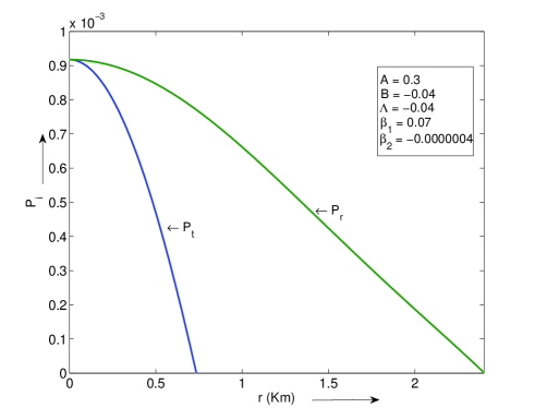
Figure 2: The radial and transverse pressure at the stellar interior for the linear (left) and non-linear (right) EOS.

IV.1 Stability for linear EOS

In linear case, we have

$$\frac{dp_{r}}{dr} = -\frac{\alpha_{1}}{4\pi}(A-B)Are^{-Ar^{2}}<~{}0,$$ (35)

$$v^{2}_{sr} = \frac{dp_{r}}{d\rho}=\alpha_{1},$$ (36)

$$v^{2}_{st} = \frac{dp_{t}}{d\rho}=\left[-\frac{\left(\alpha_{1}(A-B)-B\right)\left(\alpha_{1}(A-B)-(A+B)\right)(1-Ar^{2})}{A(A-B)}-\frac{64\pi^{2}\alpha_{2}^{2}}{A(A-B)}\left(1+Ar^{2}\right)e^{2Ar^{2}}\right.$$ (37)

$$\left.-\frac{8\pi\alpha_{2}}{(A-B)}e^{Ar^{2}}-\frac{\left(\alpha_{1}(A-B)-B\right)\left(16\pi\alpha_{2}e^{Ar^{2}}-A\right)}{A(A-B)}-\frac{B}{A-B}\right].$$

IV.2 Stability for non-linear EOS

In non-linear case, we have

$$\frac{dp_{r}}{dr} = -\beta_{1}\left(\frac{A-B}{4\pi}\right)Are^{-Ar^{2}}+\beta_{2}\left(\frac{16\pi}{A-B}\right)Are^{Ar^{2}}<~{}0,$$ (38)

$$v^{2}_{sr} = \frac{dp_{r}}{d\rho}=\beta_{1}-\beta_{2}\left(\frac{8\pi}{A-B}e^{Ar^{2}}\right)^{2},$$ (39)

$$v^{2}_{st} = \frac{dp_{t}}{d\rho}=\left[-\left(\beta_{1}(A-B)-B\right)^{2}\left(\frac{1-Ar^{2}}{A(A-B)}\right)+\left(\beta_{1}(A-B)-B\right)\left(\frac{2-Ar^{2}}{A-B}\right)-\frac{\beta_{2}}{2}\left(\frac{128\pi^{2}}{A-B}\right)\left(\frac{4+3Ar^{2}}{A-B}\right)e^{2Ar^{2}}\right.$$ (40)

$$\left.-\frac{B}{A-B}-\frac{\beta_{2}^{2}}{8}\left(\frac{128\pi^{2}}{A-B}\right)^{2}\left(\frac{2+3Ar^{2}}{A(A-B)}\right)e^{4Ar^{2}}-{\beta_{2}}\left(\beta_{1}(A-B)-B\right)\left(\frac{128\pi^{2}}{A-B}\right)\left(\frac{1+Ar^{2}}{A(A-B)}\right)e^{2Ar^{2}}\right].$$

Fig. (2), indicates that the pressure (radial and tangential) gradients are negative and monotonically decreasing functions of r. The necessary and sufficient criterion for the adiabatic speed of sound to be less than unity is satisfied by the suitable choice of the parameters shown in Fig. (3), however, Caporaso and Brecher G. Caporaso et al (2006) claimed that $\frac{dp}{d\rho}$ does not represent the signal speed. Therefore, if the speed of sound exceeds the speed of light, this does not necessary mean that the fluid is non-causal.

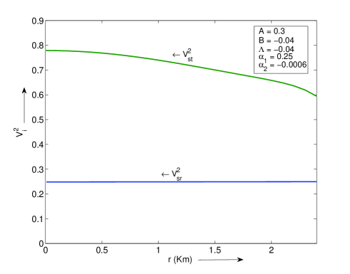
Figure 3: The variation of radial sound speed $v^{2}_{sr}$ and tangential sound speed $v^{2}_{st}$ sound speed at the stellar interior for the linear (left) and non-linear (right) EOS.

V Energy Conditions

The material composition of a physically reasonable charged fluid sphere has to obey the null energy condition (NEC), weak energy condition (WEC) and strong energy condition (SEC), at all points in the interior of a star if the following inequalities hold simultaneously :

$$\rho(r)+\frac{E^{2}}{8\pi}\geq 0,$$ (41)

$$\rho(r)+p_{r}(r)\geq 0,$$ (42)

$$\rho(r)+p_{t}(r)+\frac{E^{2}}{4\pi}\geq 0,$$ (43)

$$\rho(r)+p_{r}+p_{t}(r)+\frac{(E^{2}-\Lambda)}{8\pi}\geq 0.$$ (44)

It is to be noted in Table 1, that the set of constant parameters follow the restrictions and satisfy all the energy conditions shown in Fig. (4) for both linear and non-linear cases.

EOS	A(+ ve)	B (- ve)	$\Lambda$ (- ve)	$M_{0}$	Q	R(approx.)
linear	0.3	0.04	0.04	0.045	0.1	2.401
non-linear	0.3	0.04	0.04	0.045	0.1	2.404

Table 1: Values of the constant parameters.

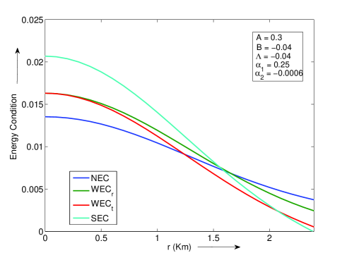
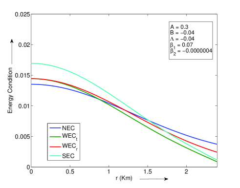
Figure 4: This figures shows that all energy conditions are satisfied at all points in the interior of the star solutions for both linear (left) and non-linear (right) EOS.

V.1 Gravitational effect on mass-radius relation and compactness

In this section, we study the maximum allowable mass-radius ratio for our model and the upper limit on the mass may be written as

$$8m(r)\equiv 1-e^{-Ar^{2}}-\Lambda r^{2}\leq 1-e^{-AR^{2}}-\Lambda R^{2}.$$ (45)

In Fig. (5), we have plotted $\frac{m(r)}{r}$ against $r$, which shows that the ratio $\frac{m(r)}{r}$ is an increasing function of the radial parameter. We observe that a constraint on the maximum allowed mass-radius ratio in our case falls within the limit of the (3+1)-dimensional isotropic fluid sphere i.e., $\left(\frac{m(r)}{r}\right)_{max}=0.0548$ $<\frac{4}{9}$, as obtained by Buchdahl H.A. Buchdahl et al (1959).

From Eq. (9), the compactness of the stellar configuration is given by

$$\mathcal{U}=\frac{m(r)}{r}\Bigl{\lvert}_{r=R}=\frac{1}{8r}\left(1-\Lambda r^{2}-e^{-Ar^{2}}\right),$$ (46)

and the surface redshift $\mathcal{Z}_{s}$ corresponding to the above compactness ($\mathcal{U}$) is obtain as

$$\mathcal{Z}_{s}=(1-8\mathcal{U})^{-\frac{1}{2}}-1,$$ (47)

where

$$\mathcal{Z}_{s}=\left[1-\frac{1}{r}\left(1-\Lambda r^{2}-e^{-Ar^{2}}\right)\right]^{-\frac{1}{2}}-1.$$ (48)

Thus, the maximum surface redshift $Z_{s}$ of our (2+1)-dimensional stellar configuration with radius R= 2.4 turns out to be $\mathcal{Z}_{s}=0.335$. For a static perfect fluid sphere in (3+1) dimensional gravity the surface redshift is less than Z = 2 H.A. Buchdahl et al (1959), however for anisotropic spheres this value may be larger B. V. Ivanov et al (2002).

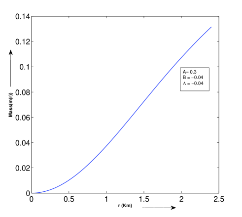
Figure 5: Variation of mass (left) and $\frac{m(r)}{r}$ (right) functions at stellar interior.

VI Equilibrium configuration

In Section III, we have matched the interior solution to the exterior charged BTZ metric with $p=\rho=0$, at a junction interface $\Sigma$, with junction radius r = R. In our case, the junction surface is an one dimensional ring of matter. One may also impose the boundary and regularity conditions, i.e., the metric coefficient are continuous across the surface, and their derivatives may not be continuous at the surface. In other words, the affine connections may be discontinuous at the boundary surface where the two boundary layers will both have a non-zero stress-energy. The magnitude of this stress-energy can be computed in terms of the second fundamental forms at the boundaries. So we adopt $\eta$, the Riemann normal coordinates at the junctions is positive in the manifold described by exterior Charged BTZ space-time and negative in the manifold described by the interior space-time with $x^{\mu}=(\tau,\phi,\eta)$, where $\tau$ represents the proper time on the shell. The second fundamental forms are given by:

$$K^{i\pm}_{j}=\frac{1}{2}g^{ik}\frac{\partial g_{kj}}{\partial\eta}\Bigl{\lvert}_{\eta=\pm 0}=\frac{1}{2}\frac{\partial r}{\partial\eta}\Bigl{\lvert}_{r=a}~{}g^{ik}\frac{\partial g_{kj}}{\partial r}\Bigl{\rvert}_{r=a}.$$ (49)

Since, $K_{ij}$ is not continuous at the junction, so the second fundamental forms with discontinuity are given by

$$\mathcal{K}_{ij}=K^{+}_{ij}-K^{-}_{ij}.$$ (50)

Now, from Lanczos equation in (2+1) dimensional space-time, the Einstein equations lead to

$$S^{i}_{j}=-\frac{1}{8\pi}\left(K^{i}_{j}-\delta^{i}_{j}K^{k}_{k}\right).$$ (51)

Considering circular symmetry, $K^{i}_{j}$ becomes

$$K^{i}_{j}=\left({\begin{array}[]{cc}K^{\tau}_{\tau}&0\\ 0&K^{\phi}_{\phi}\\ \end{array}}\right),$$ (52)

then one can obtain the surface stress energy tensor $S^{i}_{j}$ =diag$(-\sigma,-v)$ in terms of the energy density $\sigma$ and is surface pressure v, then Lanczos equation in (2+1)-dimensional space-time A. Banerjee et al (2013, 2013), becomes

$$\sigma = -\frac{1}{8\pi}\kappa_{\phi}^{\phi},$$ (53)

$$v = -\frac{1}{8\pi}\kappa_{\tau}^{\tau}.$$ (54)

Using the Eq. (52) in Eq. (51) we obtain

$$\sigma=-\frac{1}{8\pi R}\left[\sqrt{M_{0}-\Lambda R^{2}-Q^{2}\ln R}+e^{-\frac{AR^{2}}{2}}\right],$$ (55)

corresponding to the linear EOS

$$v=-\frac{1}{8\pi}\left[\frac{\Lambda R+\frac{Q^{2}}{2R}}{\sqrt{M_{0}-\Lambda R^{2}-Q^{2}\ln R}}+\{2\left(\alpha_{1}(A-B)-B\right)Re^{-\frac{AR^{2}}{2}}+16\pi\alpha_{2}Re^{\frac{AR^{2}}{2}}\}\right],$$ (56)

or, for non-linear EOS

$$v=-\frac{1}{8\pi}\left[\frac{\Lambda R+\frac{Q^{2}}{2R}}{\sqrt{M_{0}-\Lambda R^{2}-Q^{2}\ln R}}+\{2\left(\beta_{1}(A-B)-B\right)Re^{-\frac{AR^{2}}{2}}+4\beta_{2}\left(\frac{32\pi^{2}}{A-B}\right)Re^{\frac{3AR^{2}}{2}}\}\right],$$ (57)

where, we have set r = R. Lobo in his work F. Lobo et al (2006) shown that we can introduction of a thin shell on the junction hypersurface and it is possible to match the interior and exterior space-time without a thin shell. As we match second fundamental forms associated with the two sides of the shell, a crucial question arises in the form of the star s stability against collapse. Therefore, we must have a thin ring of matter component with above stresses so that the outer boundary exerts outward force to balance the inward pull of BTZ exterior. The energy density is negative in this junction ring which is similar to the (3 + 1) dimensional case M. Visser et al (1989).

VII Conclusion

In this work we have found a new type of charged star solution treating the matter distribution as anisotropic in nature admitting linear or nonlinear equation of state and for a specific field intensity. The starting point of this work is to assume a specific form of mass function m(r) and using this we found the energy density at the stellar interior. We match the star solution to the exterior charged BTZ solution and found the values of physically reasonable constant terms. All the solutions, which are obtained in both linear and nonlinear EOS are regular at the center and well behaved in the stellar interior except at the boundary where we propose a thin ring of matter content with negative energy density so as to prevent collapsing.

We observe that the energy density ($\rho$) and the pressures (radial and transverse) are positive and monotonically decreasing functions in the stellar interior, where the electric field intensity ($E^{2}$) and mass (m(r)) functions are positive and monotonically increasing within the radius of the star R=2.4 as shown in figures corresponding to the particular choices of the constant parameters given in Table 1. Consequently the solutions which we obtained in this paper has a simple analytical form which can be used to study a full collapsing model of a (2 + 1)-dimensional charged relativistic fluid sphere which is beyond the scope of this analysis.

References

- Bowers and Liang (1995) R. L. Bowers and E. P. T. Liang, Class. Astrophys. J. 188, 657 (1974).
- Ruderman (1995) R. Ruderman, Class. Ann. Rev. Astron. Astrophys 10, 427 (1972).
- Baados et al (1992) M. Baados, C. Teitelboim and J. Zanelli, Phys. Rev. Lett. 69, 1849 (1992).
- (4) C. Martinez, C. Teitelboim and J. Zanelli. Phys. Rev.D 61, 104013 (2000).
- Cruz and Zanelli (1995) N. Cruz and J. Zanelli, Class. Quantum Grav. 12, 975 (1995).
- Mann and Ross (1993) R.B. Mann and S.F. Ross, Phys. Rev. D 47, 3319 (1993).
- Garcí a and Campuzano (2003) A. A. Garcí a and C. Campuzano, Phys. Rev. D 67, 064014 (2003).
- D. Garfinkle (2003) D. Garfinkle, Phys.Rev. D 63, 044007 (2001).
- Paulo M. S (1999) Paulo M. S, Phys. Lett.B 467, 40 (1999).
- N. Ozdemiret al (2007) N. Ozdemir e-Print: arXiv: 0711.4732
- M. K. Maket al (1989) M. K. Mak and T. Harko, Int. J. Mod. Phys. D 13, 149 (2004).
- K. Komathirajet al (2007) K. Komathiraj and S.D. Maharaj, J. Math. Phys., 042501 (2007).
- R.Sharmaet al (2001) R.Sharma, S. Mukherjee and S.D.Maharaj, Gen. Relat. Gravit. 33, 999 (2001).
- L.K. Patelet al (1987) L.K. Patel, S.K. Koppar, Aust. J. Phys. 40, 441 (1987).
- L.K. Patelet al (1997) L.K. Patel, R.Tikekar and M.C.Sabu, Gen. Relat. Gravit. 29, 489 (1997).
- S.Thirukkaneshet al (1997) S.Thirukkanesh, and S.D. Maharaj Class. Quantum Grav. 23, 2697 (2006).
- V. Varelaet al (2010) V. Varela, F. Rahaman, S. Ray, K. Chakraborty and M. Kalam, Phys. Rev. D 82, 044052 (2010).
- Rahaman et al (2012) F. Rahaman, A.A. Usmain, S. Ray and S. Islam, Phys. Lett. B 717, 1 (2012).
- Sharma et al (2011) R. Sharma, F. Rahaman and I. Karar, Phys. Lett. B 704, 1 (2011).
- Banerjee et al (2013) A. Banerjee, F. Rahaman, K. Jotania, R. Sharma and Indrani Karar, Gen.Rel.Grav. 45, 717-726 (2013).
- Harrera et al (1997) L. Herrera, N. O. Santos, Phys. Reports 286 (1997) 53.
- M. K. Mak et al (2003) M. K. Mak and T. Harko, Proc. Roy. Soc. Lond., A 459: 393 408 (2003).
- G. Caporaso et al (2006) G. Caporaso and K. Brecher Phys. Rev. D 20, 1823-1831 (1979).
- H.A. Buchdahl et al (1959) H.A. Buchdahl, Phys. Rev. 116, 1027 (1959).
- B. V. Ivanov et al (2002) B. V. Ivanov, Phys. Rev. D 65, 104011 (2002).
- F. Lobo et al (2006) F. Lobo, Class. Quant. Grav. 23, 1525 (2006).
- M. Visser et al (1989) M. Visser, Nucl. Phys. B 328, 203 (1989).
- A. Banerjee et al (2013) F. Rahaman, A. Banerjee and I. Radinschi, Int. J. Theor. Phys. 51, 1680 (2011).
- A. Banerjee et al (2013) A. Banerjee, Int. J. Theor. Phys. 52, 2943 (2013).