Lyapunov Functions Family Approach to Transient Stability Assessment

Abstract

Analysis of transient stability of strongly nonlinear post-fault dynamics is one of the most computationally challenging parts of Dynamic Security Assessment. This paper proposes a novel approach for assessment of transient stability of the system. The approach generalizes the idea of energy methods, and extends the concept of energy function to a more general Lyapunov Functions Family (LFF) constructed via Semi-Definite-Programming techniques. Unlike the traditional energy function and its variations, the constructed Lyapunov functions are proven to be decreasing only in a finite neighborhood of the equilibrium point. However, we show that they can still certify stability of a broader set of initial conditions in comparison to the energy function in the closest-UEP method. Moreover, the certificates of stability can be constructed via a sequence of convex optimization problems that are tractable even for large scale systems. We also propose specific algorithms for adaptation of the Lyapunov functions to specific initial conditions and demonstrate the effectiveness of the approach on a number of IEEE test cases.

I Introduction

Ensuring secure and stable operation of large scale power systems exposed to a variety of uncertain stresses, and experiencing different contingencies are among the most formidable challenges that power engineers face today. Security and more specifically stability assessment is an essential element of the decision making processes that allow secure operation of power grids around the world. The most straightforward approach to the post-fault stability assessment problem is based on direct time-domain simulations of transient dynamics following the contingencies. Rapid advances in computational hardware made it possible to perform accurate simulations of large scale systems faster than real-time [1].

At the same time, the fundamental disadvantage of these approaches is their overall inefficiency. Reliable operation of the system implies that most of the contingencies are safe. And certification of their stability via direct simulations essentially wastes computational resources. Alternatively, the dynamics following non-critical scenarios could be proven stable with more advanced approaches exploiting the knowledge about the mathematical structure of the dynamic system. In the last decades numerous techniques for screening and filtering contingencies have been proposed and deployed in industrial setting. Some of the most common ideas explored in the field are based on the artificial intelligence and machine learning approaches [2, 3, 4, 5]. Most notable of them is the method of Ensemble Decision Tree Learning [6, 4] that is based on the construction of hierarchical characterization of the dangerous region in the space of possible contingencies and operating states.

An alternative set of approaches known under the name of direct energy methods were proposed in early 80s [7, 8, 9, 10] and developed to the level of industrial deployments over the last three decades [11, 12, 13, 14, 15, 16]. These approaches are based on rigorous analysis of the dynamical equations and mathematical certification of safety with the help of the so-called energy functions. Energy functions are a specific form of Lyapunov functions that guarantee the system convergence to stable equilibrium points. These methods allow fast screening of the contingencies while providing mathematically rigorous certificates of stability. At the same time, limited scalability and conservativeness of the classical energy methods limits their applicability and requires enhancement of the method with advanced algorithms for model reduction. Moreover, the algorithms rely on identification of unstable equilibrium point (UEP) of energy function which is known to be an NP-hard problem. In the recent decades a lot of research was focused on both extension of energy function to different system components [17, 13] and the improvement of algorithms that identify the UEPs [18, 19, 20]. Remarkably, the concept of controlling UEP [21] provides a practical and less conservative way to certify stability of the given fault-cleared state based on knowledge of the fault-on trajectory.

In this work we extend the ideas of classical energy method and propose its extension that alleviates some of the drawbacks discussed above. Basically, this paper makes two main contributions. First, we show that there exists a convex set of Lyapunov functions certifying the transient stability of a given power system, each corresponding to a different stability region estimate. Second, we introduce an adaptation algorithm to find the best suited Lyapunov function in the family to specific contingency situations. The proposed method can generally certify broader regions of stability compared to the closest-UEP method, and does not rely on knowledge of the fault-on trajectory as the controlling-UEP method. Also, the Lyapunov functions family is constructed via a sequence of Semi Definite Programming (SDP) problems that are known to be convex. Computational approaches for solving SDP problems have been in active development in the mathematical community over the last two decades and were recently successfully applied to a number of power systems, most importantly to optimal power flow [22, 23] and voltage security assessment [24] problems.

In addition to construction of Lyapunov functions family we propose several ways of their application to the problem of certification of power system stability. The first technique relies on minimization of possibly nonconvex Lyapunov functions over the flow-out boundary of a polytope in which the Lyapunov function is decaying. This technique certifies the largest regions of stability at the expense of reliance on non-convex optimization. Another alternative is to use only the convex region of the Lyapunov function, which allows more conservative but fast certification that can be done with polynomial convex optimization algorithm. The latter technique is similar to the recently proposed convex optimizations based on the classical direct energy method utilized to certify the security of the post-contingency dynamics [25]. Finally, as the last alternative we propose an analytical formulation that does not require any optimizations at all but also produces conservative stability certificates.

Applying these stability certificates, we discuss a direct method for contingency screening through evaluating the introduced Lyapunov functions at the post-fault state defining the contingency scenario. Unlike energy function approaches, the proposed approach provides us with a whole cone of Lyapunov functions to choose from. This freedom allows the adaptation of the Lyapunov functions to a specific initial condition or their family. We propose a simple iterative algorithm that possibly identifies the Lyapunov function certifying the stability of a given initial condition after a finite number of iterations.

Among other works that address similar questions we note recent studies of the synchronization of Kuramoto oscillators that are applicable to stability analysis of power grids with strongly overdamped generators [26, 27]. Also, conceptually related to our work are recent studies on transient stability [28] and [29] that propose to utilize network decomposition of power grids based on Sum of Square programming and port-Hamiltonian approach, respectively.

The structure of this paper is as follows. In Section II we introduce the transient stability problem addressed in this paper, and reformulate the problem in a state-space representation that naturally admits construction of Lyapunov functions. In Section III we explicitly construct the Lyapunov functions and corresponding transient stability certificates. Section IV explains how these certificates can be used in practice. Finally, in Section V we present the results of simulations for several IEEE example systems. We conclude in Section VI by discussing the advantages of different approaches and possible ways in improving the algorithms.

II Transient Stability of Power Systems

Faults on power lines and other components of power system are the most common cause for the loss of stability of power system. In a typical scenario disconnection of a component is followed by the action of the reclosing system which restores the topology of the system after a fraction of a second. During this time, however the system moves away from the pre-fault equilibrium point and experiences a transient post-fault dynamics after the action of the recloser. Similar to other direct method techniques, this work focuses on the transient post-fault dynamics of the system. More specifically, the goal of the study is to develop computationally tractable certificates of transient stability of the system, i.e. guaranteeing that the system will converge to the post-fault equilibrium.

In order to address these questions we use a traditional swing equation dynamic model of a power system, where the loads are represented by the static impedances and the $n$ generators have perfect voltage control and are characterized each by the rotor angle $\delta_{k}$ and its angular velocity $\dot{\delta}_{k}$. When the losses in the high voltage power grid are ignored the resulting system of equations can be represented as [30]

$$m_{k}\ddot{\delta}_{k}+d_{k}\dot{\delta}_{k}+\sum_{j}B_{kj}V_{k}V_{j}\sin(\delta_{k}-\delta_{j})-P_{k}=0$$ (1)

Here, $m_{k}$ is the dimensionless moment of inertia of the generator, $d_{k}$ is the term representing primary frequency controller action on the governor. $B_{kj}$ is the $n\times n$ Kron-reduced susceptance matrix with the loads removed from consideration. $P_{k}$ is the effective dimensionless mechanical torque acting on the rotor. The value $V_{k}$ represents the voltage magnitude at the terminal of the $k^{th}$ generator which is assumed to be constant.

Note, that more realistic models of power system should include dynamics of excitation system, losses in the network and dynamic response of the load. Although we don’t consider these effects in the current work, most of the mathematical techniques exploited in our work can be naturally extended to more sophisticated models of power systems. We discuss possible approaches in the end of the paper.

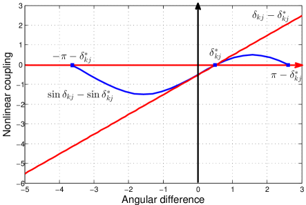
Figure 1: Bounding of nonlinear sinusoidal interaction by two linear functions as described in (10)

In normal operating conditions the system (1) has many stationary points with at least one stable corresponding to normal operating point. Mathematically, this point, characterized by the rotor angles $\delta_{k}^{*}$ is not unique, as any uniform shift of the rotor angles $\delta_{k}^{*}\to\delta_{k}^{*}+c$ is also an equilibrium. However, it is unambiguously characterized by the angle differences $\delta_{kj}^{*}=\delta_{k}^{*}-\delta_{j}^{*}$ that solve the following system of power-flow like equations:

$$\sum_{j}B_{kj}V_{k}V_{j}\sin(\delta_{kj}^{*})=P_{k}$$ (2)

Formally, the goal of our study is to characterize the so called region of attraction of the equilibrium point $\delta_{k}^{*}$, i.e. the set of initial conditions $\{\delta_{k}(0),\dot{\delta}_{k}(0)\}$ starting from which the system converges to the stable equilibrium $\delta_{k}^{*}$. To accomplish this task we use a sequence of techniques originating from nonlinear control theory that are most naturally applied in the state space representation of the system. Hence, we introduce a state space vector $x=[x_{1},x_{2}]^{T}$ composed of the vector of angle deviations from equilibrium $x_{1}=[\delta_{1}-\delta_{1}^{*}\dots\delta_{n}-\delta_{n}^{*}]^{T}$ and their angular velocities $x_{2}=[\dot{\delta}_{1}\dots\dot{\delta}_{n}]^{T}$. In state space representation the system can be expressed in the following compact form:

$$\dot{x}=Ax-BF(Cx),$$ (3)

with the matrix $A$ given by the following expression:

$$A=\left[\begin{array}[]{ccccc}O_{n\times n}&I_{n\times n}\\ O_{n\times n}&-M^{-1}D\\ \end{array}\right],$$ (6)

where $M$ and $D$ are the diagonal matrices representing the inertia and droop control action of the generators, $O_{n\times n}$ represents the zero and $I_{n\times n}$ the identity matrix of size $n\times n$. The other matrices in (3) are given by

$$B=\left[\begin{array}[]{ccccc}O_{n\times|\mathcal{E}|}\\ M^{-1}E^{T}B\\ \end{array}\right],C=[E\;\;O_{|\mathcal{E}|\times n}].$$ (9)

Here, $|\mathcal{E}|$ is the number of edges in the graph defined by the reduced susceptance matrix $B_{kj}$, or equivalently the number of non-zero non-diagonal entries in $B_{kj}$. $E$ is the adjacency matrix of the corresponding graph, so that $E[\delta_{1}\dots\delta_{n}]^{T}=[(\delta_{k}-\delta_{j})_{\{k,j\}\in\mathcal{E}}]^{T}$. We assume the increasing order of $j$ and $k$ for convenience of future constructions. Finally, the nonlinear transformation $F$ in this representation is a simple trigonometric function $F(Cx)=[(\sin\delta_{kj}-\sin\delta^{*}_{kj})_{\{k,j\}\in\mathcal{E}}]^{T}.$ The key advantage of this state space representation of the system is the clear separation of nonlinear terms that are represented as a “diagonal” vector function composed of simple univariate functions applied to individual vector components. This simplified representation of nonlinear interactions allows us to naturally bound the nonlinearity of the system in the spirit of traditional approaches to nonlinear control [31, 32, 33]. Our Lyapunov function construction is based on two key observations about the nonlinear interaction.

First, we observe that for all values of $\delta_{kj}=\delta_{k}-\delta_{j}$ such that $|\delta_{kj}+\delta_{kj}^{*}|\leq\pi$ we have:

$$0\leq(\delta_{kj}-\delta_{kj}^{*})(\sin\delta_{kj}-\sin\delta_{kj}^{*})\leq(\delta_{kj}-\delta_{kj}^{*})^{2}$$ (10)

This obvious property also illustrated on Fig. 1 allows us to naturally bound the nonlinear interactions by linear ones. Second, we note that in a smaller region $|\delta_{kj}|<\pi/2$ the function $\sin\delta_{kj}-\sin\delta_{kj}^{*}$ is monotonically increasing, a property that will play an essential role in proving the convexity of the level sets of Lyapunov functions in certain regions of the state space. In the following section we show how these properties of the system nonlinearity can be used to construct the Lyapunov functions certifying the transient stability of the system.

III Family of Lyapunov functions for stability assessment

The traditional direct method approaches are based on the concept of the so-called Energy function. The Energy function in its simplest version is inspired by the mechanical interpretation of the main equations (1):

$$E=\sum_{k}\frac{m_{k}\dot{\delta}_{k}^{2}}{2}-\sum_{\{k,j\}\in\mathcal{E}}B_{kj}V_{k}V_{j}\cos\delta_{kj}-\sum_{k}P_{k}\delta_{k}.$$ (11)

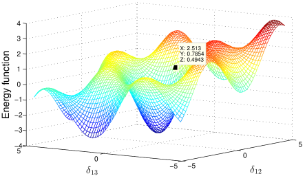
Figure 2: Energy function landscape depicted as a projection of the energy function into the surface defined by the angle differences $\{\delta_{12},\delta_{13}\}$

In this expression the first term in the right hand side represents the kinetic energy of the turbines and the second is the potential energy of the system stored in the inductive lines in the power grid network. The dissipative nature of the damping term in (1) ensures that the energy constructed in this way is always decreasing in time. Moreover, the energy plays a role of a Hamiltonian of the system defined for the natural momentum variables $p_{k}=m_{k}\dot{\delta}_{k}$, so the conservative part of the equations of motion (1) can be recovered via traditional Hamiltonian mechanics approach. This observation implies, that extrema of the potential energy in (11) are also the equilibrium points of the equations of motion (1). An example of Energy function for a simple $9$-bus system considered in section V is shown on Fig. 2. As one can see, the energy function possesses multiple extrema with only one of them corresponding to the actual equilibrium point.

Although, the decreasing nature of the energy function provides the most natural certificate of local stability, it is not the only function that can be shown to decrease in the vicinity of the equilibrium point. To illustrate this point qualitatively we first consider a trivial example of linear dynamics described by the equation $\dot{x}=Ax$. Whenever matrix $A$ is Hurwitz, the system has a trivial stable equilibrium $x=0$. Suppose now, that the left eigenvectors of $A$ are given by $u_{k}$ respectively, so that $u_{k}^{T}A=\lambda_{k}u_{k}^{T}$, where $\lambda_{k}$ is the corresponding eigenvalue. In this case, for every eigenpair there exists a Lyapunov function defined by $L_{k}(x)=x^{T}(u_{k}\bar{u_{k}^{T}}+\bar{u_{k}}u_{k}^{T})x\geq 0$, where $\bar{u_{k}}$ represents the complex conjugate of the vector. This Lyapunov function is simply the square amplitude of the state projection on the pair of eigenvectors corresponding to conjugate pair of eigenvalues. Obviously, as long as the system is stable this square amplitude is a strictly decaying function. Indeed, one can check that $dL_{k}/dt=2\operatorname{Re}(\lambda_{k})L_{k}\leq 0$. This construction suggests that any function of type $L(x)=\sum_{k}c_{k}L_{k}(x)$ with $c_{k}\geq 0$ is a Lyapunov function certifying the linear stability of $x^{*}=0$. In other words, the Lyapunov functions of stable linear systems form a simple orthant-type convex cone defined by inequalities $c_{k}\geq 0$.

In the context of energy functions, one can interpret the Lyapunov function $L_{k}$ as the energy stored in the mode $k$. Obviously for linear systems, the superposition principle implies that all these energies are strictly decaying functions. However, in the presence of nonlinearity, the energy of an individual mode is no longer strictly decaying, since the nonlinear interactions can transfer the energy from one mode to another. However, as long as the effect nonlienarity is relatively small it is possible to bound the rates of energy transfer and define smaller cone of Lyapunov functions that certify the stability of an equilibrium point.

For the system defined by (3) we propose to use the convex cone of Lyapunov functions defined by the following system of Linear Matrix Inequalities for positive, diagonal matrices $K,H$ of size $\mathcal{E}\times\mathcal{E}$ and symmetric, positive matrix $Q$ of size $2n\times 2n$:

$$\left[\begin{array}[]{ccccc}A^{T}Q+QA&R\\ R^{T}&-2H\\ \end{array}\right] \leq 0,$$ (14)

with $R=QB-C^{T}H-(KCA)^{T}$. For every pair $Q,K$ satisfying these inequalities the corresponding Lyapunov function is given by:

$$V(x)=\frac{1}{2}x^{T}Qx-\sum_{\{k,j\}\in\mathcal{E}}K_{\{k,j\}}\left(\cos\delta_{kj}+\delta_{kj}\sin\delta_{kj}^{*}\right)$$ (15)

Here, the summation goes over all elements of pair set $\mathcal{E}$, and $K_{\{k,j\}}$ denotes the diagonal element of matrix $K$ corresponding to the pair $\{k,j\}$. As one can see, the algebraic structure of every Lyapunov function is similar to the energy function (11). The two terms in the Lyapunov function (15) can be viewed as generalizations of kinetic and potential energy respectively. Moreover, the classical Energy function is just one element of the large cone of all possible Lyapunov functions corresponding to $K_{\{k,j\}}=B_{kj}V_{k}V_{j}$ and $Q$ given by the inertia matrix $M$.

In Appendix IX-A we provide the formal proof of the following central result of the paper. The Lyapunov function $V(x)$ defined by the equation (15) is strictly decaying inside the polytope $\mathcal{P}$ defined by the set of inequalities $|\delta_{kj}+\delta_{kj}^{*}|<\pi$. This polytope formally defines the region of the phase space where the nonlinearity can be bounded from above and below as shown in Eq. (10) and on Fig. 1. In other words, as long as the trajectory of the system in the state space stays within the polytope $\mathcal{P}$, the system is guaranteed to converge to the normal equilibrium point $\delta^{*}$ where the Lyapunov function acquires its locally minimum value. The convergence of Lyapunov function is proved in Appendix IX-B by using the LaSalle’s Invariance Principle. Here, the Lyapunov function $V(x)$ is possibly negative. However, if we add the constant $\sum_{\{k,j\}\in\mathcal{E}}K_{\{k,j\}}(\cos\delta_{kj}^{*}+\delta_{kj}^{*}\sin\delta_{kj}^{*})$ into the Lyapunov function $V(x),$ we will obtain a function which is positive definite in $\mathcal{P}$ and whose derivative is negative semidefinite in $\mathcal{P}.$ Hence, we can rigorously apply the LaSalle’s Invariance Principle.

We note that there may exists the case when the initial state lies inside $\mathcal{P}$, but after some time periods, the system trajectory escapes the polytope $\mathcal{P}$, and then the Lyapunov function is no longer decreasing. In order to ensure that the system will not escape the polytope $\mathcal{P}$ during transient dynamics we will add one condition to restrict the set of initial states inside $\mathcal{P}.$ Formally, we define the minimization of the function $V(x)$ over the union $\partial\mathcal{P}^{out}$ of the flow-out boundary segments $\partial\mathcal{P}_{kj}^{out}$:

$$V_{\min}=\mathop{\min}\limits_{x\in\partial\mathcal{P}^{out}}V(x),$$ (16)

where $\partial\mathcal{P}_{kj}^{out}$ is the flow-out boundary segment of polytope $\mathcal{P}$ that is defined by $|\delta_{kj}+\delta_{kj}^{*}|=\pi$ and $\delta_{kj}\dot{\delta}_{kj}\geq 0$. Given the value of $V_{\min}$ the invariant set of the Lyapunov function $V(x)$ where the convergence to equilibrium is certified is given by

$$\mathcal{R}=\left\{x\in\mathcal{P}:V(x)<V_{\min}\right\}.$$ (17)

Indeed, the decay property of Lyapunov function in the polytope $\mathcal{P}$ ensures that the system trajectory cannot meet the boundary segments $\{x:V(x)=V_{\min}\}$ and $\partial\mathcal{P}_{kj}^{out}$ of the set $\mathcal{R}.$ Also, once the system trajectory meets the flow-in boundary segment $\partial\mathcal{P}_{kj}^{in}$ defined by $|\delta_{kj}+\delta_{kj}^{*}|=\pi$ and $\delta_{kj}\dot{\delta}_{kj}<0,$ it can only go in the polytope $\mathcal{P}.$ Hence, the set $\mathcal{R}$ is invariant, and thus, is an estimate of the stability region.

Note that the stability region estimate is different for different choice of Lyapunov function. This allows for adaptation of the certificate to given initial conditions as well as the extension of the certified set by taking the union of estimates from all the Lyapunov functions. In the next section we describe the possible applications of this adaptation technique to the security assessment problem, while in section V and on the Fig. 3 we show that the invariant sets defined by the Lyapunov functions are generally less conservative in comparison to the classical Energy method (closest UEP method).

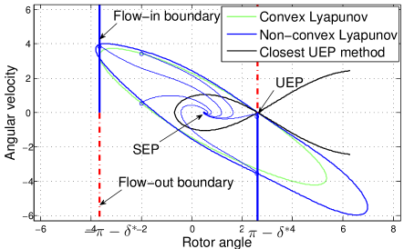
Figure 3: Comparison between invariant sets defined by convex and non-convex Lyapunov functions and the stability region obtained by the closest UEP energy method (black solid line). Invariant sets are intersection of the Lyapunov level sets (blue and green solid lines) and the polytope defined by $-\pi-\delta^{*}\leq\delta\leq\pi-\delta^{*}.$

We now discuss techniques to find the value of $V_{\min}$ for a given choice of Lyapunov function in the family. This task can be computationally difficult as both the function $V(x)$ and the boundary of the polytope $\partial\mathcal{P}$ are non-convex. In order to reduce the complexity of the stability certification we introduce three constructions of $V_{\min}$ that can be more computationally tractable, although resulting in more conservative stability region estimate at the same time. While the first construction relies on non-convex optimization and results in the largest estimate of stability region, the second one only uses convex region of the Lyapunov function and allows fast but more conservative certification. Finally, the third construction proposes an analytical approximation of $V_{\min}$ that does not require any optimizations but produces conservative stability certificate.

In particular, the first construction is based on the observation that $V_{\min}$ can be equivalently defined as the maximum value at which the largest Lyapunov function’s sublevel set does not intersect the flow-out boundary $\partial\mathcal{P}^{out}$ of the polytope $\mathcal{P}.$ With each sublevel set $\mathcal{S}(v)=\{x:V(x)<v\},$ we can find the following maximum value:

$$g(v) =\max_{\{k,j\}\in\mathcal{E},x\in\mathcal{S}(v)\cap\partial\mathcal{P}}\delta_{kj}\dot{\delta}_{kj}$$ (18)

A sublevel set that does not intersect the flow-out boundary $\partial\mathcal{P}^{out}$ of the polytope $\mathcal{P}$ is thus characterized by the inequality $g(v)<0.$ So, we can formally define the minimum value $V_{\min}$ as:

$$V_{\min} =\max_{g(v)<0}v.$$ (19)

Although this formulation may be easier to use in practice in comparison to the original defined by (16), the nonlinear constraint makes this problem non-convex, and difficult to solve for relatively large systems.

The second construction of $V_{\min}$ is based on the observation that the function $V(x)$ is convex in the polytope $\mathcal{Q}$ defined by the set of inequalities $|\delta_{kj}|\leq\pi/2$, or equivalently $\|\delta_{kj}\|_{\infty}\leq\pi/2$. So, all the sublevel sets that do not intersect the flow-out boundary $\partial\mathcal{Q}^{out}$ of the polytope $\mathcal{Q}$ will result in an invariant set as long as $\mathcal{Q}\subset\mathcal{P}$, condition that holds for most of the practically interesting situations. The convexity of the Lyapunov function helps us easily compute the maximum value $g^{convex}(v)$ defined as in (18) with $\partial\mathcal{P}$ replaced by $\partial\mathcal{Q}$ (see also [25] for the discussion of similar approach applied to the energy function based methods). Formally, one can then define the corresponding value of $V_{\min}$ as

$$V_{\min}^{convex} =\max_{g^{convex}(v)<0}v$$ (20)

Therefore, this certificate unlike the formers can be constructed in polynomial time.

The third construction of $V_{\min}$ is based on a lower approximation of the minimization of $V(x)$ taken place over the flow-out boundary $\partial\mathcal{P}^{out}$ of polytope $\mathcal{P}.$ In Appendix IX-C, we prove that the minimum value $V^{\{k,j\}}_{\min}$ of $V(x)$ on the boundary segment $\partial\mathcal{P}_{kj}^{out}$ of the polytope $\mathcal{P}$ is larger than $v_{\{k,j\}}=\frac{(\pm\pi-\delta_{kj}^{*})^{2}}{2C_{\{k,j\}}Q^{-1}C^{T}_{\{k,j\}}}-K_{\{k,j\}}(\cos(\pm\pi-\delta_{kj}^{*})+(\pm\pi-\delta_{kj}^{*})\sin\delta_{kj}^{*})-\sum_{\{u,v\}\neq\{k,j\}}K_{\{u,v\}}(\cos\delta_{uv}^{*}+\delta_{uv}^{*}\sin\delta_{uv}^{*}).$ As such, the value of $V_{\min}$ can be approximated by

$$V_{\min}^{approx}=\min_{\{k,j\}\in\mathcal{E}}v_{\{k,j\}}$$ (21)

where the minimization takes places over all elements of pair set $\mathcal{E}.$ This formulation of $V_{\min},$ though conservative, provides us with a simple certificate to quickly assess the transient stability of many initial states $x_{0},$ especially those near the stable equilibrium point $\delta^{*}.$

IV Direct Method for contingency screening

The LFF approach can be applied to transient stability assessment problem in the same way as other approaches based on energy function do. For a given post-fault state determined by integration or other techniques the value of $V_{0}=V(x_{0})$ can be computed by direct application of (15). This value should be then compared to the value of $V_{\min}$ calculated with the help of one of the approaches outlined in the previous section. Whenever $V_{0}<V_{\min}$ the configuration $x_{0}$ is certified to converge to the equilibrium point. If, however $V_{0}\geq V_{\min}$, no guarantees of convergence can be provided but the loss of stability or convergence to another equilibrium cannot be concluded as well. These configurations cannot be screened by a given Lyapunov function and should be assessed with other Lyapunov functions or other techniques at all.

The optimal choice among three different approaches for calculation of $V_{\min}$ is largely determined by the available computational resources. Threshold defined by (16) corresponds to the least conservative invariant set. However, the main downside of using (16) is the lack of efficient computational techniques that would naturally allow to perform optimization over the non-convex boundary of the polytope $\partial\mathcal{P}^{out}$. The second formulation of $V_{\min}$ in (20) based on convex optimizations makes it easier to compute by conventional computation techniques, but results in a more conservative invariant set. Finally, the third approach defined by (21) can be evaluated without any optimizations at all, but also provides more conservative guarantees.

The main difference of the proposed method with the energy method based approaches lies in the choice of the Lyapunov function. Unlike energy based approaches the LFF method provides a whole cone of Lyapunov functions to choose from. This freedom can be exploited to choose the Lyapunov function that is best suited for a given initial condition or their family. In the following we propose a simple iterative algorithm that identifies the Lyapunov function that certifies the stability of a given initial condition $x_{0}$ whenever such a Lyapunov function exits. The algorithm is based on the repetition of a sequence of steps described below.

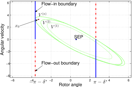
Figure 4: Adaptation of the Lyapunov functions to the contingency scenario over the iterations of the identifying algorithm in Section IV

First, we start the algorithm by identifying some Lyapunov function $V^{(1)}$ satisfying the LMIs (14), evaluate the function at the initial condition point $V^{(1)}(x_{0}),$ and find the value of $V_{\min}^{(1)}$. As long as the equilibrium point is stable such a function is probably guaranteed to exist, one possible choice would be the traditional energy function. Next, we solve again the problem (14) with an additional constraint $V^{(2)}(x_{0})<V_{\min}^{(1)}-\epsilon$, where $\epsilon$ is some step size. Note that the expression $V^{(2)}(x_{0})$ is a linear function of the matrices $Q,K,H$ to imposing this constraint preserves the linear matrix inequality structure of the problem. If a solution is found, two alternatives exit: either $V_{\min}^{(2)}>V^{(2)}(x_{0})$ in which case the certificate is found; or $V_{\min}^{(2)}\leq V^{(2)}(x_{0})$ in which case the iteration is repeated with $V^{(1)}$ replaced by $V^{(2)}$. In the latter, we have $V^{(2)}_{\min}\leq V^{(2)}(x_{0})<V_{\min}^{(1)}-\epsilon.$ Hence, the value of $V_{\min}$ is decreasing by at least $\epsilon$ in each of the iteration step, and thus, the technique is guaranteed to terminate in a finite number of steps. Once the problem is infeasible, the value of $\epsilon$ is reduced by a factor of $2$ until the solution is found. Therefore, whenever the stability certificate of the given initial condition exists it is possibly found in a finite number of iterations. Figure 4 illustrates the adaptation of Lyapunov functions over iterations to the initial states in a simple 2-bus system considered in Section V.

V Simulation results

V-A Classical 2 bus system

The effectiveness of the LFF approach can be most naturally illustrated on a classical $2$-bus with easily visualizable state-space regions. This system is described by a single 2-nd order differential equation

$$m\ddot{\delta}+d\dot{\delta}+a\sin\delta-P=0.$$ (22)

For this system $\delta^{*}=\arcsin(P/a)$ is the only stable equilibrium point (SEP). For numerical simulations, we choose $m=1$ p.u., $d=1$ p.u., $a=0.8$ p.u., $P=0.4$ p.u., and $\delta^{*}=\pi/6.$ Figure 3 shows the comparison between the invariant sets defined by convex and non-convex Lyapunov functions with the stability region obtained by the closest UEP energy method. It can be seen that there are many contingency scenarios defined by the configuration $x_{0}$ whose stability property cannot be certified by the closest UEP energy method, but can be guaranteed by the LFF method. Also, it can be observed that the non-convex Lyapunov function in (16) provides a less conservative certificate compared to the convex Lyapunov function, at the price of an additional computational overhead. For the obtained Lyapunov function, it can be computed that $V_{\min}=V_{\min}^{approx}=0.7748$ and $V_{\min}^{convex}=0.2073.$

Figure 4 shows the adaptation of the Lyapunov function identified by the algorithm in Section IV to the contingency scenario defined by the initial state $x_{0}.$ It can be seen that the algorithm results in Lyapunov functions providing increasingly large stability regions until we obtain one stability region containing the initial state $x_{0}$.

V-B Kundur 9 bus 3 generator system

Next, we consider the 9-bus 3-generator system with data as in [34]. When the fault is cleared, the post-fault dynamics of the system is characterized by the data presented in Tab. I.

Node	V (p.u.)	P (p.u.)
1	1.0566	-0.2464
2	1.0502	0.2086
3	1.0170	0.0378

TABLE I: Voltage and mechanical input

Node	1	2	3
1	1.181-j2.229	0.138+j0.726	0.191+j1.079
2	0.138+j0.726	0.389-j1.953	0.199+j1.229
3	0.191+j1.079	0.199+j1.229	0.273-j2.342

TABLE II: Reduced transmission admittance matrix

The reduced transmission admittance matrix is given in Tab. II, from which we have, $B_{12}\approx|Y_{12}|=0.739$ p.u., $B_{13}\approx|Y_{13}|=1.0958$ p.u., $B_{23}\approx|Y_{23}|=1.245$ p.u. By (2), we can calculate the stable equilibrium point: $\delta_{12}^{*}=-0.1588,\delta_{13}^{*}=-0.1005.$ For simplicity, we take $m_{k}=2$ p.u., $d_{k}=1$ p.u. Figure 2 shows the landscape of the energy function (11). From Fig. 2, it can be observed that the stability of the contingency defined by the initial state $\{\delta_{12}(0)=2.513,\delta_{13}(0)=0.7854\}$ cannot be guaranteed by the energy method since the initial energy, $E(0)=0.4943,$ is larger than the critical energy, which is about $0.196.$ Yet, we can find a Lyapunov function based on the proposed method that certifies the stability of contingency defined by the initial state $\{\delta_{12}(0)=2.513,\delta_{13}(0)=0.7854\},$ as can be interpreted from the strict decrease of Lyapunov function in Fig. 5(a). The convergence of the system from the initial state $\{\delta_{12}(0)=2.513,\delta_{13}(0)=0.7854\}$ to the equilibrium point is confirmed by simulation as in Fig. 5(b).

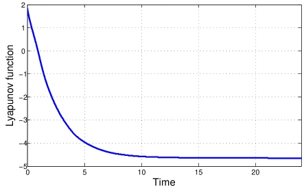
(a) Decrease of the Lyapunov function obtained by the identifying algorithm in Section IV

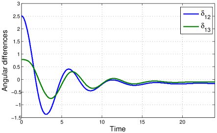
(b) Convergence of generators’ angles from the initial state $\{\delta_{12}(0)=2.513,\delta_{13}(0)=0.7854\}$ to the equilibrium $\{\delta_{12}^{*}=-0.1588,\delta_{13}^{*}=-0.1005\}$

Figure 5: Post-fault dynamics of a 9 bus 3 generator system

V-C New England 39 bus 10 generator system

To illustrate the scalability of the proposed approach, we consider the New England 39 bus 10 generator system, and evaluate the construction of Lyapunov function defined by (15). The equilibrium point is obtained by solving the power-flow like equations (2). The LMIs (14) are solved by the regular MATLAB sofware CVX to find the symmetric, positive matrix $Q$ of size $20\times 20$ and diagonal matrices $K,H$ of size $45\times 45.$ It takes about $2.5s$ for a normal laptop to solve these equations, by which the Lyapunov function $V(x)$ is achieved.

VI Discussion of the results

The Lyapunov Functions Family approach developed in this work is essentially a generalization of the classical energy method. It is based on the observation that there are many Lyapunov functions that can be proven to decay in the neighborhood of the equilibrium point. Unlike the classical energy function, the decay of these Lyapunov functions can be certified only in finite region of the phase space corresponding to bounded differences between the generator angles, more specifically for the polytope ${\cal P}$ defined by inequalities $|\delta_{ij}+\delta_{ij}^{*}|<\pi$. However, these conditions hold for practical purposes. Exceedingly large angle differences cause high currents on the lines and lead to activation of protective relays that are not incorporated in the swing equation model.

The limited region of state space where the Lyapunov function is guaranteed to decay leads to additional conditions incorporated in the stability certificates. In order to guarantee the stability one needs to ensure that the system always stays inside the polytope ${\cal P}$. We have proposed several approaches that ensure that this is indeed the case. The most straightforward approach is to inscribe the largest level set that does not intersect the flow-out boundary $\partial\mathcal{P}^{out}$ of the polytope ${\mathcal{P}}$. This approach provides the least conservative criterion, however the problem of inscription is generally NP-hard, similar to the problem of identification of closest unstable equilibria that needs to be solved in the traditional energy method. This approach is not expected to scale well for large scale systems. To address the problem of scalability we have proposed two alternative techniques, one based on convex optimization and another on purely algebraic expression that provide conservative but computationally efficient lower bounds on $V_{\min}$. Both of the techniques have polynomial complexity and should be therefore applicable even to large scale systems.

Our numerical experiments have shown that the LFF approach establishes certificates that are generally less conservative in comparison to the closest UEP energy approach and may be computationally tractable to large scale systems. Furthermore, the large family of possible Lyapunov functions allows efficient adaptation of the Lyapunov function to a given set of initial conditions. Moreover, the computational efficiency of the procedure allows its application to medium size system models even on regular laptop computers.

VII Path Forward

Although the techniques developed in this work address specific problem in transient stability assessment, the general strategy proposed in this work offers opportunities for development of computationally fast security assessment tools. We envision that security assessment where a database of stability and security of certificates is constructed offline using similar approaches that adopt the Lyapunov function for most common sets of contingencies. Although the construction of the certificate may take some significant time, its application to given system state can be done nearly instantaneously. So, a database of such certificates applicable to most common contingencies would allow the operator to certify security with respect to most common events, and focus the available computational resources on direct simulations of few contingencies that cannot be certified this way. At the same time, an extension of this approach similar to the one the authors have reported in [35] allows to certify that certain regions in operating conditions space are secure with respect to common contingencies. This approach offers a path for stability constrained optimization, as the operation in these safe regions may be enforced in optimization and planning tools.

There are several ways how the algorithm should be improved before it is ready for industrial deployment. First practical issue is the extension of the approach to more realistic models of generators, loads, and transmission network. Although this work demonstrated the approach on the simplest possible model of transient dynamics, there are no technical barriers that would prevent generalization of the approach. Unlike energy methods, our Lyapunov function construction does not require that the equations of motion are reproduced by variations of energy function. Instead, the algorithm exploits the structure of nonlienarity, which is confined to individual components interacting via a linear network. This property holds for all the more complicated models.

More specifically, incorporation of network losses can be easily accomplished by a simple shift of the polytope ${\mathcal{P}}$. Simple first order dynamic load models can be easily incorporated by extending the vector of nonlinear interaction function $F$. The most technically challenging task in extension of the algorithm is to establish an analogue of the bound (10) for higher-order models of generators and loads. This problem is closely related to the construction of the Lyapunov function that certifies the stability of individual generator models. The models of individual generators although being nonlinear have a relatively small order, that does not scale with the size of the system. Hence Sum-Of-Squares polynomial algebraic geometry approaches similar to ones exploited in [28] provide an efficient set of computational tools for bounding complicated but algebraic nonlinearity. We plan to explore this subject in the forthcoming works.

The next important question is the robustness of the algorithm to the uncertainty in system parameters, and initial state. As our algorithm is based on bound of the nonlinearity, it can naturally be extended to certify the stability of whole subsets of equilibrium points and initial post-fault states. Although these certificates will likely be more conservative, they could be precomputed offline and later applied to broader range of operating conditions and contingencies.

Finally, we note that the proposed algorithms in this paper are not applicable to give assessment for situations when the post-fault state is unstable. The extension of LFF method to certify the transient instability of power systems is a possible direction in our future research.

VIII Acknowledgements

This work was partially supported by NSF and MIT/Skoltech and Masdar initiatives. We thank Hung Nguyen for providing the data for our simulations and M. Chertkov for sharing the unpublished preprint [25]. We thank the anonymous reviewers for their careful reading of our manuscript and their many valuable comments and constructive suggestions.

IX Appendix

IX-A Proof of the Lyapunov function decay in the polytope $\mathcal{P}$

From (14), there exist matrices $X_{|\mathcal{E}|\times 2n},Y_{|\mathcal{E}|\times|\mathcal{E}|}$ such that $A^{T}Q+QA=-X^{T}X,QB-C^{T}H-(KCA)^{T}=-X^{T}Y,$ and $-2H=-Y^{T}Y.$ The derivative of $V(x)$ along (3) is:

$$\dot{V}(x)=\frac{1}{2}\dot{x}^{T}Qx+\frac{1}{2}x^{T}Q\dot{x}-\sum K_{\{k,j\}}(-\sin\delta_{kj}+\sin\delta_{kj}^{*})\dot{\delta}_{kj}$$

$$=0.5x^{T}(A^{T}Q+QA)x-x^{T}QBF+F^{T}KC\dot{x}$$

$$=-0.5x^{T}X^{T}Xx-x^{T}\big{(}C^{T}H+(KCA)^{T}-X^{T}Y\big{)}F$$

$$+F^{T}KC(Ax-BF)$$ (23)

Noting that $CB=0$ and $Y^{T}Y=2H$ yields

$$\dot{V}(x)=-0.5(Xx-YF)^{T}(Xx-YF)-(Cx-F)^{T}HF$$

$$=-0.5(Xx-YF)^{T}(Xx-YF)-\sum H_{\{k,j\}}g_{\{k,j\}},$$ (24)

where $g_{\{k,j\}}=\big{(}\delta_{kj}-\delta_{kj}^{*}-(\sin\delta_{kj}-\sin\delta_{kj}^{*})\big{)}(\sin\delta_{kj}-\sin\delta_{kj}^{*}).$ From Fig. 1, we have $g_{\{k,j\}}\geq 0$ for any $|\delta_{kj}+\delta_{kj}^{*}|\leq\pi.$ Hence, $\dot{V}(x)\leq 0,\forall x\in\mathcal{P},$ and thus the Lyapunov function $V(x)$ is decaying in $\mathcal{P}.$

IX-B Proof of the system convergence to the stable equilibrium

Consider an initial state $x_{0}$ in the invariant set $\mathcal{R}\subset\mathcal{P}.$ Then, $\dot{V}(x(t))\leq 0$ for all t. By LaSalle’s Invariance Principle, we conclude that $x(t)$ converges to the set $\{x:\dot{V}(x)=0\}.$ From (IX-A), if $\dot{V}(x)=0,$ then $\delta_{kj}=\delta_{kj}^{*}$ or $\delta_{kj}=\pm\pi-\delta_{kj}^{*}$ for all pairs $\{k,j\}.$ Hence, in the set $\{x:\dot{V}(x)=0\},$ the nonlinearity $F=0$ and the system (3) becomes $\dot{x}=Ax,$ from which it can be proved that $x(t)$ converges to some stationary points. Therefore, from $x_{0}$ the system converges to the stable equilibrium $\delta^{*}$ or to some stationary point $x^{*}$ lying on the boundary of $\mathcal{P}.$ Assume that $x(t)$ converges to some stationary point $x^{*}\in\partial\mathcal{P},$ then $x^{*}\in\partial\mathcal{P}^{out}$ ($\partial\mathcal{P}^{in}$ does not contain any stationary point since $\delta_{kj}\dot{\delta}_{kj}<0,\forall x\in\partial\mathcal{P}^{in}_{kj}$). By definition of $V_{\min}$ and $\mathcal{R}$, we have $V(x_{0})<V_{\min}\leq V(x^{*}),$ which is a contradiction with the fact that $V(x(t))$ is decaying in the invariant set $\mathcal{R}.$

IX-C Proof of the lower approximation of $V_{min}$

Let $I_{\{u,v\}}=\cos\delta_{uv}^{*}+\delta_{uv}^{*}\sin\delta_{uv}^{*}-\cos\delta_{uv}-\delta_{uv}\sin\delta_{uv}^{*},$ then

$$V^{\{k,j\}}_{\min}+\sum_{\{u,v\}\neq\{k,j\}}K_{\{u,v\}}(\cos\delta_{uv}^{*}+\delta_{uv}^{*}\sin\delta_{uv}^{*})$$

$$=\mathop{\min}\limits_{x\in\partial\mathcal{P}_{kj}^{out}}\Big{[}0.5x^{T}Qx-K_{\{k,j\}}\left(\cos\delta_{kj}+\delta_{kj}\sin\delta_{kj}^{*}\right)$$

$$\qquad\qquad\qquad+\sum_{\{u,v\}\neq\{k,j\}}K_{\{u,v\}}I_{\{u,v\}}\Big{]},$$ (25)

Note, that $I_{\{u,v\}}\geq 0,\forall x\in\mathcal{P},$ and the second term in the right hand side of (IX-C) is a constant on $\partial\mathcal{P}_{kj}^{out}.$ Hence,

$$V^{\{k,j\}}_{\min}+\sum_{\{u,v\}\neq\{k,j\}}K_{\{u,v\}}(\cos\delta_{uv}^{*}+\delta_{uv}^{*}\sin\delta_{uv}^{*})$$

$$\geq\mathop{\min}\limits_{x\in\partial\mathcal{P}_{kj}}(0.5x^{T}Qx)-K_{\{k,j\}}\left(\cos\theta_{kj}^{*}+\theta_{kj}^{*}\sin\delta_{kj}^{*}\right)$$

$$=\frac{(\theta_{kj}^{*})^{2}}{2C_{\{k,j\}}Q^{-1}C^{T}_{\{k,j\}}}-K_{\{k,j\}}\left(\cos\theta_{kj}^{*}+\theta_{kj}^{*}\sin\delta_{kj}^{*}\right),$$

with $\theta_{kj}^{*}=\pm\pi-\delta_{kj}^{*},$ and thus we obtain (21).

References

- [1] I. Nagel, L. Fabre, M. Pastre, F. Krummenacher, R. Cherkaoui, and M. Kayal, “High-Speed Power System Transient Stability Simulation Using Highly Dedicated Hardware,” Power Systems, IEEE Transactions on, vol. 28, no. 4, pp. 4218–4227, 2013.
- [2] L. Wehenkel, T. Van Cutsem, and M. Ribbens-Pavella, “An Artificial Intelligence Framework for On-Line Transient Stability Assessment of Power Systems,” Power Engineering Review, IEEE, vol. 9, no. 5, pp. 77–78, 1989.
- [3] A. A. Fouad, S. Vekataraman, and J. A. Davis, “An expert system for security trend analysis of a stability-limited power system,” Power Systems, IEEE Transactions on, vol. 6, no. 3, pp. 1077–1084, 1991.
- [4] M. He, J. Zhang, and V. Vittal, “Robust Online Dynamic Security Assessment Using Adaptive Ensemble Decision-Tree Learning,” Power Systems, IEEE Transactions on, vol. 28, no. 4, pp. 4089–4098, 2013.
- [5] Y. Xu, Z. Y. Dong, J. H. Zhao, P. Zhang, and K. P. Wong, “A Reliable Intelligent System for Real-Time Dynamic Security Assessment of Power Systems,” Power Systems, IEEE Transactions on, vol. 27, no. 3, pp. 1253–1263, 2012.
- [6] R. Diao, V. Vittal, and N. Logic, “Design of a Real-Time Security Assessment Tool for Situational Awareness Enhancement in Modern Power Systems,” Power Systems, IEEE Transactions on, vol. 25, no. 2, pp. 957–965, 2010.
- [7] M. A. Pai, K. R. Padiyar, and C. RadhaKrishna, “Transient Stability Analysis of Multi-Machine AC/DC Power Systems via Energy-Function Method,” Power Engineering Review, IEEE, no. 12, pp. 49–50, 1981.
- [8] A. N. Michel, A. Fouad, and V. Vittal, “Power system transient stability using individual machine energy functions,” Circuits and Systems, IEEE Transactions on, vol. 30, no. 5, pp. 266–276, 1983.
- [9] Varaiya, P. P and Wu, F. F. and Chen, R.-L., “Direct methods for transient stability analysis of power systems: Recent results,” Proc. IEEE, vol. 73, pp. 1703–1715, 1985.
- [10] N. A. Tsolas, A. Arapostathis and P. P. Varaiya, “A structure preserving energy function for power system transient stability analysis,” IEEE Trans. Circ. and Syst., vol. CAS-32, pp. 1041–1049, 1985.
- [11] I. A. Hiskens and D. J. Hill, “Energy functions, transient stability and voltage behavior in power systems with nonlinear loads,” IEEE Trans. Power Syst., vol. 4, pp. 1525–1533, 1989.
- [12] A. A. Fouad and V. Vittal, Power System Transient Stability Analysis: Using the Transient Energy Function Method. NJ: Prentice-Hall: JEnglewood Cliffs, 1991.
- [13] H.-D. Chang, C.-C. Chu, and G. Cauley, “Direct stability analysis of electric power systems using energy functions: theory, applications, and perspective,” Proceedings of the IEEE, vol. 83, no. 11, pp. 1497–1529, 1995.
- [14] A. R. Bergen and V. Vittal, Power System Analysis. New Jersey: Prentice Hall, 2000.
- [15] H.-D. Chiang, Direct Methods for Stability Analysis of Electric Power Systems, ser. Theoretical Foundation, BCU Methodologies, and Applications. Hoboken, NJ, USA: John Wiley & Sons, Mar. 2011.
- [16] R. Davy and I. A. Hiskens, “Lyapunov functions for multi-machine power systems with dynamic loads,” Circuits and Systems I: Fundamental Theory and Applications, IEEE Transactions on, vol. 44, 1997.
- [17] M. Ghandhari, G. Andersson, and I. A. Hiskens, “Control lyapunov functions for controllable series devices,” Power Systems, IEEE Transactions on, vol. 16, no. 4, pp. 689–694, 2001.
- [18] H.-D. Chiang and J. S. Thorp, “The closest unstable equilibrium point method for power system dynamic security assessment,” Circuits and Systems, IEEE Transactions on, vol. 36, no. 9, pp. 1187–1200, 1989.
- [19] C.-W. Liu and J. S. Thorp, “A novel method to compute the closest unstable equilibrium point for transient stability region estimate in power systems,” Circuits and Systems I: Fundamental Theory and Applications, IEEE Transactions on, vol. 44, no. 7, pp. 630–635, 1997.
- [20] L. Chen, Y. Min, F. Xu, and K.-P. Wang, “A Continuation-Based Method to Compute the Relevant Unstable Equilibrium Points for Power System Transient Stability Analysis,” Power Systems, IEEE Transactions on, vol. 24, no. 1, pp. 165–172, 2009.
- [21] H.-D. Chiang, F. F. Wu, and P. P. Varaiya, “A BCU method for direct analysis of power system transient stability,” Power Systems, IEEE Transactions on, vol. 9, no. 3, pp. 1194–1208, Aug. 1994.
- [22] J. Lavaei and S. H. Low, “Zero Duality Gap in Optimal Power Flow Problem,” Power Systems, IEEE Transactions on, vol. 27, no. 1, pp. 92–107, 2012.
- [23] R. Madani, S. Sojoudi, and J. Lavaei, “Convex Relaxation for Optimal Power Flow Problem: Mesh Networks,” Power Systems, IEEE Transactions on, no. 99, pp. 1–13, 2014.
- [24] D. K. Molzahn, V. Dawar, B. C. Lesieutre, and C. L. DeMarco, “Sufficient conditions for power flow insolvability considering reactive power limited generators with applications to voltage stability margins,” in Bulk Power System Dynamics and Control-IX Optimization, Security and Control of the Emerging Power Grid (IREP), 2013 IREP Symposium. IEEE, 2013, pp. 1–11.
- [25] S. Backhaus, R. Bent, D. Bienstock, M. Chertkov, and D. Krishnamurthy, “Efficient synchronization stability metrics for fault clearing,” to be submitted.
- [26] F. Dorfler and F. Bullo, “Synchronization and transient stability in power networks and nonuniform Kuramoto oscillators,” Control and Optimization, SIAM Journal on, vol. 50, no. 3, pp. 1116–1642, 2012.
- [27] F. Dorfler, M. Chertkov, and F. Bullo, “Synchronization in complex oscillator networks and smart grids,” Proceedings of the National Academy of Sciences, vol. 110, no. 6, pp. 2005–2010, 2013.
- [28] M. Anghel, J. Anderson, and A. Papachristodoulou, “Stability analysis of power systems using network decomposition and local gain analysis,” in 2013 IREP Symposium-Bulk Power System Dynamics and Control. IEEE, 2013, pp. 978–984.
- [29] S. Y. Caliskan and P. Tabuada, “Compositional Transient Stability Analysis of Multi-Machine Power Networks,” arXiv preprint arXiv:1309.5422, 2013.
- [30] J. Machowski, J. Bialek, and J. Bumby, Power system dynamics: stability and control. John Wiley & Sons, 2011.
- [31] V. M. Popov, “Absolute stability of nonlinear systems of automatic control,” Automation Remote Control, vol. 22, pp. 857–875, 1962, Russian original in Aug. 1961.
- [32] V. A. Yakubovich, “Frequency conditions for the absolute stability of control systems with several nonlinear or linear nonstationary units,” Avtomat. i Telemekhan., vol. 6, pp. 5–30, 1967.
- [33] A. Megretski and A. Rantzer, “System analysis via integral quadratic constraints,” Automatic Control, IEEE Transactions on, vol. 42, no. 6, pp. 819–830, 1997.
- [34] P. M. Anderson and A. A. Fouad, Power Systems Control and Stability (2nd ed.), ser. IEEE Press Power Engineering Series. Piscataway, NJ, USA: John Wiley & Sons, 2003.
- [35] T. L. Vu and K. Turitsyn, “Synchronization Stability of Lossy and Uncertain Power Grids,” in American Control Conference (ACC), 2015, accepted. IEEE, 2015.