Dynamical evolution of two associated galactic bars

Abstract

We study the dynamical interactions of mass systems in equilibrium under their own gravity that mutually exert and experience gravitational forces. The method we employ is to model the dynamical evolution of two isolated bars, hosted within the same galactic system, under their mutual gravitational interaction. In this study we present an analytical treatment of the secular evolution of two bars that oscillate with respect one another. Two cases of interaction, with and without geometrical deformation, are discussed. In the latter case, the bars are described as modified Jacobi ellipsoids. These triaxial systems are formed by a rotating fluid mass in gravitational equilibrium with its own rotational velocity and the gravitational field of the other bar. The governing equation for the variation of their relative angular separation is then numerically integrated, which also provides the time evolution of the geometrical parameters of the bodies. The case of rigid, non-deformable, bars produces in some cases an oscillatory motion in the bodies similar to that of a harmonic oscillator. For the other case, a deformable rotating body that can be represented by a modified Jacobi ellipsoid under the influence of an exterior massive body will change its rotational velocity to escape from the attracting body, just as if the gravitational torque exerted by the exterior body were of opposite sign. Instead, the exchange of angular momentum will cause the Jacobian body to modify its geometry by enlarging its long axis, located in the plane of rotation, thus decreasing its axial ratios.

1 Introduction

The dynamical interactions between different galactic components is of growing interest with regard to modelling the self-consistent evolution of a stellar system, since it may provide important clues on the formation and environmental conditions of such a system. Within this general subject, many attempts can be found in the literature to investigate the dynamics of a barred galactic system from several different standpoints. Abramyan et al. (1986) and Louis & Gerhard (1988) made the first trials to provide a theoretical framework within which the mutual evolution of two triaxial systems, namely the bar and bulge components of barred galaxies (Louis & Gerhard 1988) combined with other components (Abramyan et al. 1986), can be followed. The work by Louis & Gerhard (1988), based on Jeans’s theorem in extended phase space, provided some insights into oscillating systems governed by a periodically time-dependent gravitational potential, while the paper of Abramyan et al. (1986) considers the equilibrium conditions for both collisionless and fluid-dynamical models of a self-gravitating bulge within a complex system of bar, disc and halo. Martínez-Valpuesta et al. (2006) have analysed the evolution of a galactic bar, focusing on the vertical buckling instability that would lead to pronounced changes in the shape of the bulge, which would then appear as boxy/peanut-shaped giving rise to a pseudo double bar system; Weinberg & Katz (2007a, b) have investigated the dynamics of bar–halo interactions using perturbation theory and numerical experiments; Maciejewski & Athanassoula (2007, 2008) have analysed the orbits and trajectories of particles which form the backbone of nested bar systems; Debattista & Shen (2007) (hereafter DS07) and Shen & Debattista (2009) consider the case of a barred galaxy hosting a secondary bar. These authors, and others, have made substantial contributions to the setting of the problems, using N-body simulations in most cases, although the case of mutual interaction of two bars has not yet been a subject of study.

In this contribution we summarize the first results of an ongoing investigation into the matter with the aim at providing a new theoretical approach to the problem of dynamical interaction and evolution in stellar systems. We have purposely selected the case of double-bar systems given the increasing amount of observational evidence of their high relative frequency in the Universe (see Erwin 2008, and references therein, although this review focuses on galaxies where a smaller secondary bar is nested inside a larger primary bar), the different models available for their treatment and the evidence for a double-bar structure in the central region of the Milky Way. To this end, we have followed a purely analytical approach using the basic equations of classical mechanics and the treatment of ellipsoidal bodies in equilibrium with their own gravity (Lyttleton 1953; Chandrasekhar 1969).

It should be noted that our own galaxy, the Milky Way, most probably hosts a double-bar type structure at its centre—the long thin bar and the boxy bulge, whose detailed nature and very existence are the subject of some controversy. The rationale for the Milky Way being a barred galaxy has steadily gained acceptance following many discoveries concerning the morphology of the central regions of the Galaxy, mostly from detailed NIR star counts. The first evidence for a bar-like distribution of the stars was derived from the asymmetries in the infrared surface brightness maps (e.g. Matsumoto et al. 1982; Blitz & Spergel 1991; Dwek et al. 1995) and in source counts (Weinberg 1992; Hammersley et al. 1994; Stanek et al. 1994), which all show systematically more stars at positive galactic longitudes within $\displaystyle\ell<30^{\circ}$ and close to the Galactic plane compared to negative longitudes. The exact morphology of the inner Galaxy, however, is still controversial. While some authors refer to a fat structure, around 2.5 kpc in length with a position angle (PA) of 15– 30with respect to the Sun–Galactic Centre direction (Dwek et al. 1995; Nikolaev & Weinberg 1997; Stanek et al. 1997; Binney et al. 1997; Freudenreich 1998; Bissantz & Gerhard 2002; Babusiaux & Gilmore 2005), other researchers suggest that there is also a long thin bar, the in-plane bar, with a half-length of 4 kpc and a position angle of around $\displaystyle 45^{\circ}$ (Peters 1975; Weinberg 1992; Stanek et al. 1994; Benjamin et al. 2005). It is noteworthy that those authors supporting the $\displaystyle 23^{\circ}$ PA bar all examine the region at $\displaystyle|\ell|<12^{\circ}$, whereas those supporting the long bar with the larger PA are trying to explain counts for $\displaystyle 10^{\circ}<|\ell|<30^{\circ}$. It is also useful to mention that several authors in the first group assume that it is the boxy bulge of the central Galaxy which produces the bar-like structure seen in the observational data. This variety of standpoints is also present for the nature of the double bar structure in external galaxies possessing this feature. In Compere et al. (2014), we present some evidences for two different bar-like morphologies within the same galaxy.

The detailed geometrical morphology and luminosity function of this boxy bulge was delineated in López-Corredoira et al. (2005) by Bayesian inversion of the stellar statistics equation using 2MASS star counts. Analysing the TMGS $\displaystyle K$ -band star counts, Hammersley et al. (1994) and Calbet et al. (1995) initially posited the existence of a long bar of radius 4 kpc, with its closest tip at $\displaystyle\ell=27^{\circ}$ and the farthest at $\displaystyle\ell=-22^{\circ}$, thus indicating a PA of of $\displaystyle 75^{\circ}$. Calbet et al. (1996) claimed the existence of a dust lane preceding the bar at negative longitudes as expected for a rotating bar, which would explain the higher extinction observed in this region. The analysis of the TMGS database resulted in spectroscopic follow-up of selected samples. Thus Garzón et al. (1997) and López-Corredoira et al. (1999) reported a large excess of supergiants in the $\displaystyle\ell=27^{\circ}$ area, covered by the TMGS. Such regions form because of the concentrations of shocked gas where a galactic bar meets a spiral arm, as observed at the ends of the bars of face-on external galaxies. Thus, the presence of a massive star formation region is very strong supporting evidence for the presence of a bar in our Galaxy. Hammersley et al. (2000) made use of a preliminary data set of the TCS–CAIN survey in which the red-clump stellar population could be identified and then used as a standard candle for distance calculation. In so doing, it became clear to them that the geometry of the bar needed to be re-estimated to yield a revised PA of $\displaystyle 43^{\circ}$, after correcting the position of the farthest end of the bar, now at $\displaystyle\ell=-12^{\circ}$. New data analyses are also shown in López-Corredoira et al. (2007) and Cabrera-Lavers et al. (2007).

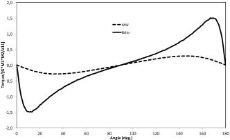
Figure 1: Variation of the torque with the angle between bars. Two cases are shown: solid line, labelled Bthin, is for two identical bars with $\displaystyle q_{2}=q_{3}=0.1$; and dashed line, labelled MW, represents a configuration similar to that of the Milky Way (see text), with $\displaystyle q_{2}=0.22$ and $\displaystyle q_{3}=0.04$, for the long bar, and $\displaystyle q_{2}=0.5$ and $\displaystyle q_{3}=0.4$, for the boxy bulge with its long axis half the length of that of the long bar. The torque is given in units of $\displaystyle G\times M_{1}\times M_{2}/a_{11}$, $\displaystyle a_{11}$ being the semi-axis of the first bar. The ripples in the graphs are due inaccuracies of the numerical integration method (see text).

It seems tf1.imely to investigate from a theoretical point of view the nature of the interactions between two bar-like bodies that coexist within the same area of a galaxy like ours, and this is the main objective of this paper. We start, as is customary, by analysing the problem focusing on the mutual interaction of the two bars isolated from the rest of the system. It is our purpose to extend the reach of this research by including additional material structures from the host galaxy (the stellar and interstellar disc, halo, etc.) in subsequent phases, which will be reported in due course.

2 The study case

The general gravitational interaction between two rotating bodies can be described via the interchange of angular momentum, governed by the run of the mechanical mutual torque exerted on both bodies. In this analysis, we follow the secular evolution of two isolated triaxial bars under their mutual influence. We assume, for the sake of simplicity, that both bars are of uniform density, not necessarily equal, rotate about the same single axis and through the same pivotal point and can be represented by triaxial ellipsoids, each with its own geometric parameters. Each bar can then be regarded as a solid body comprising a stellar population orbiting in trapped trajectories within each bar potential, which will be scaled to the geometry of the bar, always keeping the same figure. The only external interaction considered on each bar will be the gravitational torque created by the other bar.

In this way, we can write the equations for the run of both the torque, $\displaystyle\vec{\tau}$, and angular momentum, $\displaystyle\mathbf{L}$, as

$${\begin{array}[]{ccccccc}\vec{\tau}_{\mathrm{T}}=\vec{\tau}_{1}+\vec{\tau}_{2}=0&&\vec{\tau}_{\mathrm{T}}={d\mathbf{L}_{\mathrm{T}}}/{dt}\\ \vec{\tau}_{i}={d\mathbf{L}_{i}}/{dt}&&\mathbf{L}_{i}=\bar{\bar{I_{i}}}\mathbf{\Omega}_{i}\end{array}}$$ (1)

the magnitudes with the subscript ‘T’ pertaining to the system as a whole, and those with i to each of the bars. $\displaystyle\bar{\bar{I_{i}}}$ is the tensor of inertia of each bar and $\displaystyle\mathbf{\Omega_{i}}$, the angular velocity. Let us set the $\displaystyle Z$-axis as the axis of rotation so that the only component of interest for the intervening magnitudes is the third one, along the $\displaystyle Z$-axis, and the torque, angular momentum and angular velocities can be treated from now on as scalars, considering their components along the $\displaystyle Z$-axis only. The moment of inertia of interest is then the third component of the diagonal tensor of inertia written in the reference system of the ellipsoid principal axes.

$\displaystyle\begin{array}[]{lr}\includegraphics[angle={-90},width=212.47617pt]{dib2_nj_short_1.eps}&\includegraphics[angle={-90},width=212.47617pt]{dib2_nj_short_2.eps}\\ \includegraphics[angle={-90},width=212.47617pt]{dib2_nj_short_3.eps}&\includegraphics[angle={-90},width=212.47617pt]{dib2_nj_short_4.eps}\\ \includegraphics[angle={-90},width=212.47617pt]{dib2_nj_short_5.eps}&\includegraphics[angle={-90},width=212.47617pt]{dib2_nj_short_6.eps}\end{array}$

Figure 2: Evolution with time of several geometrical and dynamical parameters of two rigid bars for six different configurations. At the top of each panel the initial parameter set for each bar is given. $\displaystyle\Phi_{0}$ is the initial angle between bars, assuming always that bar 1 lies along the $\displaystyle X$-axis at the start. Units for the parameters are given in the text. Solid lines show the PAs, in red for bar 1 and in blue for bar 2; the green line is the relative angle between bars. Angles are plotted in the range [0,180] by replacing PA by 360-PA for PA $\displaystyle>$ 180. Dashed lines represent the angular velocities for each bar, with the same colour code, plotted against the secondary $\displaystyle Y$-axis.

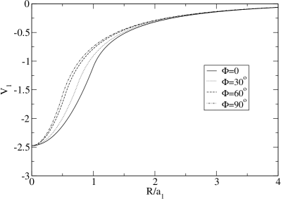
Figure 3: Potential created in the plane by a homogeneous ellipsoid with $\displaystyle q_{2}=0.5$, $\displaystyle q_{3}=0.25$ and semimajor axis $\displaystyle a_{1}$, following Eq. (10). Units are such that $\displaystyle GM/a_{1}=1$.

Hence, the governing equation for the evolution of the system is

$${\begin{array}[]{lll}\ddot{\Delta\Phi}&=&\left(\dot{\Omega}_{2}-\dot{\Omega}_{1}\right)\\ &=&\left({\frac{1}{{I_{2}}}+\frac{1}{{I_{1}}}}\right)\tau_{2}(\Delta\Phi)-\frac{{\mathrm{d}ln(I_{2})}}{{\mathrm{d}t}}\Omega_{2}+\\ &&+\frac{{\mathrm{d}ln(I_{1})}}{{\mathrm{d}t}}\Omega_{1}\end{array}}$$ (2)

which gives the variation of the relative position angle of the bars, $\displaystyle\Delta\Phi$ , in terms of the moment of inertia, $\displaystyle I_{i}$, angular velocities, $\displaystyle\Omega_{i}$, and gravitational torque, $\displaystyle\tau_{i}(=-\tau_{j\neq i})$. The two scalar moments of inertia, $\displaystyle I_{1}$ and $\displaystyle I_{2}$, are given by

$$I_{i}=\frac{1}{5}M_{i}(a_{1i}^{2}+a_{2i}^{2})=\frac{1}{5}M_{i}a_{1i}^{2}(1+q_{2i}^{2})$$ (3)

$\displaystyle a_{1i}$ and $\displaystyle a_{2i}$ being the semi-axes of the ellipses in the equatorial plane ($\displaystyle XY$) and the axial ratios with respect to $\displaystyle a_{1i},q_{2i}\equiv a_{2i}/a_{1i}$. The parameters $\displaystyle q_{3i}$, which will appear later, are also defined in this way, as the third axial ratios with respect to $\displaystyle a_{1i},a_{3i}/a_{1i}$.

The torque, its component along the $\displaystyle Z$-axis, can be expressed as a function of the azimuthal component of the force exerted by each elemental mass volume in bar $\displaystyle i$ to the bar $\displaystyle j$ at $\displaystyle\mathbf{r},F_{\Phi i}$, (see eq. (6) in López-Corredoira 2007) as:

$$\tau_{j}(\Delta\Phi)=\int_{V_{j}}{\mathrm{d}V\rho_{j}}F_{\Phi,i}(\mathbf{r})R$$ (4)

where $\displaystyle R$ is the radial component of the position vector $\displaystyle\mathbf{r}$ in the cylindrical coordinate system. Equation 4 is solved numerically for each of the study cases using a composite Simpson rule for multiple integrals. Details of the treatment of Eq. (4) are given in Appendix A. It needs to be stated, however, that the calculation of this multivariate integral using a rather simple quadrature produces small artificial fluctuations in the data of the type that can be seen in Figure 1 . This introduces small numerical errors at every integration step that can accumulate throughout the entire process. Thus, it is important to make the step length of the quadrature small enough to increase the accuracy of the result. This is even more crucial in ranges where the integrand experiences steeper variations. We have taken these actions into account in the integration.

In what follows we present some examples of the results obtained so far by integrating Eq. (2) in the two cases of rigid rotation (i.e. no variation in the moment of inertia with time is allowed) and deformable rotation, in which the moment of inertia varies with time. In both cases, the bars are assumed to be of uniform density. The case for heterogeneous bodies, under certain prescriptions, will be developed in a subsequent study.

2.1 The case for rigid rotation

This is the simplest case and can be studied quite easily with the help of Eq. (2), in which the last two terms have been dropped. A multistep method is then implemented by sequentially incrementing the time to follow the evolution of the double bar system. As initial parameters for the integration to proceed, we have selected the following:

• The masses, $\displaystyle M_{1}$ and $\displaystyle M_{2}$, of the bars, which remain unaltered in the integration.

• The lengths of the semi-axes, $\displaystyle(a_{1},a_{2},a_{3})$, of each bar, which are also unaltered during the evolution of the system.

• The initial angle, $\displaystyle\Delta\Phi$, between the major axis of bar 2 with respect to that of bar 1, and the initial rotational velocities of each bar.

The evolution of the system is controlled by Eq. (2), which can be rewritten in this case as

$$\ddot{\Delta\Phi}=\left(\dot{\Omega}_{2}-\dot{\Omega}_{1}\right)=\left({\frac{1}{{I_{2}}}+\frac{1}{{I_{1}}}}\right)\tau_{2}(\Delta\Phi)$$ (5)

and $\displaystyle\tau_{2}$ is computed for each relative angle following the prescriptions in Appendix A.

Given the initial parameters already detailed, the integration can now proceed. We show results for a parameter configuration representing the likely configuration of the central zone of the Milky Way, which comprises a long thin bar and a thick boxy bulge, whose geometries have been selected according to the structural parameters derived for the Galactic long bar and bulge (López-Corredoira et al. 2005, 2007; Sevenster et al. 1999): $\displaystyle M_{1}=6\times 10^{9},M_{2}=1.7\times 10^{10};a_{11}=4,q_{21}=0.22,q_{31}=0.04;a_{12}=2,q_{22}=0.5,q_{32}=0.4$; and with angular frequencies in the range $\displaystyle\Omega_{1},\Omega_{2}\in[0.03,1]$. Units are solar masses, kpc, rad Myr^-1, and sexagesimal degrees. We have also explored departures from this parameter space, part of which will be also shown here.

The evolution of the system is solely controlled by the variation of the torque with the angular separation of the bars. See Fig. 1 for the run of the torque for the case of two bars with a parameter set given in the caption. It has to be noted that the torque between the two bars is independent of these mass distributions being rigid or deformable and reflects only the action between the two distributions with a given configuration. The overall run of the torque is maintained in all the configurations, which does not depend on the angular speed of the bars. The angle at which the torque peaks is a function of the relative thickness of the two bars. It can be seen that the peak angle, with different sign at each side, roughly equals the angle at which the tip of the shortest bar, sketched for this purpose solely as a rectangle of half sides $\displaystyle a_{1i}$ and $\displaystyle q_{2i}\times a_{1i}$, abandons the location of the longest one, also represented in the same way for the calculation.

Results for this case of non-deformable bars are shown in Fig. 2 for six cases with mass ratios $\displaystyle M_{1}/M_{2}\approx[1/3,1/30]$, and $\displaystyle\Omega_{1},\Omega_{2}=[0.03,0.06,0.12,1.0]$. For the cases where the angular speed is similar, panels 1, 2 and 6 numbered from top to bottom and left to right, the lightest bar (bar 1 in the plots) remains trapped and oscillating around the more massive bar (bar 2), as also noted in Heller et al. (2001) but for the secondary nuclear gaseous bar. In these trapped cases the oscillation pattern remains the same. Bar 1 experiences the largest amplitude in variation of angular velocity, which increases with time. Bar 2 follows a similar pattern but at reduced amplitude. The amplitude in the oscillation of the relative angle also increases with time until the bars become coupled on the opposite side, when the overall motion pattern is repeated. Without these similar angular velocities, it is interesting to see how case 5 becomes a bounded system, in terms of developing oscillations, in contrast to case 3, sharing both the same frequencies of 0.03 and 0.12 rad Myr^-1 for bars 1 and 2. In the former, the mass of bar 2 is 10 times higher than in the latter case, which is sufficient to trap bar 1.

For the computation to produce trustworthy results, it is important to keep the time step within a tolerable range over which the intervening magnitudes in Eq. (5) can be considered as constant. This requires the number of integration steps to be very large to follow the evolution of the system over a sufficient number of oscillation periods. Since, as commented in Appendix A, we have selected a simplified method for solving the integral equation that gives the torque, we can decrease the size of the time step while keeping the computational time within reasonable limits. Throughout this paper, the time step has been selected in the range [0.1,0.5] Myr, which we have tested produces reliable results, without the need of implementing further corrective actions.

This rigid bar case hence produces a fixed oscillation pattern that lasts forever, as some sort of periodic oscillator, in the absence of external action on the system. This is a direct consequence of the conservation of both total angular momentum and energy that governs the evolution of the system as is developed in full in Appendix B.

The amplitude of the oscillations in angular velocity, and consequently in relative angle, depends on the mass ratios, being bigger for each bar the smaller this ratio is, and not on which bar rotates more rapidly, as can be seen by comparing the top right and bottom right panels: bar 1 is faster than bar 2, and the motion pattern is very much the same. The time period for cases 1, 2, 5 and 6 represented in Fig. 2 are 82.4, 91.1, 44.5 and 91.9 Myr, this period being the time length for the relative angle to perform a full oscillation. Examples 3 and 4 do not develop a periodic motion since the bars move at very different speeds and the mutual action does not significantly change the initial motion patterns.

2.2 The case for deformable rotation

To account for the variation of the moment of inertia, which follows the geometrical deformation of the bar with the interaction and time, the shape of the two bars has to be assigned to a given equilibrium figure. Triaxial ellipsoids seem to be the natural choice given the observed morphology of bars in external galaxies of a variety of orientations. Should the bars be isolated they would have been modelled as Jacobi ellipsoids, rotating fluid bodies in gravitational equilibrium with their own rotational velocity (Lyttleton 1953; Chandrasekhar 1969). Jacobi ellipsoids are homogeneous bodies and have a unique relation between the ratios of the axes, $\displaystyle q_{2}=a_{2}/a_{1}$ and $\displaystyle q_{3}=a_{3}/a_{1}$, being $\displaystyle(a_{1}\ a_{2}\ a_{3})$ the semi-axes of the bounding ellipsoids describing the bars, for the equilibrium to be at all possible, with which a unique angular velocity is associated for each figure. But in our case the bars form a coupled system in which each of the two must be in equilibrium not only with its own gravity but with the combined action of its own and the the other bar’s gravitational action. In this section we will develop an analytical approach, following closely that of the Jacobi ellipsoids, to derive the total gravitational potential acting on each bar and the resulting equations for the axes and rotational velocities of each bar. At this stage the bars will be considered as of homogeneous densities, but not as necessarily equal to each other.

$\displaystyle\begin{array}[]{c}\includegraphics[angle={0},width=203.80193pt]{jacmod_om_p1.eps}\\ \includegraphics[angle={0},width=203.80193pt]{jacmod_q2q3.eps}\\ \includegraphics[angle={0},width=203.80193pt]{jacmod_der.eps}\end{array}$

Figure 4: For several values of the density ratio $\displaystyle\rho_{2}/\rho_{1}$ and angular separation between the major axes of the two bars, $\displaystyle\Delta\Phi$, the variation of three representative parameters of bar 1 under the gravitational influence of bar 2 are plotted. The panels show: $\displaystyle\Omega_{1}/\sqrt{\pi G\rho_{1}}$ (top) ; $\displaystyle q_{21}$, $\displaystyle q_{31}$ (middle); $\displaystyle\delta_{1}$ (bottom) on top of the panel, and $\displaystyle\delta_{2}$ (see text for their definition). The two bars are set to be of equal axis lengths ($\displaystyle q_{2i}=0.520,q_{3i}=0.394$) and so would have the same rotational velocity ($\displaystyle\Omega_{i}^{2}/\pi G\rho_{i}=0.394$) in the Jacobian case.

This approach is somewhat simplistic but is sufficient for our purposes as we just try to discuss basic properties of the system of two bars. A global discussion of the interaction must also consider more realistic non-homogeneous cases and contain other elements, such as the interaction with other galactic components (disc, halo, etc.), and address the question of the deviations from equilibrium. The equilibrium and stability in self-gravitating systems such as bars in spiral galaxies (with violent relaxation, persistence of metaequilibrium states, slow collisional dynamics, phase transitions, etc.) has also been explored by other authors, getting in some cases only small departures of the system from equilibrium in an oscillation as a radial pulsation (Christodoulou et al. 1995; Chavanis et al. 2005). The relaxation time to reach the quasi-equilibrium states in the interaction of two bars is also interesting to explore, while the concept of relaxation is somewhat difficult to apply in our simple model, as we do not have orbital support in the bars, so that the internal kinematics of the system is simply not considered. In any case, double bar systems in galaxies are observed, and these may be regarded, at least to a first approximation, as ellipsoids in equilibrium.

When the bars are not rigid, the governing equation is Eq. (2), but in this case the moments of inertia of each bar, $\displaystyle I_{i}$, vary following Eq. (2) with the changes in the ellipsoid geometrical parameters, $\displaystyle(a_{1}\ a_{2}\ a_{3})$. That is to say, the interaction between the two systems implies the modification of the velocity patterns due to the interaction; also, both systems accommodate their own mass distribution to the new conditions to reach a new equilibrium state, which we have prescribed to be a triaxial ellipsoid. Taking this into account, each rotational velocity in Eq. (1) transforms into the following form:

$$\dot{\Omega}_{i}=\tau_{i}(\Delta\Phi)\left(I_{i}+\frac{\mathrm{d}I_{i}}{\mathrm{d}\Omega_{i}}\Omega_{i}\right)^{-1}$$ (6)

For ellipsoids, the moments of inertia are given by Eq. (3). Hence,

$$\dot{\Omega}_{i}=\frac{\tau_{i}(\Delta\Phi)}{I_{i}}\left(1+\frac{2\Omega_{i}}{a_{1i}}\frac{\partial a_{1i}}{\partial\Omega_{i}}+\frac{2q_{2i}\Omega_{i}}{1+q_{2i}^{2}}\frac{\partial{\kern 1.0pt}q_{2i}}{\partial{\kern 1.0pt}\Omega_{i}}\right)^{-1}$$ (7)

The gravitational potential for each of the bars can be obtained by adding the potential created by its own mass, $\displaystyle{\cal V}_{i}$, i.e. the potential of a homogeneous ellipsoid at points interior to itself, and the one due to the other bar, $\displaystyle{\cal V}_{j\neq i}$, i.e. the potential of an homogenous an ellipsoid at points interior or exterior to itself. Each of these follows the same equation, with different integration limits, which turn out to be:

$$\begin{array}[]{l}{\cal V}(\mathbf{x})=-\frac{3}{4}GM\int_{\nu(\mathbf{x})}^{\infty}\left[1-\sum_{j=1}^{3}\frac{x_{j}^{2}}{a_{j}^{2}+\lambda}\right]\frac{d\lambda}{\Delta(\lambda)},\\ \vspace*{-0.3cm}\\ \Delta^{2}(\lambda)=(a_{1}^{2}+\lambda)(a_{2}^{2}+\lambda)(a_{3}^{2}+\lambda)\\ \end{array}$$ (8)

$\displaystyle M$ and $\displaystyle a_{j}$ being the mass and semi-axes of the bar generating the potential, $\displaystyle x_{j}$ the $\displaystyle xyz$ coordinates of the position at which the potential is being evaluated ($\displaystyle\mathbf{x}$), and $\displaystyle\nu(\mathbf{x})$ is zero for points at the surface and interior to the bar and is the ellipsoidal coordinate of $\displaystyle\mathbf{x}$ for exterior points, i.e. the positive root of

$$\sum_{j=1}^{3}\frac{x_{j}^{2}}{a_{j}^{2}+\nu}=1$$ (9)

This potential can be expressed in a more convenient form, with the change $\displaystyle\lambda=a_{1i}^{2}\ \mu$, as

$$\begin{array}[]{l}{\cal V}_{i}(\mathbf{x})=\frac{3}{4}\frac{GM_{i}}{a_{1i}^{3}}\times\left[A_{i}[u_{i}(\mathbf{x})]x^{2}+B_{i}[u_{i}(\mathbf{x})]y^{2}+\right.\\ \vspace*{-0.3cm}\\ \left.\hskip 35.56593pt+C_{i}[u_{i}(\mathbf{x})]z^{2}-D_{i}[u_{i}(\mathbf{x})]a_{1i}^{2}\right]\\ \vspace*{-0.3cm}\\ A_{i}[u_{i}(\mathbf{x})]=\int_{u_{i}(\mathbf{x})}^{\infty}\frac{d\mu}{(1+\mu)\Delta^{\prime}_{i}(\mu)}\\ \vspace*{-0.3cm}\\ B_{i}[u_{i}(\mathbf{x})]=\int_{u_{i}(\mathbf{x})}^{\infty}\frac{d\mu}{(q_{2i}^{2}+\mu)\Delta^{\prime}_{i}(\mu)}\\ \vspace*{-0.3cm}\\ C_{i}[u_{i}(\mathbf{x})]=\int_{u_{i}(\mathbf{x})}^{\infty}\frac{d\mu}{(q_{3i}^{2}+\mu)\Delta^{\prime}_{i}(\mu)}\\ \vspace*{-0.3cm}\\ D_{i}[u_{i}(\mathbf{x})]=\int_{u_{i}(\mathbf{x})}^{\infty}\frac{d\mu}{\Delta^{\prime}_{i}(\mu)}\\ \vspace*{-0.3cm}\\ u_{i}(\mathbf{x})=\nu_{i}(\mathbf{x})/a_{1i}^{2}\ ;\ \Delta^{\prime}_{i}(\mu)^{2}\\ \hskip 25.6073pt=(1+\mu)(q_{2i}^{2}+\mu)(q_{3i}^{2}+\mu)\end{array}$$ (10)

where the subindex $\displaystyle i$ indicates that the magnitudes are evaluated using the parameters of bar $\displaystyle i$. Note that $\displaystyle A_{i}$, $\displaystyle B_{i}$, $\displaystyle C_{i}$ and $\displaystyle D_{i}$ are dimensionless, and that they do not depend on $\displaystyle a_{1i}$ for the points interior to the bar. $\displaystyle D_{i}$ cancels out in Eq. (12) as it does not depend on the spatial coordinates. In Fig. 3 there are examples of the shape of this potential evaluated in the XY plane of the bar and at several azimuths measured from the bar’s principal axis. It can be observed how this grows more or less linearly with radial distance from the centre of the ellipsoid until the surface of the body is reached ($\displaystyle R/a_{1}=1$), from which point it fades with distance, as expected.

Finally, we apply the condition for hydrostatic equilibrium of each of the rotating bar,

$${\cal V}_{i}(\mathbf{x_{i}})+{\cal V}_{j}(\mathbf{x_{i}})-\frac{1}{2}\Omega_{i}^{2}(x_{i}^{2}+y_{i}^{2})={\rm constant},$$ (11)

with $\displaystyle j\neq i$, which are combined with the requirement of the bars being triaxial ellipsoids to derive the governing equations of equilibrium of the rotating bar under the influence of its own gravity and that of the other bar. Hence Eq. (11) is developed for the points of the surface of each bar along the three axes, and with a second external bar separated by an angle $\displaystyle\Delta\Phi$, to get:

$$\begin{array}[]{l}A_{i}[0]+MR_{ji}\left[A_{j}[u_{ij1}]\cos^{2}(\Delta\Phi)+\right.\\ \left.+B_{j}[u_{ij1}]\sin^{2}(\Delta\Phi)\right]-E_{i}=\\ =q_{2i}^{2}\left\{B_{i}[0]+MR_{ji}\left[A_{j}[u_{ij2}]\sin^{2}(\Delta\Phi)\right.\right.\\ \left.+B_{j}[u_{ij2}]\cos^{2}(\Delta\Phi)\right]-E_{i}\big{\}}\\ =q_{3i}^{2}\left\{C_{i}[0]+MR_{ji}C_{j}[u_{ij3}]\right\}\\ MR_{ji}=\frac{M_{j}}{M_{i}}f_{ij}^{3},\ E_{i}=\frac{2\Omega_{i}^{2}a_{1i}^{3}}{3GM_{i}},\ f_{ij}=\frac{a_{1i}}{a_{1j}}\end{array}$$ (12)

where, again, $\displaystyle j\neq i$. The $\displaystyle u$ parameters in Eq. (12) are given by Eq. (9), followed by $\displaystyle u_{i}(\mathbf{x})=\nu_{i}(\mathbf{x})/a_{1i}^{2}$, applied in sequence to the three end points of the principal axes of bar $\displaystyle i$, using the parameters of bar $\displaystyle j$, to obtain:

$$\begin{array}[]{lll}u_{ij1}&=&\max\left\{0,\frac{1}{2}f_{ij}^{2}-\frac{1+q_{2j}^{2}}{2}+\sqrt{\Delta_{ij1}}\right\}\\ \Delta_{ij1}&=&\left[\frac{1+q_{2j}^{2}}{2}-\frac{1}{2}f_{ij}^{2}\right]^{2}-q_{2j}^{2}+f_{ij}^{2}\left[\sin^{2}(\Delta\Phi)+\right.\\ &&\left.+q_{2j}^{2}\cos^{2}(\Delta\Phi)\right]\\ u_{ij2}&=&\max\left\{0,\frac{1}{2}f_{ij}^{2}q_{2i}^{2}-\frac{1+q_{2j}^{2}}{2}+\sqrt{\Delta_{ij2}}\right\}\\ \Delta_{ij2}&=&\left[\frac{1+q_{2j}^{2}}{2}-\frac{1}{2}f_{ij}^{2}q_{2i}^{2}\right]^{2}-q_{2j}^{2}+f_{ij}^{2}q_{2i}^{2}\times\\ &&\times\left[\cos^{2}(\Delta\Phi)+q_{2j}^{2}\sin^{2}(\Delta\Phi)\right]\\ u_{ij3}&=&\max\left\{0,f_{ij}^{2}q_{3i}^{2}-q_{3j}^{2}\right\}\end{array}$$

In Eq. (12) it becomes clear that the influence of bar $\displaystyle j$ over bar $\displaystyle i$ is governed by the ratio of masses given by $\displaystyle MR_{ji}$. If set to 0, it is restricted to the case of Jacobi ellipsoids, and we get:

$$\Omega_{i}^{J}=\sqrt{\frac{3GM_{i}}{2a_{1i}^{3}}\frac{A_{i}[0]-q_{2i}^{2}B_{i}[0]}{1-q_{2i}^{2}}}$$ (13)

which corresponds to the rotational velocity of a Jacobi ellipsoid. By definition, $\displaystyle\partial A_{i}[0]/\partial a_{1i}=\partial B_{i}[0]/\partial a_{1i}=0$, and the quantity

$$\left[\frac{A_{i}[0]-q_{2i}^{2}B_{i}[0]}{1-q_{2i}^{2}}\right]=\int_{0}^{\infty}\frac{d\mu}{(1+\mu)(q_{2i}^{2}+\mu)\Delta_{i}(\mu)}$$

decreases when $\displaystyle q_{2i}$ increases. Hence, $\displaystyle\Omega_{i}^{J}\times\partial q_{2i}/\partial\Omega_{i}^{J}<0$, which means that the faster the rotation, the higher the length is and, in consequence, the eccentricity of the ellipsoids. Using Eq. (13), $\displaystyle(2\Omega_{i}^{J}/a_{1i})\times(\partial a_{1i}/\partial\Omega_{i}^{J})=-4/3$. Therefore, looking at Eq. (7), we see that $\displaystyle\dot{\Omega}_{i}^{J}/\tau_{i}<0$. The torque exerted by the bars on each other, in the case of pure Jacobi ellipsoids, produces a change in velocity of opposite direction to that of the torque. This means that the bars seem to repel each other, contrary to what happens in the rigid case, where the rotational velocity follows the course of the torque. Clearly, this is not an accurate model of the double bar configuration, as the potential of the other bar is not being considered in the equilibrium figure of the bar under study.

It is instructive to explore whether in the general case given by Eq. (12), which can be denoted as modified Jacobi ellipsoids following Miyamoto (1967), the same qualitative behaviour can be observed, as in the case of pure Jacobi ellipsoids. Figure 4 illustrates the scenario for a particular case with a given set of geometrical and kinematic parameters. It can be seen that $\displaystyle\delta_{1}\equiv(2\Omega_{i}/a_{1i})\times(\partial a_{1i}/\partial\Omega_{i})<-1$ and, as a matter of fact, very close to $\displaystyle-$4/3; and $\displaystyle\delta_{2}\equiv\Omega_{i}\times(\partial q_{2i}/\partial\Omega_{i})<0$ as well, which implies from Eq. (7) that $\displaystyle\dot{\Omega}_{i}/\tau_{i}<0$ as in the Jacobian case. In Fig. 4 the ratio of bar densities, which governs the influence of the external bar over the bar under study via the parameter $\displaystyle MR_{ji}$ in Eq. (12), runs up to 100. So even for a very strong influence of bar 2 on bar 1 this result is maintained, Which means that the same behaviour as seen in the Jacobian case is qualitatively followed here: the bars seem to repel each other, and this result is not dependent on the axial values $\displaystyle a_{ki}$.

We also see in the middle panel of Fig. 4 that $\displaystyle q_{21}$ is not very much affected with respect to the nominal value for the Jacobian case, the variation being roughly 10% at most, whereas the effect in $\displaystyle q_{31}$ is more conspicuous, reaching about 30%. But it is the rotation velocity, $\displaystyle\Omega_{1}$, which is affected the most, in terms of departure from the value at equilibrium of a Jacobi ellipsoid, which is located on the left of each of the three panels. This is particularly true for $\displaystyle\Delta\Phi\approx 0$ and large secondary bar masses, and reflects how that bar significantly increases the total gravitational attraction towards the centre of the galaxy, which must be compensated by a larger rotation velocity.

The evolution with time can be followed using Eqs (7) and (12), and the conservation of the total angular momentum. In this paper we have taken the approximation that bar 2 is much more massive than bar 1, so that their mutual influence is mostly reflected in bar 1. In this model, bar 2 can always be considered as a Jacobi ellipsoid with a well prescribed relationship between the geometry, i.e. the axes, and the rotational velocity, whereas bar 1 is a modified Jacobi ellipsoid described by Equation (12). We have also made the additional simplification of considering bar 2 as having fixed axes, which can be justified by the small impact of bar 1 on its geometry, as can be seen in Fig. 4/middle for small values of the density ratio. This small variation is even neglected for the ease of the calculationi. Finally, $\displaystyle\delta_{1}$ has been prescribed to take a fixed value of $\displaystyle-$4/3, which is roughly what we see in Fig. 4/bottom over an ample range of density ratios. Hence, for the sake of simplicity, bar 2 will be treated as a rigid bar described in section 2.1.

As initial parameters for the multistep integration method to proceed, we have selected the following:

• The masses, $\displaystyle M_{1}$ and $\displaystyle M_{2}$, of the intervening bars, which remain unaltered in the integration.

• The length of the axes, ($\displaystyle a_{1},a_{2},a_{3})$. Using Eqs 13, for bar 1, or 12, for bar 2, the initial rotational velocity can be determined.

• The initial angle, $\displaystyle\Delta\Phi$, between the major axes of the two bars.

Now the integration can proceed in steps of fixed amount of time, as mentioned before. The first task is to calculate the torque between the bars, as described in Appendix A. The torque between the two intervening bars is independent of the degree of deformability of the system, as it reflects the action between the two systems in a given structural configuration, since it is also independent of the relative speeds between bars. It is only dependent on the angle between bars and the given mass distribution. So the prescriptions in Appendix A provide the recipe for the torque, whose run will follow the pattern as in Figure 1. Next, Eq. (7), on which the derivatives are numerically calculated, provides the new value for the rotational velocity of bar 1, whereas the corresponding value for bar 2 comes directly from the torque (see Eq. (1). Finally, Eq. (12) gives the new axes for bar 1, while those of bar 2 are fixed. The whole process is repeated for a number of time steps to derive the evolution of the double bar system.

In Fig. 5, we see the evolution of bar 1 for a case with initial morphology $\displaystyle a_{11}=4,q_{21}=0.12,q_{31}=0.115$; and bar 2 with a fixed values of $\displaystyle a_{12}=3,q_{22}=0.520,q_{32}=0.394$ (lengths in kpc). The initial separation is $\displaystyle\Delta\Phi=30^{\circ}$, and masses $\displaystyle M_{1}$ and $\displaystyle M_{2}$ equal to $\displaystyle 3\times 10^{9}$ M_⊙ and $\displaystyle 2\times 10^{10}$ M_⊙ respectively. The time step for the integration has been set to 0.5 Myr. In this case the density ratio is initially 0.94, from which no conclusions can be derived by looking at Fig. 4, as the geometry of the bars are quite different. It is the mass ratio, which remains constant at 6.67 (the figure for $\displaystyle MR_{21}$ in Eq. (12)), which sets the validity of the simplifying assumptions explained before. In Fig. 5 it is seen how at first bar 1 decreases its size and increases its angular velocity as a result of the initial repulsive torque produced by bar 2, which quickly becomes $\displaystyle\Omega_{1}>\Omega_{2}$. This decrease in size of bar 1 is approximately constant in aspect ratio, as the major axis decreases by a factor greater than two while the $\displaystyle q$-axial ratios experienced minor changes. It can also be seen how the angular separation initially becomes smaller than the initial setting owing to $\displaystyle\Omega_{2}$ being larger than $\displaystyle\Omega_{1}$, a situation that is rapidly inverted by the action between the bars.

Soon after this episode of minimal size of bar 1, which corresponds to the maximum of rotational velocity, bar 1 quickly starts to approach the opposite end of bar 2, owing to its high relative velocity, and begins to experience a torque that tends to reverse the motion of bar 1 with respect to bar 2. $\displaystyle\Omega_{1}$ decreases rapidly until it becomes smaller than $\displaystyle\Omega_{2}$, when the bars start to invert their relative movement. This decrease in $\displaystyle\Omega_{1}$ is accompanied by an increase in $\displaystyle a_{11}$, which again happens with approximately constant aspect ratio. The result is a periodic oscillation between the states of minimum size–maximum angular velocity and maximum size–minimum angular velocity.

In Fig. 6 another configuration of a double bar system is explored, now with the two bars initially sharing the same geometry, which remains fixed for bar 2. At the beginning, the morphology of bar 1 is given by $\displaystyle a_{11}=3$ kpc, $\displaystyle q_{21}=0.12,q_{31}=0.115;a_{12}=3$. The initial separation is $\displaystyle\Delta\Phi=-30^{\circ}$, and masses $\displaystyle M_{1}=3\times 10^{9}$ M_⊙ and $\displaystyle M_{2}=2\times 10^{10}$ M_⊙, as in the previous case. The time step for the integration has been set to 0.1 Myr, as this configuration shows higher complexity. In this case of equal geometry the initial density ratio of 0.15 permits the use of Fig. 4 to ascertain the relative influence of each opposite bar.

At the beginning, the size of bar 1 grows and its aspect changes quite strongly: $\displaystyle q_{21}$ becomes smaller whereas $\displaystyle q_{31}$ increases, which makes the vertical axis larger than the second axis. The rotation during this episode slows down and comes close to stopping due to the positive torque. The angular separation of the two bars increases as the faster rotation of bar 2 tends to get bar 1 closer to the other end. As this is happening, the torque becomes smaller because of the larger separation and bar 1 becomes reduced in size, recovering angular velocity. As before, the change in size is accompanied by a substantial variation in aspect, as $\displaystyle q_{21}$ and $\displaystyle q_{31}$ vary in an opposite sense by a factor greater than two. As the bars continue approaching, the torque increases and the rotation of bar 1 also increases accordingly until the bars reach their minimum separation in which the larger torque pushes bar 1 to a much faster rotation, over that of bar 2, which recovers the original location of the bars. The system then develops in a periodic oscillation as in the case of Figure 5. The case appears more complex because of the variation of the axial ratios is here more important, taking a large factor of the angular momentum interchange. The shape of the global system is not exactly the same in each period of the oscillation in Fig. 6, but this is most probably due to inaccuracies in the numerical calculations, which we will improve in future papers. As far as we can see, extending the evolution of the system to a much larger time period than shown in Fig. 6, the system is bounded between the two status of maximum and minimum angular separation, while the exact details of the interaction would necessitate also accounting for the deformations of bar 2.

$\displaystyle\begin{array}[]{l}\includegraphics[angle={0},width=203.80193pt]{evol1a_n.eps}\\ \includegraphics[angle={0},width=203.80193pt]{evol1b_n.eps}\end{array}$

Figure 5: Evolution of two bars with $\displaystyle M_{1}=3\times 10^{9},M_{2}=2\times 10^{10}$ solar masses and initial parameters for bar 1: $\displaystyle a_{11}=4$ kpc, $\displaystyle q_{21}=0.120,q_{31}=0.115$; and a fixed geometry for bar 2 of $\displaystyle a_{12}=3$ kpc, $\displaystyle q_{22}=0.520,q_{32}=0.394$, with initial velocity of $\displaystyle\Omega_{2}^{2}/\pi G\rho_{2}=0.316$ (Jacobi ellipsoid); $\displaystyle\Delta\Phi=30^{\circ}$ as initial value. Top: evolution of the angular separation, in the range [0, $\displaystyle\pi$] and the angular velocities. Bottom: evolution of the axial ratios and semimajor axis of bar 1.

The two cases depicted in Figs 5 and 6 both share the same feature in the motion pattern of bar 1, the lightest of the two bars and the live one in the simulations. Since the two cases correspond to configurations in which bar 1 remains trapped with an oscillatory motion around bar 2 ($\displaystyle\Delta\Phi$ is confined in a given range) and always revolving in the same sense ($\displaystyle\Omega_{1}$ does not change its sign), two different events of alignment and perpendicularity can be distinguished. Initially, bar 2 gets an impulse with different sign with respect to its rotational velocity in the two examples. While for the case depicted in Fig. 5 the repulsion between the bars pushes to increase the frequency; in the case of Fig. 6 the torque slows down the motion of bar 2. This is due solely to the different initial location of the two bars in the examples. The change in angular velocity is accompanied by a change in opposite sense in bar size ($\displaystyle a_{11}$), as dictated by Equation (6). In the first example, bar 1 keeps increasing the speed and decreasing the size, moving until the closest approach on the other side and both bars become perpendicular to each other, when the mutual torque inverts its sign and bar 1 starts to brake its rotation and increases its size accordingly. Bar 1 becomes slower than bar 2 and the two bars tend towards separation. The perpendicular alignment in this motion marks the starts of the acceleration and size decrease of bar 1. The pattern is then repeated. So the status of the living bar in the positions close to being in alignment and orthogonal alternates during the motion pattern. Perpendicularity corresponds alternately to maximum (minimum) and minimum (maximum) rotation speed (size). In the second example, Fig. 6, the situation is similar but, owing to the different initial relative position, the evolution starts reaching first the status of minimum speed, and maximum size, of the living bar when the two bars are perpendicular to each other.

$\displaystyle\begin{array}[]{l}\includegraphics[angle={0},width=203.80193pt]{evol2a_n.eps}\\ \includegraphics[angle={0},width=203.80193pt]{evol2b_n.eps}\end{array}$

Figure 6: Evolution of two bars with $\displaystyle M_{1}=3\times 10^{9},M_{2}=2\times 10^{10}$ solar masses, and initial parameters: $\displaystyle a_{11}=3$ kpc, $\displaystyle q_{21}=0.120,q_{31}=0.115$; and a fixed geometry for bar 2 equals to that of the initial bar 1, which implies an initial velocity of $\displaystyle\Omega_{2}^{2}/\pi G\rho_{2}=0.0773$ (Jacobi ellipsoid); $\displaystyle\Delta\Phi=-30^{\circ}$ as initial value. Panels as in Figure 5.

To compare the predictions of the approach presented in this paper against $\displaystyle N$-body simulations, we have prepared a third configuration following the figures of DS07. This simulation, whose results are shown in Fig. 7, attempts to model a small secondary bar (bar 1) embedded within a larger and more massive primary bar (bar 2). In this case, bar 1 is always at the interior of bar 2, due to its small size, hence both potentials in Eq. (11) are calculated at interior points. As seen in Fig. 7, the result is that bar 1 develops an oscillatory motion pattern, with period of 20 Myr, much in the same way as fig. 2 of DS07, once B1 and B2 have been set. In this case, $\displaystyle\Omega_{1}$ is always faster than $\displaystyle\Omega_{2}$, as in DS07, so bar 1 is revolving around bar 2 and there is no alternating of maximum and minimum frequency between the positions of perpendicularity or alignment. The peak of rotation speeds of bar 1 always coincides with the bars being perpendicular and the minimum value, with the bars in alignment. This is contrary of what happens in the runs of DS07, where the small bar gets its maximum speed when the two bars align, which also coincides with the minima of the Fourier $\displaystyle m=2$ amplitude. This contradictory result can be attributed to the prescriptions of the modified Jacobi ellipsoid model, which acts as if the torque between the two bodies were of reversed sign. So the opposite results between DS07 and this paper in the locus of the maxima/minima of the rotation speeds was in a way expected. Except for this, the trend of the motion of the smaller bar is quite similar in both models, considering the rotation period and the amplitude of the oscillations. Further commonalities cannot be expected in view of the large difference in the conditions of the two scenarios.

$\displaystyle\begin{array}[]{l}\includegraphics[angle={0},width=203.80193pt]{evol3a_n.eps}\\ \includegraphics[angle={0},width=203.80193pt]{evol3b_n.eps}\end{array}$

Figure 7: Evolution of two bars with $\displaystyle M_{1}=2\times 10^{8},M_{2}=10^{10}$ solar masses, and initial parameters: $\displaystyle a_{11}=0.5$ kpc, $\displaystyle q_{21}=0.12,q_{31}=0.115$; bar 2 remains unaltered with $\displaystyle a_{12}=3$ kpc, $\displaystyle q_{22}=0.52,q_{32}=0.393$; $\displaystyle\Delta\Phi=-30^{\circ}$ as initial value. Panels as in Figure 5. This configuration might represent a secondary bar inside the central bulge as in DS07.

As mentioned before, our approach is rather simple and lacks important ingredients to mimic the real world, such as the galactic disc and the halo, and as such does not aim to to obtain the exact behaviour of the bars. Instead, the analytic approach that we have followed permits us to keep track of the evolution of the system in all its phases and gain understanding of the phenomena governing its evolution. Precisely because of that, an analytical approach, even an approximate one, is useful, and obtaining different results with respect to $\displaystyle N$-body simulations does not imply that its results are necessarily wrong. On the contrary, it may help in pointing out some facts that may be difficult to catch in a numerical simulation.

We have checked with other parameter sets and get general results of the same type as those described previously. A long bar varies its morphology and velocity pattern under the influence of a more massive and thicker bulge: oscillating between a shorter bar nearly embedded in the bulge, and a longer bar with very small angular velocity.

3 Conclusions

We have modelled the behaviour of two isolated bar-like mass distributions under the effect of their mutual gravitational attraction. The rigid case produces coupling of the two bars over a rather wide range of mass ratios and angular velocities. The whole system will continue rotating in an ordered way interchanging angular momenta during the coupling. Only in cases with large differences in rotational velocities will coupling not occur.

The case of deformable systems has been considered with the assumption of the intervening bars being homogeneous ellipsoids following a fixed relationship in their geometry derived from the equilibrium of gravitational interactions from the two bars and the centrifugal forces (modified Jacobi ellipsoids), thus determining their angular speed. This case has been modelled under the simplifying conditions of bar 2 being more massive than bar 1 and hence considered as rigid during the interaction. In this situation, the system moves as if the bars were repelling each other, as far as their velocities are concerned, while adjusting their geometries. This happens because for each bar the parameter ratio governing the run of the rotational velocity turns out to be $\displaystyle(2\Omega/a_{1})(\partial a_{1}/\partial\Omega)<-1$, and $\displaystyle\Omega(\partial q_{2}/\partial\Omega)<0$, which are conditions sufficient to give rise to a variation of the angular velocity with opposite sign to that of the torque, according to Equation (7). The system develops a periodic oscillation, in the cases that we have explored, which is not damped, as far as we could see. It has to be stated that the double bar system is in equilibrium during the evolution, as dictated by Eq. (11), which is used to derive the evolution of the system. In other words, each bar follows its track under the condition of hydrostatic equilibrium, balancing the centrifugal force due to its rotation with the centripetal attraction of the gravity and adjusting its geometry to maintain its ellipsoidal figure throughout all the time.

This result is along the same line as the conclusions in Abramyan et al. (1986), who consider the case of the interaction of a self-gravitating triaxial bulge, treated as Riemann S-ellipsoid, with a system formed by a combination of bar, halo and disc. In that study, the gravitational attraction of the bulge on the bar, mainly because of the small size and mass attributed to bulge, is neglected and they treat the disc and halo as spheroids. They consider the motion of stars in the bulge following elliptic orbits with some oscillation frequency. When this frequency is null, they find that the figures of equilibrium are Jacobi ellipsoids. Interestingly enough, they show that the orbital motions are in a direct sense (following the rotation) in the bar, but retrograde in the bulge. In other words, according to Abramyan et al. (1986), the angular momentum of the stars in the bulge will oppose the angular velocity of the rotation system, and the authors related this with the fact that bulges and bars are usually observed perpendicularly to each other. Our result indicates something similar but somewhat different. As we have not included the orbits of the stars, our systems are deformable solids without internal structure, and we have obtained an exchange of angular momenta between the two bars (bulge + bar in Abramyan et al. (1986)) that results in opposing motions. In view of the conclusions in Abramyan et al. (1986), we may tentatively consider that the inclusion of orbital motions will reduce the expansion/contraction of the bars, given that part of the angular momentum exchange will be invested in the increase/decrease of the angular velocity of the stars in the bar and bulge.

Our results are also in line, broadly speaking, with those of DS07. While the positions of the peaks and valleys of the oscillations with respect to the relative angle between bars are opposite, as could have been predicted because of the net effect of repulsion between bars in our model, the overall shape of the oscillatory motion of the lightest bar is quite similar in both models. Interestingly enough, DS07 also found discrepancies between their result and that of Heller et al. (2001) on the same point, this latter therefore being coincident with ours.

We plan to extend the numerical simulations and models for the non-rigid case, including the case in which bar 2 varies its parameters along with those of bar 1. The non-homogeneity of the bars, while obeying certain prescriptions, could also be introduced. For subsequent work, it is also intended to take into account additional galactic components, which will introduce major changes in the evolution of the system including dynamical friction which would tentatively damp the oscillations shown in the present paper. Finally, as commented in section 2.2, the balance between the relaxation time of the bars and the change rate of bar parameters due to the interaction must be addressed once a more complete picture of the model galaxy be built.

Appendix A Calculation of the torque between bars

For convenience, let us set the reference standard as a triaxial system that rotates with bar 1, the axes being aligned with the principal axes of the ellipsoid representing the bar. For the ease of calculation, an intermediate reference system that rotates with bar 2 is also considered, related to the bar in the same way as in the previous case. The $\displaystyle X$-axes of these systems form an angle $\displaystyle\Delta\Phi$, which varies with time, hence providing the rotation matrix between the two systems.

Solving Eq. (4) numerically implies, in principle, a twofold triple integration, as it contains two integrals over the volumes of the two bars. An alternative and simpler way to calculate the same torque is by means of the gravitational potential $\displaystyle{\cal V}_{2}$ created by the bar 2 over the bar 1 given by Eq. (10) and express the volume of integration in ellipsoidal coordinates,

$$\tau_{1}(\Delta\Phi)=-\rho_{1}\int_{V_{1}}d\mathbf{x}_{1}\frac{\partial{\cal V}_{2}(\mathbf{x}_{1})}{\partial(\Delta\Phi)}$$ (14)

$$\begin{array}[]{l}=\frac{9}{16\pi}\frac{GM_{1}M_{2}}{a_{11}^{3}a_{12}^{3}}\int_{0}^{a_{11}}dr_{1}r_{1}^{4}\int_{-\pi/2}^{\pi/2}d\theta_{1}\cos^{3}\theta_{1}\\ \int_{0}^{2\pi}d\phi_{1}\left[\frac{\partial A_{2}}{\partial(\Delta\Phi)}f_{1}^{2}+\frac{\partial B_{2}}{\partial(\Delta\Phi)}f_{2}^{2}+\frac{\partial C_{2}}{\partial(\Delta\Phi)}f_{3}^{2}+\right.\\ \left.+2(A_{2}-B_{2})f_{1}f_{2}\right]\\ f_{1}=\cos\Phi_{1}\cos\Delta\Phi+q_{21}\sin\Phi_{1}\sin\Delta\Phi\\ f_{2}=-\cos\Phi_{1}\sin\Delta\Phi+q_{21}\sin\Phi_{1}\cos\Delta\Phi\\ f_{3}=q_{31}\tan\theta_{1},\\ \end{array}$$

with $\displaystyle A_{2}$, $\displaystyle B_{2}$, $\displaystyle C_{2}$ given in Equations (10).

Appendix B Periodicity of the rotation in the rigid bodies case

Let us consider two coplanar rotating bars in a plane with moments of inertia $\displaystyle I_{1}$ and $\displaystyle I_{2}$, and angular velocities $\displaystyle\Omega_{1}$ and $\displaystyle\Omega_{2}$. The total kinetic energy and angular momentum are then

$$K=\frac{1}{2}I_{1}\Omega_{1}^{2}+\frac{1}{2}I_{2}\Omega_{2}^{2}$$ (15)

$$L=I\Omega=I_{1}\Omega_{1}+I_{2}\Omega_{2}\quad{\mathrm{with}}\quad I=I_{1}+I_{2}$$ (16)

Defining $\displaystyle\Delta\Omega_{i}\equiv\Omega_{i}-\Omega$, we get

$$\Delta\Omega_{1}=-\frac{{I_{2}}}{{I_{1}}}\Delta\Omega_{2}\hfill\\$$ (17)

Combining eqs 15 and 17, the kinetic energy can be expressed as,

$$K=\frac{1}{2}I\Omega^{2}+\frac{1}{2}\Delta\Omega_{1}^{2}\left(I_{1}+\frac{I_{1}^{2}}{I_{2}}\right)$$ (18)

or, in terms of the relative frequency, defined as

$$\dot{\Delta\Phi}\equiv\Omega_{2}-\Omega_{1}=\left(1+\displaystyle\frac{I_{2}}{I_{1}}\right)\Delta\Omega_{2}$$ (19)

$$K=\frac{1}{2}I\Omega^{2}+\frac{1}{2}J\dot{\Delta\Phi}^{2}\quad{\mathrm{with}}\quad J=\frac{I_{1}I_{2}^{2}+I_{1}^{2}I_{2}}{(I_{1}+I_{2})^{2}}\hfill\\$$ (20)

Hence, from the conservation of the total angular momentum, with constant moments of inertia ($\displaystyle I,J$ and $\displaystyle\Omega$, constants), we conclude that $\displaystyle K=K(\dot{\Delta\Phi})$. Combining this with the conservation of energy,

$$E=U(\Delta\Phi)+K(\dot{\Delta\Phi})=\mathrm{constant}$$ (21)

it can be seen that at each relative position of the bar, given by $\displaystyle\Delta\Phi$, there is a corresponding $\displaystyle\dot{\Delta\Phi}$, in reality, two symmetric values around the same position of the reference bar, corresponding to the double sign of the square root in Eq. (20), and a single value of $\displaystyle\ddot{\Delta\Phi}$, given by Equation (5). So, at fixed time periods, the system repeats the position and velocity, thus producing a periodic motion.

References

- Abramyan et al. (1986) Abramyan, M. G., Sedrakyan, D. M., & Chalabyan, M. A. 1986, SvA, 30, 643
- Babusiaux & Gilmore (2005) Babusiaux, C., & Gilmore, G. 2005, MNRAS, 358, 1309
- Benjamin et al. (2005) Benjamin, R. A., Churchwell, E., Babler, B. L., et al. 2005, ApJL, 630, L149
- Binney et al. (1997) Binney, J., Gerhard, O., & Spergel, D. 1997, MNRAS, 288, 365
- Bissantz & Gerhard (2002) Bissantz, N., & Gerhard, O. 2002, MNRAS, 330, 591
- Blitz & Spergel (1991) Blitz, L., & Spergel, D. N. 1991, ApJ, 379, 631
- Cabrera-Lavers et al. (2007) Cabrera-Lavers, A., Hammersley, P. L., González-Fernández, C., et al. 2007, A&A, 465, 825
- Calbet et al. (1995) Calbet, X., Mahoney, T., Garzón, F., & Hammersley, P. L. 1995, MNRAS, 276, 301
- Calbet et al. (1996) Calbet, X., Mahoney, T., Hammersley, P. L., Garzón, F., & López-Corredoira, M. 1996, ApJ, 457, L27
- Chandrasekhar (1969) Chandrasekhar, S. 1969, Ellipsoidal figures of equilibrium (Dover Publications, Inc., New York)
- Chavanis et al. (2005) Chavanis, P. H., Vatteville, J., & Bouchet, F. 2005, Eur. Phys. J. B, 46, 61
- Christodoulou et al. (1995) Christodoulou, D. M., Shlosman, I., & Tohline, J. E. 1995, ApJ, 443, 563
- Compere et al. (2014) Compère, P., López-Corredoira, M., & Garzón, F. 2014, A&A, submitted
- Debattista & Shen (2007) Debattista, V. P., & Shen, J. 2007, ApJL, 654, L127
- Dwek et al. (1995) Dwek, E., Arendt, R. G., Hauser, M. G., et al. 1995, ApJ, 445, 716
- Erwin (2008) Erwin, P. 2008, Mem. Soc. Astron. Italiana, 75, 282
- Freudenreich (1998) Freudenreich, H. T. 1998, ApJ, 492, 495
- Garzón et al. (1997) Garzón, F., López-Corredoira, M., Hammersley, P., et al. 1997, ApJL, 491, L31
- Hammersley et al. (1994) Hammersley, P. L., Garzón, F., Mahoney, T., & Calbet, X. 1994, MNRAS, 269, 753
- Hammersley et al. (2000) Hammersley, P. L., Garzón, F., Mahoney, T. J., López-Corredoira, M., & Torres, M. A. P. 2000, MNRAS, 317, L45
- Heller et al. (2001) Heller, C., Shlosman, I., & Englmaier, P. 2001, ApJ, 553, 661
- López-Corredoira (2007) López-Corredoira, M. 2007, A&A, 469, 471
- López-Corredoira et al. (2005) López-Corredoira, M., Cabrera-Lavers, A., & Gerhard, O. E. 2005, A&A, 439, 107
- López-Corredoira et al. (2007) López-Corredoira, M., Cabrera-Lavers, A., Mahoney, T., et al. 2007, AJ, 133, 154
- López-Corredoira et al. (1999) López-Corredoira, M., Garzón, F., Beckman, J. E., et al. 1999, AJ, 118, 381
- Louis & Gerhard (1988) Louis, P. D., & Gerhard, O. E. 1988, MNRAS, 233, 337
- Lyttleton (1953) Lyttleton, R. A. 1953, The Stability of Rotating Liquid Mass (Cambridge University Press, Cambridge)
- Maciejewski & Athanassoula (2007) Maciejewski, W., & Athanassoula, E. 2007, MNRAS, 380, 999
- Maciejewski & Athanassoula (2008) —. 2008, MNRAS, 389, 545
- Martínez-Valpuesta et al. (2006) Martínez-Valpuesta, I., Shlosman, I., & Heller, C. 2006, ApJ, 637, 214
- Matsumoto et al. (1982) Matsumoto, T., Hayakawa, S., Koizumi, H., et al. 1982, in American Institute of Physics Conference Series, Vol. 83, The Galactic Center, ed. G. R. Riegler & R. D. Blandford, 48–52
- Miyamoto (1967) Miyamoto, M. 1967, PASJ, 19, 242
- Nikolaev & Weinberg (1997) Nikolaev, S., & Weinberg, M. D. 1997, ApJ, 487, 885
- Peters (1975) Peters, W. L. 1975, ApJ, 195, 617
- Sevenster et al. (1999) Sevenster, M., Saha, P., Valls-Gabaud, D., & Fux, R. 1999, MNRAS, 307, 584
- Shen & Debattista (2009) Shen, J., & Debattista, V. P. 2009, ApJ, 690, 758
- Stanek et al. (1994) Stanek, K. Z., Mateo, M., Udalski, A., et al. 1994, ApJL, 429, L73
- Stanek et al. (1997) Stanek, K. Z., Udalski, A., Szymaski, M., et al. 1997, ApJ, 477, 163
- Weinberg (1992) Weinberg, M. D. 1992, ApJ, 384, 81
- Weinberg & Katz (2007a) Weinberg, M. D., & Katz, N. 2007a, MNRAS, 375, 425
- Weinberg & Katz (2007b) —. 2007b, MNRAS, 375, 460