On the Sum of Correlated Squared $\kappa-\mu$ Shadowed Random Variables and its Application to Performance Analysis of MRC

Abstract

In this paper, we study the statistical characterization of the sum of the squared $\kappa-\mu$ shadowed random variables with correlated shadowing components. The probability density function (PDF) of this sum is obtained in the form of a power series. The derived PDF is utilized for obtaining the performance results of the maximal ratio combining (MRC) scheme over correlated $\kappa-\mu$ shadowed fading channels. First, we derive the moment generating function (MGF) of the received signal-to-noise ratio of the MRC receiver. By using the derived MGF expression, the analytical diversity order is obtained; it is deduced on the basis of this analysis that the diversity of the MRC receiver over correlated $\kappa-\mu$ shadowed channels depends upon the number of diversity branches and $\mu$ parameter. Further, the analytical average bit error rate of the MRC scheme is also derived, which is applicable for $M$-PSK and $M$-QAM constellations. The Shannon capacity of the correlated $\kappa-\mu$ shadowed channels is also derived in the form of the Meijer-G function.

I Introduction

Fading is a well investigated propagation phenomenon which has been researched extensively over the years. The fading counts on several factors like the environment, scatterers, rain, line-of-sight (LOS), snow, the propagation frequency, etc. The fading severity ranges from very mild to extremely severe, depending upon the propagation medium. A large number of models have been proposed in the literature that reasonably well describe such a phenomenon in its various aspects. Rayleigh, Hoyt, Weibull, Rice, Nakagami-$m$, and Shadowed-Rician are the best known fading distributions very widely utilized for the theoretical studies of various practical wireless communication systems. In [1], $\kappa-\mu$ fading is proposed to allow flexibility to model the wireless channels fading fluctuations. The $\kappa-\mu$ distribution is fully characterized in terms of measurable physical parameters. For many wireless communication systems, LOS is a dominating factor which cannot be ignored. Moreover, in some wireless communication systems, the LOS is not a deterministic parameter but its strength randomly fluctuates over the time, e.g., in land mobile satellite (LMS) links. For a general LOS propagation scenario, the $\kappa-\mu$ fading distribution provides a general multipath model. The $\kappa-\mu$ fading model is applicable to some of the well studied classical fading models like one-sided Gaussian, Rayleigh, Nakagami-$m$, and Rician fading. To be more precise, the fitting of the $\kappa-\mu$ distribution to the experimental data is better than that attained by the conventional distributions mentioned before [1, Section V].

The Shadowed-Rician channel model is used for modeling the LMS links because it yields significantly less computational burden as compared to other LMS channel models [2, 3, 4, 5, 6, 7]. This model shows nice fitting for the experimental channel measurements under different shadowing conditions in LMS links [2]. Here shadowing indicates that the LOS component of the channel undergoes shadowing which is modeled by a Nakagami-$m$ random variable (RV). The multipath fading is characterized by the Rician fading in Shadowed-Rician fading model. Since the $\kappa-\mu$ distribution includes the Rician distribution as a particular case, a natural generalization of the $\kappa-\mu$ distribution can be obtained by a LOS shadow fading model with the same multipath/shadowing scheme used in the Shadowed-Rician model [8]. The statistical characterization of $\kappa-\mu$ shadowed fading is performed and analytical performance results for the selection combining and maximal ratio combining (MRC) are derived under independent LOS components in [8]. However, in the satellite communications the LOS components associated with different spatial dimensions are not only dominating but are correlated with each other. The sum of correlated squared Shadowed-Rician RVs and its application to communication systems performance prediction is studied in [9].

In this paper, we study the correlated $\kappa-\mu$ shadowed fading for diversity reception technique. We statistically characterize the sum of correlated squared $\kappa-\mu$ shadowed RVs in terms of probability density function (PDF) and moment generating function (MGF). By using these characterizations, the error performance of the MRC scheme is analyzed over the correlated $\kappa-\mu$ shadowed fading channels. Specifically, we derive the average symbol error rate (SER) and average bit error rate (BER) of the MRC receiver. We also derive the analytical diversity order of the scheme and show that its diversity is independent of the antenna correlations. Moreover, we find the ergodic capacity of the correlated $\kappa-\mu$ shadowed channels, under MRC.

II Sum of Correlated $\kappa-\mu$ Shadowed Random Variables

The $\kappa-\mu$ distribution is a general model that describes various kinds of fading encompassing from Rayleigh to Nakagami-$m$ fading; it is useful for describing the small-scale variations along with the LOS conditions. The $\kappa-\mu$ fading considers a signal composed of clusters of multipath waves, advancing in a non-homogenous environment. Within each cluster, the phases of the scattered multipath signals are random and have the same temporal delays. Moreover, a dominant component of arbitrary power is present in each cluster of the multipath waves having identical power. It is assumed that the intercluster delay-time spreads are relatively larger than the delay times of the intracluster scattered waves [1]. The $\kappa-\mu$ shadowed fading proposed in [8] is more general than the $\kappa-\mu$ fading proposed in [1]. A general $\kappa-\mu$ shadowed fading model assumes that the dominant components of all clusters can randomly fluctuate due to the shadowing.

Let us consider a $\kappa-\mu$ shadowed distributed RV $X_{l}$, which is given by [8]

$$X_{l}=\sum^{n_{l}}_{i=1}\left\{(W_{i,l}+jV_{i,l})+(\vartheta_{l}a_{i,l}+j\vartheta_{l}b_{i,l})\right\},$$ (1)

where $W_{i,l}$ and $V_{i,l}$ are mutually independent zero mean Gaussian RVs with $\sigma^{2}$ variance; $n_{l}$ is a natural number, $a_{i,l}$ and $b_{i,l}$ are real numbers; and $\vartheta_{l}$ is a Nakagami-$m$ distributed RV with shaping parameter $m$ and spreading parameter $\Omega_{l}=1$. In (1), $W_{i,l}+jV_{i,l}$, which is circularly symmetric complex Gaussian RV, represents the scattered component of the $i$-th cluster. On the other hand $\vartheta_{l}a_{i,l}+j\vartheta_{l}b_{i,l}$ denotes the dominating LOS component with $a^{2}_{i,l}+b^{2}_{i,l}$ power. The common shadowing fluctuation of all clusters is represented by the power-normalized RV $\vartheta_{l}$; for deterministic LOS case, $\vartheta_{l}=1$.

From (1), it can be easily shown that the power of $X_{l}$, i.e., $Y_{l}=X^{2}_{l}$ is given by [8]

$$Y_{l}=\sum^{n_{l}}_{i=1}\left\{(W_{i,l}+\vartheta_{l}a_{i,l})^{2}+(V_{i,l}+\vartheta_{l}b_{i,l})^{2}\right\}.$$ (2)

The average value of $Y_{l}$ is $E[Y_{l}]=2n_{l}\sigma^{2}+\sum^{n_{l}}_{i=1}(a^{2}_{i,l}+b^{2}_{i,l})$ as seen from (2); here the expectation is denoted by $E[\cdot]$. It can be seen from (2) that conditioned on $\vartheta_{l}$, $Y_{l}$ is sum of $2n_{l}$ independent non-central Chi-squared distributed RVs; therefore, the conditional PDF of $Y_{l}$ will be [10]

$$f_{Y_{l}|\vartheta_{l}}(y) = \frac{1}{2\sigma^{2}}\left(\frac{y}{\vartheta^{2}_{l}\sum^{n_{l}}_{i=1}(a^{2}_{i,l}+b^{2}_{i,l})}\right)^{\frac{n_{l}-1}{2}}$$ (3)

$$\times e^{-\frac{y+\vartheta^{2}_{l}\sum^{n_{l}}_{i=1}(a^{2}_{i,l}+b^{2}_{i,l})}{2\sigma^{2}}}$$

$$\times I_{n_{l}-1}\left(\frac{\vartheta_{l}\sqrt{\sum^{n_{l}}_{i=1}(a^{2}_{i,l}+b^{2}_{i,l})}}{\sigma^{2}}\sqrt{y}\right),$$

where $I_{\nu}(\cdot)$ is the modified Bessel function of the first kind. Let us now define the following substitution variables:

$$\sum^{n_{l}}_{i=1}(a^{2}_{i,l}+b^{2}_{i,l}) \triangleq 2\sigma^{2}\kappa_{l}\mu_{l}$$

$$n_{l} \triangleq \mu_{l}.$$ (4)

Further, let us also define a new RV $\gamma_{l}\triangleq\bar{\gamma}Y_{l}/E[Y_{l}]$, denoting the instantaneous signal-to-noise ratio (SNR) for the signal received under the $\kappa-\mu$ shadowed fading with $\bar{\gamma}$ being the average SNR. By using the method of transformation of RVs [10] along with substituting the new variables given in (4), in (3), we get the conditional PDF of $\gamma_{l}$:

$$f_{\gamma_{l}|\vartheta_{l}}(\gamma) = \frac{\mu_{l}(1+\kappa_{l})^{\frac{\mu_{l}+1}{2}}}{\bar{\gamma}^{\frac{\mu_{l}+1}{2}}\kappa^{\frac{\mu_{l}-1}{2}}_{l}{\vartheta^{\mu_{l}-1}_{l}}}{\gamma}^{\frac{\mu_{l}-1}{2}}$$ (5)

$$\times e^{-\frac{\mu_{l}(1+\kappa_{l})\gamma}{\bar{\gamma}}-\vartheta^{2}_{l}\mu_{l}\kappa_{l}}$$

$$\times I_{\mu_{l}-1}\left(2\mu_{l}\vartheta_{l}\sqrt{\frac{\kappa_{l}(1+\kappa_{l})\gamma}{\bar{\gamma}}}\right).$$

Let us now define the sum of $L$ squared $\kappa-\mu$ shadowed RVs as

$$Y\triangleq\sum^{L}_{l=1}Y_{l}.$$ (6)

We encounter this sum in the diversity reception schemes like MRC. From (2) and (6), it can be inferred that $Y$ is a sum of $2\sum^{L}_{l=1}n_{l}$ non-central Chi-squared RVs. Hence, the conditional PDF of $Y$ will be given by [10]

$$f_{Y|\vartheta_{1},..,\vartheta_{l}}(y)=\frac{1}{2\sigma^{2}}\!\!\left(\frac{y}{\sum^{L}_{l=1}\vartheta^{2}_{l}[\sum^{n_{l}}_{i=1}(a^{2}_{i,l}+b^{2}_{i,l})]}\right)^{\frac{\sum^{L}_{l=1}n_{l}-1}{2}}$$

$$\times e^{-\frac{\sum^{L}_{l=1}\vartheta^{2}_{l}[\sum^{n_{l}}_{i=1}(a^{2}_{i,l}+b^{2}_{i,l})]+y}{2\sigma^{2}}}$$

$$\times I_{\sum^{L}_{l=1}n_{l}-1}\left(\frac{\sqrt{\sum^{L}_{l=1}\vartheta^{2}_{l}[\sum^{n_{l}}_{i=1}(a^{2}_{i,l}+b^{2}_{i,l})]}}{\sigma^{2}}\sqrt{y}\right).$$ (7)

For the diversity reception scheme, the instantaneous SNR is defined as $\gamma\triangleq y\bar{\gamma}/E[Y]$ [8], where the average value of $Y$, i.e., $E[Y]$ is given by $\sum^{L}_{l=1}\sum^{n_{l}}_{i=1}(a^{2}_{i,l}+b^{2}_{i,l})+2\sigma^{2}\sum^{L}_{l=1}n_{l}$. By employing the substitution of variables given in (4) and using the method of transformation of RVs, we get the conditional PDF of $\gamma$ as

$$f_{\gamma|\vartheta^{2}_{1},..,\vartheta^{2}_{L}}(\gamma)=\frac{(\sum^{L}_{l=1}\mu_{l}(1+\kappa_{l}))^{\frac{\sum^{L}_{l=1}\mu_{l}+1}{2}}}{\bar{\gamma}^{\frac{\sum^{L}_{l=1}\mu_{l}+1}{2}}(\sum^{L}_{l=1}\vartheta^{2}_{l}\mu_{l}\kappa_{l})^{\frac{\sum^{L}_{l=1}\mu_{l}-1}{2}}}$$

$$\times{\gamma}^{\frac{\sum^{L}_{l=1}\mu_{l}-1}{2}}e^{-\frac{\sum^{L}_{l=1}\mu_{l}(1+\kappa_{l})\gamma}{\bar{\gamma}}-\sum^{L}_{l=1}\vartheta^{2}_{l}\mu_{l}\kappa_{l}}$$

$$\times I_{\sum^{L}_{l=1}\mu_{l}-1}\!\!\left(\!\!2\sqrt{\!\!\Bigg{(}\sum^{L}_{l=1}\vartheta^{2}_{l}\mu_{l}\kappa_{l}\!\!\Bigg{)}\!\Bigg{(}\!\!\sum^{L}_{l=1}\mu_{l}(1+\kappa_{l})\!\!\Bigg{)}}\sqrt{\frac{\gamma}{\bar{\gamma}}}\right)\!\!.$$ (8)

In (8), let us use another substitution $\vartheta^{2}_{l}\mu_{l}\kappa_{l}=\tilde{\vartheta}^{2}_{l}$ and have

$$f_{\gamma|\vartheta^{2}_{1},..,\vartheta^{2}_{L}}(\gamma)=\frac{(\sum^{L}_{l=1}\mu_{l}(1+\kappa_{l}))^{\frac{\sum^{L}_{l=1}\mu_{l}+1}{2}}}{\bar{\gamma}^{\frac{\sum^{L}_{l=1}\mu_{l}+1}{2}}(\sum^{L}_{l=1}\tilde{\vartheta}^{2}_{l})^{\frac{\sum^{L}_{l=1}\mu_{l}-1}{2}}}$$

$$\times{\gamma}^{\frac{\sum^{L}_{l=1}\mu_{l}-1}{2}}e^{-\frac{\sum^{L}_{l=1}\mu_{l}(1+\kappa_{l})\gamma}{\bar{\gamma}}-\sum^{L}_{l=1}\tilde{\vartheta}^{2}_{l}}$$

$$\times I_{\sum^{L}_{l=1}\mu_{l}-1}\!\!\left(\!\!2\sqrt{\Bigg{(}\sum^{L}_{l=1}\tilde{\vartheta}^{2}_{l}\Bigg{)}\Bigg{(}\sum^{L}_{l=1}\mu_{l}(1+\kappa_{l})\Bigg{)}}\sqrt{\frac{\gamma}{\bar{\gamma}}}\right).$$ (9)

In (9), $\sum^{L}_{l=1}\tilde{\vartheta}^{2}_{l}$ denotes the sum of $L$ Gamma distributed RVs; the shape parameter of $\tilde{\vartheta}^{2}_{l}$ is $m$ and scale parameter is $\mu_{l}\kappa_{l}/m$.

Let us assume that the dominating components of the $\kappa-\mu$ shadowed RVs, i.e., $\tilde{\vartheta}^{2}_{l}$ are correlated with $\rho_{ij}$ correlation coefficient given by

$$\rho_{ij}=\rho_{ji}=\frac{\mbox{Cov}(\tilde{\vartheta}^{2}_{i},\tilde{\vartheta}^{2}_{j})}{\sqrt{\mbox{Var}(\tilde{\vartheta}^{2}_{i})\mbox{Var}(\tilde{\vartheta}^{2}_{j})}},\>\>0\leq\rho_{ij}\leq 1,\>\>i,j=1,..,L.$$ (10)

Then the PDF of $Z=\sum^{L}_{l=1}\tilde{\vartheta}^{2}_{l}$ can be expressed as [11]

$$f_{Z}(z)=\prod^{L}_{l=1}\left(\frac{\lambda_{1}}{\lambda_{l}}\right)^{m}\sum^{\infty}_{k=0}\frac{\delta_{k}z^{Lm+k-1}e^{-z/\lambda_{1}}}{\lambda^{Lm+k}_{1}\Gamma(Lm+k)}u(z),$$ (11)

where $\lambda_{1}=\mbox{min}_{l}\left\{\lambda_{l}\right\}$, $\left\{\lambda_{l}\right\}^{L}_{l=1}$ are the eigenvalues of the matrix DC, D being a diagonal matrix with the entries $\left\{\mu_{l}\kappa_{l}/m\right\}^{L}_{l=1}$ and C is the $L\times L$ positive definite matrix defined by

$$\mbox{\bf{C}}\triangleq\left[\begin{array}[]{cccc}1&\sqrt{\rho_{12}}&\cdots&\sqrt{\rho_{1L}}\\ \sqrt{\rho_{21}}&1&\cdots&\sqrt{\rho_{2L}}\\ \cdot&\cdot&\cdot&\cdot\\ \cdot&\cdot&\cdot&\cdot\\ \sqrt{\rho_{L1}}&\cdots&\cdots&1\end{array}\right]_{L\times L},$$ (17)

and the coefficients $\delta_{k}$ can be obtained recursively as

$$\delta_{k+1}=\frac{m}{k+1}\sum^{k+1}_{i=1}\left[\sum^{L}_{j=1}\left(1-\frac{\lambda_{1}}{\lambda_{j}}\right)^{i}\right]\delta_{k+1-i},\;\;k=0,1,..$$ (18)

with $\delta_{0}=1$. Note that the PDF of (11) is in the form of a power series. It is shown in [11, 12] that it is a converging power series. Further, a similar correlation model is also considered for the Shadowed-Rician LMS channels in [9, 13], where the shadowing components are correlated and multipath components are uncorrelated.

If $\epsilon=\sum^{L}_{l=1}\mu_{l}$ and $\eta=\sum^{L}_{l=1}\mu_{l}(1+\kappa_{l})$, then the conditional PDF of $\gamma$ can be very compactly represented by

$$f_{\gamma|z}(\gamma)=\frac{\eta^{\frac{\epsilon+1}{2}}\gamma^{\frac{\epsilon-1}{2}}}{\bar{\gamma}^{\frac{\epsilon+1}{2}}e^{\frac{\eta}{\bar{\gamma}}\gamma}}z^{-\frac{\epsilon-1}{2}}e^{-z}I_{\epsilon-1}\left(\sqrt{\frac{4\gamma\eta}{\bar{\gamma}}}\sqrt{z}\right).$$ (19)

For finding the unconditional PDF of $\gamma$, (19) should be averaged upon $Z$; therefore, from (11) and (19), we get

$$f_{\gamma}(\gamma)=A\left(\frac{\eta}{\bar{\gamma}}\right)^{\frac{\epsilon+1}{2}}\gamma^{\frac{\epsilon-1}{2}}e^{-\frac{\eta}{\bar{\gamma}}\gamma}\sum^{\infty}_{k=0}D_{k}$$

$$\times\int^{\infty}_{0}z^{Lm+k-\frac{\epsilon}{2}-\frac{1}{2}}e^{-z\left(1+\frac{1}{\lambda_{1}}\right)}I_{\epsilon-1}\left(\sqrt{\frac{4\gamma\eta}{\bar{\gamma}}}\sqrt{z}\right)dz,$$ (20)

where $A=\prod^{L}_{l=1}\left(\frac{\lambda_{1}}{\lambda_{l}}\right)^{m}$ and $D_{k}=\frac{\delta_{k}}{\lambda^{Lm+k}_{1}\Gamma(Lm+k)}$. The integral in (20) can be solved by using [14, Eq. (2.15.5.4)], and the unconditional PDF of $\gamma$ can be written as

$$f_{\gamma}(\gamma)=A\left(\frac{\eta}{\bar{\gamma}}\right)^{\epsilon}\gamma^{{\epsilon-1}}e^{-\frac{\eta}{\bar{\gamma}}\gamma}\sum^{\infty}_{k=0}\tilde{D}_{k}$$

$$\times{}_{1}F_{1}\big{(}Lm+k;\epsilon;\frac{\eta\gamma}{\bar{\gamma}\left(1+\frac{1}{\lambda_{1}}\right)}\Big{)},$$ (21)

where

$$\tilde{D}_{k}=\frac{\delta_{k}}{\lambda^{Lm+k}_{1}\Gamma(\epsilon)}\left(1+\frac{1}{\lambda_{1}}\right)^{-(Lm+k)}$$ (22)

and ${}_{1}F_{1}(a;b;z)$ is the confluent Hypergeometric function [15]. The derived expression of the PDF (21) is utilized for plotting the analytical values of the PDF in Fig. 1 for $\kappa_{l}=2$, $\mu_{l}=2$, $m=2,4,6$, $L=2$, and exponential correlation $\rho_{ij}=0.7^{|i-j|}$. In addition, the simulated PDF is also shown for these parameter values in the figure. It can be seen from the figure that the simulated and analytical PDFs are closely matched. This justifies the correctness of the derived PDF. Further, it can be seen from the figure that the PDF plot becomes peaky with increasing value of $m$.

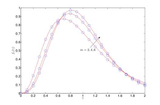
Figure 1: Analytical $-\!\!-$ and simulated $\circ$ PDFs for $\kappa_{l}=2$, $\mu_{l}=2$, $m=2,4,6$, $L=2$, and $\rho_{ij}=0.7^{|i-j|}$.

II-A Sum of I.I.D. Squared $\kappa-\mu$ Shadowed Random Variables

If all squared $\kappa-\mu$ shadowed RVs are independent and identically distributed (i.i.d.), then $\kappa_{l}=\kappa$ and $\mu_{l}=\mu$. From (10)-(18), it can be found that in this case, $\rho_{ij}=\rho_{ji}=0$ and the matrix DC contains uniform eigenvalues, $\lambda_{l}=\kappa\mu/m$; hence, $\delta_{k}=0$, $\forall k>0$. After substituting these values in (21), we get the PDF of sum of i.i.d. squared $\kappa-\mu$ shadowed RVs:

$$f_{\gamma}(\gamma)=\left(\frac{L\mu(1+\kappa)}{\bar{\gamma}}\right)^{L\mu}\left(\frac{m}{m+\kappa\mu}\right)^{Lm}\frac{\gamma^{L\mu-1}}{\Gamma(L\mu)}$$

$$\times e^{-\frac{L\mu(1+\kappa)}{\bar{\gamma}}\gamma}{}_{1}F_{1}\left(Lm;L\mu;\frac{L\kappa\mu^{2}(1+\kappa)\gamma}{\bar{\gamma}(m+\kappa\mu)}\right).$$ (23)

It can be easily verified from (23) that for $L=1$, we get the PDF of the square of a single $\kappa-\mu$ shadowed RV which matches with the PDF given in [8, Eq. (4)].

III Performance Analysis of the MRC Diversity System

III-A System and Channel Model

Consider an $L$-branch MRC at the receiver, where each branch experiences the correlated $\kappa-\mu$ shadowed fading with an instantaneous SNR $\gamma_{l}$, $l=1,..,L$; the correlation coefficient is given in (10). The received instantaneous SNR of the MRC receiver, i.e., $\gamma=\sum^{L}_{l=1}\gamma_{l}$ is characterized in (21).

III-B Moment Generating Function of the Received SNR

The MGF of the received SNR is expressed as

$$M_{\gamma}(s)=E_{\gamma}[e^{-s\gamma}].$$ (24)

From (21) and (24), the MGF of the SNR will be

$$M_{\gamma}(s)=A\left(\frac{\eta}{\bar{\gamma}}\right)^{\epsilon}\sum^{\infty}_{k=0}\tilde{D}_{k}$$

$$\times\int^{\infty}_{0}\gamma^{{\epsilon-1}}e^{-\left(s+\frac{\eta}{\bar{\gamma}}\right)\gamma}{}_{1}F_{1}\big{(}Lm+k;\epsilon;\frac{\eta\gamma}{\bar{\gamma}\left(1+\frac{1}{\lambda_{1}}\right)}\Big{)}d\gamma.$$ (25)

The following relations can be employed in (25):

$${}_{1}F_{1}\Big{(}Lm+k;\epsilon;\frac{\eta\gamma}{\bar{\gamma}\left(1+\frac{1}{\lambda_{1}}\right)}\Big{)}$$

$$=\frac{\Gamma\left(\epsilon\right)}{\Gamma\left(Lm+k\right)}G^{11}_{12}\Bigg{(}-\frac{\eta\gamma}{\bar{\gamma}\left(1+\frac{1}{\lambda_{1}}\right)}\Bigg{|}{1-Lm-k\atop{0,1-\epsilon}}\Bigg{)}$$ (26)

and

$$e^{-(s+\frac{\eta}{\bar{\gamma}})\gamma}=G^{10}_{01}\Bigg{(}(s+\frac{\eta}{\bar{\gamma}})\gamma\Bigg{|}{.\atop{0}}\Bigg{)},$$ (27)

where $G_{p,q}^{m,n}(\cdot|{\cdots\atop\cdots})$ is the Meijer-G function [15, Eq. (9.301)]. After substitution of these relations, we get

$$M_{\gamma}(s)=A\left(\frac{\eta}{\bar{\gamma}}\right)^{\epsilon}\sum^{\infty}_{k=0}\tilde{D}_{k}\frac{\Gamma\left(\epsilon\right)}{\Gamma\left(Lm+k\right)}\int^{\infty}_{0}\gamma^{{\epsilon-1}}$$

$$\times G^{10}_{01}\Bigg{(}\!\!(s+\frac{\eta}{\bar{\gamma}})\gamma\Bigg{|}{.\atop{0}}\!\!\Bigg{)}G^{11}_{12}\Bigg{(}\!\!\frac{-\eta\gamma}{\bar{\gamma}\left(1+\frac{1}{\lambda_{1}}\right)}\Bigg{|}{1-Lm-k\atop{0,1-\epsilon}}\!\!\Bigg{)}d\gamma.$$ (28)

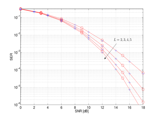
Figure 2: Analytical $-\circ-$ and simulated $+$ SERs for $\kappa_{l}=5$, $\mu_{l}=2$, $m=2$, $\rho_{ij}=0.5^{|i-j|}$, $L=2,3,4,5$, and QPSK constellation.

The integral in (28) can be solved by using [16, Eq. (21)] and we get

$$M_{\gamma}(s)=A\left(\frac{\eta}{\bar{\gamma}}\right)^{\epsilon}\sum^{\infty}_{k=0}\tilde{D}_{k}\frac{\Gamma\left(\epsilon\right)}{\Gamma\left(Lm+k\right)}\left(s+\frac{\eta}{\bar{\gamma}}\right)^{-\epsilon}$$

$$\times G^{12}_{22}\Bigg{(}\frac{-\eta}{\bar{\gamma}\left(1+\frac{1}{\lambda_{1}}\right)\left(s+\frac{\eta}{\bar{\gamma}}\right)}\Bigg{|}{1-Lm-k,1-\epsilon\atop{0,1-\epsilon}}\Bigg{)}.$$ (29)

The MGF for i.i.d. case can be easily calculated by using (23) and method given above. Alternatively, the MGF for i.i.d. case can also be obtained from (29) by putting $\delta_{0}=1$, $\delta_{k}=0$, $k>0$, $\lambda_{l}=\kappa\mu/m$, $\epsilon=L\mu$, and $\eta=L\mu(1+\kappa)$.

The SER of the scheme for $M$-PSK constellation can be efficiently calculated by employing the following relation [17, Eq. (10)]:

$$P_{MPSK}\approx\sum^{3}_{p=1}\beta_{p}M_{\gamma}\left(\alpha_{p}\right),$$ (30)

where $\beta_{1}=\theta_{M}/(2\pi)-1/6$, $\beta_{2}=1/4$, $\beta_{3}=\theta_{M}/(2\pi)-1/4$, $\alpha_{1}=g_{MPSK}$, $\alpha_{2}=4g_{MPSK}/3$, $\alpha_{3}=g_{MPSK}/sin^{2}(\theta_{M})$, $g_{MPSK}=sin^{2}(\pi/M)$, and $\theta_{M}=(M-1)\pi/M$.

The analytical SER for $\kappa_{l}=5$, $\mu_{l}=2$, $m=2$, $\rho_{ij}=0.5^{|i-j|}$, $L=2,3,4,5$, and QPSK constellation is plotted in Fig. 2. The simulated SER versus SNR plots are also shown for the same parameters in the figure. The simulated SER values are obtained by using $10^{7}$ channel realizations. The simulated SER closely follows the analytical SER values at all SNR values considered in the figure. Further, the performance of the MRC receiver improves with increasing value of antennas, as seen from the figure.

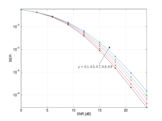
Figure 3: Analytical SER versus SNR plots for $\kappa_{l}=5$, $\mu_{l}=2$, $m=2.5$, $\rho_{ij}=\rho^{|i-j|}$, $\rho=0.1,0.5,0.7,0.8,0.9$, $L=3$, and QPSK constellation.

The effect of correlation parameter $\rho$ on the SER performance of the MRC receiver is shown in Fig. 3 for $\kappa_{l}=5$, $\mu_{l}=2$, $m=2.5$, $\rho_{ij}=\rho^{|i-j|}$, $\rho=0.1,0.5,0.7,0.8,0.9$, $L=3$, and QPSK constellation. It can be seen from the figure that the receiver error performance degrades with increasing value of the correlation coefficient.

III-C Diversity Order Calculation

By using the Slater’s theorem [18, Eq. (8.2.2.3)] which represents the Meijer-G function as a finite series of the Hypergeometric function, it can be shown that

$$G^{12}_{22}\Bigg{(}\frac{-\eta}{\bar{\gamma}\left(1+\frac{1}{\lambda_{1}}\right)\left(s+\frac{\eta}{\bar{\gamma}}\right)}\Bigg{|}{1-Lm-k,1-\epsilon\atop{0,1-\epsilon}}\Bigg{)}$$

$$=\Gamma(Lm+k){}_{2}F_{1}\!\!\!\left(Lm+k,\epsilon;\epsilon;\frac{\eta\left(s+\frac{\eta}{\bar{\gamma}}\right)^{-1}}{\bar{\gamma}\left(1+\frac{1}{\lambda_{1}}\right)}\right),$$ (31)

where ${{}_{2}F_{1}(a_{1},a_{2};b_{1};z)}$ is the Gaussian Hypergeometric function [15]. From (29) and (31), the MGF of the MRC scheme can be written as

$$M_{\gamma}(s)=A\left(\frac{\eta}{\bar{\gamma}}\right)^{\epsilon}\sum^{\infty}_{k=0}\tilde{D}_{k}{\Gamma\left(\epsilon\right)}\left(s+\frac{\eta}{\bar{\gamma}}\right)^{-\epsilon}$$

$$\times{}_{2}F_{1}\left(Lm+k,\epsilon;\epsilon;\frac{\eta}{\bar{\gamma}\left(1+\frac{1}{\lambda_{1}}\right)\left(s+\frac{\eta}{\bar{\gamma}}\right)}\right).$$ (32)

For diversity calculation, let us assume that $\bar{\gamma}$ is very large, which means that ${\eta}/\left({\bar{\gamma}\left(1+\frac{1}{\lambda_{1}}\right)\left(s+\frac{\eta}{\bar{\gamma}}\right)}\right)$ is very small. Therefore, after observing the fact that ${{}_{2}F_{1}(a_{1},a_{2};b_{1};z)}\rightarrow 1$, $z\rightarrow 0$ [19] and after some other algebra, the asymptotic value of the MGF is given by

$$M_{\gamma}(s)=A\left(\frac{\eta}{\bar{\gamma}}\right)^{\epsilon}\sum^{\infty}_{k=0}\tilde{D}_{k}{\Gamma\left(\epsilon\right)}s^{-\epsilon}.$$ (33)

The diversity order of the MRC scheme is $\epsilon=\sum^{L}_{l=1}\mu_{l}$, as seen from (33).

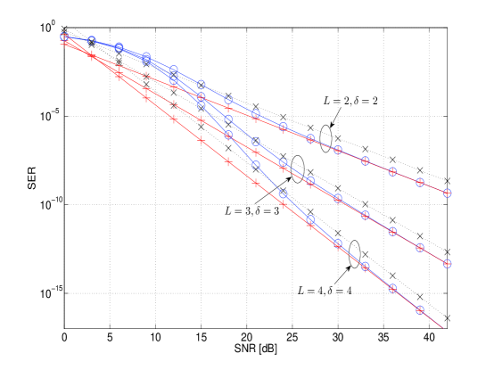
Figure 4: Analytical $-\circ-$ and asymptotic $-+-$ SERs for $\kappa_{l}=10$, $\mu_{l}=1$, $m=3$, $\rho_{ij}=0.1^{|i-j|}$, $L=2,3,4$, and QPSK constellation; the asymptotic ideal diversity plots are shown by $-\times-$.

For verifying the analytical diversity order, we have plotted the asymptotic SER by using (30) and (33) in Fig. 4. The analytical SER versus SNR plots (obtained from (29) and (30)) are also shown in the figure. All plots are given for $\kappa_{l}=10$, $\mu_{l}=1$, $m=3$, $\rho_{ij}=0.1^{|i-j|}$, $L=2,3,4$, and QPSK constellation. It can be seen from the figure that the asymptotic SER closely overlaps with the analytical SER at high values of the SNR. Therefore, the proposed asymptotic MGF in (33) is sufficiently tight at high SNR. Further, we have also plotted the asymptotic ideal diversity curves by using the relation: $\alpha/\bar{\gamma}^{\delta}$, where $\alpha$ is a positive real coefficient and $\delta$ denotes the ideal diversity. The SER versus SNR performance of the MRC receiver decays at the same rate as that of the slope of the asymptotic ideal diversity curves in all cases. The correctness of the diversity analysis is corroborated from the figure.

III-D Average BER Calculation

By using the series representation of the confluent Hypergeometric function:

$${}_{1}F_{1}(a;b;x)=\sum^{\infty}_{n=0}\frac{(a)_{n}}{(b)_{n}n!}x^{n},$$ (34)

where $(\cdot)_{n}$ is the Pochhammer symbol, in (21), we get

$$f_{\gamma}(\gamma)=A\left(\frac{\eta}{\bar{\gamma}}\right)^{\epsilon}\sum^{\infty}_{k=0}\tilde{D}_{k}\sum^{\infty}_{j=0}C_{j,k}\gamma^{j+\epsilon-1}e^{-\frac{\eta}{\bar{\gamma}}\gamma},$$ (35)

where

$$C_{j,k}=\frac{(Lm+k)_{j}}{(\epsilon)_{j}j!}\left(\frac{\eta}{\bar{\gamma}\left(1+\frac{1}{\lambda_{1}}\right)}\right)^{j}.$$ (36)

From the signal-space concept, the average BER of $M$-PSK/QAM constellation is given by [20, 21, 22, 7]

$$Pe(\gamma)=\zeta_{M}\sum^{\tau_{M}}_{p=1}Q\left(a_{p}\sqrt{\gamma}\right),$$ (37)

where $Q(\cdot)$ is the q-function [10, Eq. (2.1.97)], $\zeta_{M}$, $a_{p}$, and $\tau_{M}$ are modulation dependent parameters, given in Table I. The average BER of the considered scheme will be

$$Pe(\bar{\gamma})=A\zeta_{M}\left(\frac{\eta}{\bar{\gamma}}\right)^{\epsilon}\sum^{\infty}_{k=0}\tilde{D}_{k}\sum^{\infty}_{j=0}C_{j,k}$$

$$\times\sum^{\tau_{M}}_{p=1}\int^{\infty}_{0}\gamma^{j+\epsilon-1}e^{-\frac{\eta}{\bar{\gamma}}\gamma}Q\left(a_{p}\sqrt{\gamma}\right)d\gamma.$$ (38)

TABLE I: Values of $\zeta_{M}$, $\tau_{M}$, and $a_{p}$ for different constellations.

Constellation	$\zeta_{M}$	$\tau_{M}$	$a_{p}$
$M$-QAM	$\frac{4\left(1-\frac{1}{\sqrt{M}}\right)}{\log_{2}M}$	$\frac{\sqrt{M}}{2}$	$\left(2p-1\right)\sqrt{\frac{3}{(M-1)}}$
$M$-PSK	$\frac{2}{\max\left(\log_{2}M,2\right)}$	$\max\left(\frac{M}{4},1\right)$	$\sqrt{2}\sin\frac{(2k-1)\pi}{M}$

By using the relation $Q\left(a_{p}\sqrt{\gamma}\right)=(1/2)\mbox{erfc}(a_{p}\sqrt{\gamma}/\sqrt{2})$ and [14, Eq. (2.8.5.7)] in (38), we get the average BER of the scheme as

$$Pe(\bar{\gamma})=A\zeta_{M}\left(\frac{\eta}{\bar{\gamma}}\right)^{\epsilon}\sum^{\infty}_{k=0}\tilde{D}_{k}\sum^{\infty}_{j=0}C_{j,k}$$

$$\times\sum^{\tau_{M}}_{p=1}\frac{\left(a_{p}/\sqrt{2}\right)^{-2\epsilon-2j}}{(2\epsilon+2j)\sqrt{\pi}}\Gamma(\epsilon+j+1/2)$$

$$\times{}_{2}F_{1}\left(\epsilon+j,\epsilon+j+1/2;\epsilon+j+1;-\frac{2\eta}{a^{2}_{p}\bar{\gamma}}\right).$$ (39)

By employing the relation: ${}_{2}F_{1}\left(\epsilon+j,\epsilon+j+1/2;\epsilon+j+1;-\frac{2\eta}{a^{2}_{p}\bar{\gamma}}\right)=1$ for very high value of $\bar{\gamma}$ in (39), we get

$$Pe(\bar{\gamma})=A\zeta_{M}\left(\frac{\eta}{\bar{\gamma}}\right)^{\epsilon}\sum^{\infty}_{k=0}\tilde{D}_{k}\sum^{\infty}_{j=0}C_{j,k}$$

$$\times\sum^{\tau_{M}}_{p=1}\frac{\left(a_{p}/\sqrt{2}\right)^{-2\epsilon-2j}}{(2\epsilon+2j)\sqrt{\pi}}\Gamma(\epsilon+j+1/2).$$ (40)

It can be seen from (36) that $C_{j,k}$ varies inversely with $\bar{\gamma}^{j}$. Therefore, for the diversity calculation, we should set $j=0$. By setting $j=0$ and $p=1$ in (40), we get the asymptotic BER of the scheme:

$$Pe(\bar{\gamma})=\frac{A\zeta_{M}\Gamma(\epsilon+1/2)}{2\epsilon\sqrt{\pi}\left(a_{1}/\sqrt{2}\right)^{2\epsilon}}\left(\sum^{\infty}_{k=0}\tilde{D}_{k}\right)\left(\frac{\eta}{\bar{\gamma}}\right)^{\epsilon}.$$ (41)

It is confirmed from (41) that the diversity order of the MRC receiver is $\epsilon$, as shown in Subsection III.C.

Under the condition that $m$ being an integer and $Lm+k>\epsilon$, the Hypergeometric function in (21) can be represented in the form of a finite series by using the Kummer’s transform [19] as

$${}_{1}F_{1}\big{(}Lm+k;\epsilon;\frac{\eta\gamma}{\bar{\gamma}\left(1+\frac{1}{\lambda_{1}}\right)}\Big{)}=e^{\frac{\eta\gamma}{\bar{\gamma}}\left(1+\frac{1}{\lambda_{1}}\right)^{-1}}$$

$$\times\sum^{Lm+k-\epsilon}_{j=0}\frac{(Lm+k-\epsilon)!}{(Lm-\epsilon-j)!j!(\epsilon)_{j}}\left(\frac{\eta\gamma}{\bar{\gamma}\left(1+\frac{1}{\lambda_{1}}\right)}\right)^{j}.$$ (42)

Using (42), the BER can be calculated in the form of a single power series employing the method stated before.

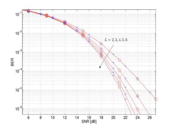
Figure 5: Analytical $-\circ-$ and simulated $+$ BERs for $\kappa_{l}=2$, $\mu_{l}=2$, $m=2.1$, $\rho_{ij}=0.2^{|i-j|}$, $L=2,3,4,5,6$, and 16-QAM constellation.

The analytical and simulated BER versus SNR plots for $\kappa_{l}=2$, $\mu_{l}=2$, $m=2.1$, $\rho_{ij}=0.2^{|i-j|}$, $L=2,3,4,5,6$, and 16-QAM constellation are shown in Fig. 5. The simulated BER values are obtained by using $10^{7}$ channel realizations. The closeness of the analytical and simulated BER plots is evident from the figure. Moreover, the performance of the MRC scheme is improved with increasing value of receive antennas, as seen from Fig. 5.

III-E Ergodic Capacity Analysis

The average capacity (in bits/sec/Hz) of the scheme is given by

$$C(\bar{\gamma})=\int^{\infty}_{0}\mbox{log}_{2}\left(1+\gamma\right)f_{\gamma}(\gamma)d\gamma.$$ (43)

By using the relations:

$$e^{-\frac{\eta}{\bar{\gamma}}\gamma}=G^{10}_{01}\Bigg{(}\frac{\eta}{\bar{\gamma}}\gamma\Bigg{|}{.\atop{0}}\Bigg{)}$$ (44)

and

$$\mbox{ln}\left(1+\gamma\right)=G^{12}_{22}\Bigg{(}\gamma\Bigg{|}{1,1\atop{1,0}}\Bigg{)},$$ (45)

where $\mbox{ln}(\cdot)$ is the natural logarithm, and (27) and (35), in (43), we get

$$C(\bar{\gamma})=\frac{A}{\mbox{ln}2}\left(\frac{\eta}{\bar{\gamma}}\right)^{\epsilon}\sum^{\infty}_{k=0}\tilde{D}_{k}\sum^{\infty}_{j=0}C_{j,k}$$

$$\times\int^{\infty}_{0}\gamma^{j+\epsilon-1}G^{10}_{01}\Bigg{(}\frac{\eta}{\bar{\gamma}}\gamma\Bigg{|}{.\atop{0}}\Bigg{)}G^{12}_{22}\Bigg{(}\gamma\Bigg{|}{1,1\atop{1,0}}\Bigg{)}d\gamma.$$ (46)

Employing [16, Eq. (21)] in (46), we have

$$C(\bar{\gamma})=\frac{A}{\mbox{ln}2}\sum^{\infty}_{k=0}\tilde{D}_{k}\sum^{\infty}_{j=0}C_{j,k}\left(\frac{\eta}{\bar{\gamma}}\right)^{-j}$$

$$\hskip 30.00005pt\times G^{13}_{32}\Bigg{(}\frac{\bar{\gamma}}{\eta}\Bigg{|}{1,1,1-\epsilon-j\atop{1,0}}\Bigg{)}.$$ (47)

In Fig. 6, the analytical average capacity of the MRC scheme is plotted for $\kappa_{l}=2$, $\mu_{l}=2$, $m=1.2$, $\rho_{ij}=0.5^{|i-j|}$, and $L=2,3$ by using (47). Moreover, the plots of the capacity obtained by numerical integration of (43) are provided in the figure to verify the validity of the proposed capacity results of (47). It can be seen from the figure that there is a significant improvement in the average capacity of the correlated $\kappa-\mu$ shadowed channels with increasing number of the spatial dimension. For example, at SNR=10 dB there is 30% increment in the average capacity by using three antennas as compared to the two antennas case.

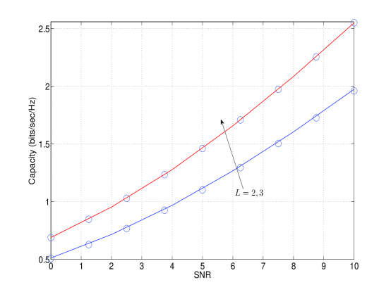
Figure 6: Capacity plots for $\kappa_{l}=2$, $\mu_{l}=2$, $m=1.2$, $\rho_{ij}=0.5^{|i-j|}$, and $L=2,3$ obtained by using (47) $-\!\!-$ and (43) $\circ$ .

IV Conclusions

We have statistically characterized the correlated $\kappa-\mu$ shadowed fading in this paper, in terms of PDF and MGF. These characterizations have been found useful for study of the error performance and diversity performance of the MRC scheme. The analytical results have been obtained in terms of power series of the Hypergeometric functions and Meijer-G function. A study of the LOS correlation on the error performance of the MRC receiver has been performed by using the derived analytical results. It has been deduced on the basis of the analytical results that the error performance of the receiver is adversely affected by the antenna correlation. However, the diversity order of the MRC scheme remains independent of the antenna correlation.

References

- [1] M. D. Yacoub, “The and the distribution,” IEEE Antennas and Propagation Magazine, vol. 49, pp. 68–81, Feb. 2007.
- [2] A. Abdi, W. Lau, M.-S. Alouini, and M. Kaveh, “A new simple model for land mobile satellite channels: First and second order statistics,” IEEE Trans. Wireless Commun., vol. 2, no. 3, pp. 519–528, May 2003.
- [3] M. R. Bhatnagar and Arti M.K., “Performance analysis of AF based hybrid satellite-terrestrial cooperative network over generalized fading channels,” IEEE Commun. Lett., vol. 17, no. 10, pp. 1912–1915, Oct. 2013.
- [4] Arti M.K. and M. R. Bhatnagar, “Beamforming and combining in hybrid satellite-terrestrial cooperative systems,” IEEE Commun. Lett., vol. 18, no. 3, pp. 483–486, March 2014.
- [5] M. R. Bhatnagar and Arti M.K., “Performance analysis of hybrid satellite-terrestrial FSO cooperative system,” IEEE Photon. Technol. Lett., vol. 25, no. 22, pp. 2197–2200, Nov. 2013.
- [6] Arti M.K. and M. R. Bhatnagar, “Two-way mobile satellite relaying: A beamforming and combining based approach,” IEEE Commun. Lett., vol. 18, no. 7, pp. 1187–1190, July 2014.
- [7] M. R. Bhatnagar and Arti M.K., “On the closed-form performance analysis of maximal ratio combining in Shadowed-Rician fading LMS channels,” IEEE Commun. Lett., vol. 18, no. 1, pp. 54–57, Jan. 2014.
- [8] J. F. Paris, “Statistical characterization of shadowed fading,” IEEE Trans. Vehicular Technol., vol. 63, no. 2, pp. 518 – 526, Feb. 2014.
- [9] G. Alfano and A. D. Maio, “Sum of squared Shadowed-Rice random variables and its application to communication systems performance prediction,” IEEE Trans. Wireless Commun., vol. 6, no. 10, pp. 3540–3545, Oct. 2007.
- [10] J. G. Proakis, Digital Communications, 4th ed. Singapore: McGraw-Hill, 2001.
- [11] M.-S. Alouini, A. Abdi, and M. Kaveh, “Sum of Gamma variates and performance of wireless communication systems over Nakagami-fading channels,” IEEE Trans. Vehicular Technol., vol. 50, no. 6, pp. 1471 – 1480, Nov. 2001.
- [12] P. G. Moschopoulos, “The distribution of the sum of independent Gamma random variables,” Ann. Inst. Statist. Math. (Part A), vol. 37, pp. 541–544, 1985.
- [13] Y. Dhungana, N. Rajatheva, and C. Tellambura, “Performance analysis of antenna correlation on LMS-based dual-hop AF MIMO systems,” IEEE Trans. Vehicular Technol., vol. 61, no. 8, pp. 3590–3602, Oct. 2012.
- [14] A. P. Prudnikov, Y. A. Brychkov, and O. I. Marichev, Integrals and Series, 3rd ed. New York, USA: Gordon and Breach Science Publishers, 1992, vol. 2.
- [15] I. S. Gradshteyn and I. M. Ryzhik, Table of Integrals, Series, and Products, 6th ed. San Diego, CA, USA: Academic Press, 2000.
- [16] V. S. Adamchik and O. Marichev, “The algorithm for calculating integrals of hypergeometric type function and its realization in reduce system,” in Proc. International Symposium on Symbolic Algebraic Computation (ISSAC’90), Tokyo, Japan, Aug. 1990, pp. 212–224.
- [17] M. McKay, A. Zanella, I. Collings, and M. Chiani, “Error probability and SINR analysis of optimum combining in Rician fading,” IEEE Trans. Commun., vol. 57, no. 3, pp. 676–687, March 2009.
- [18] A. P. Prudnikov, Y. A. Brychkov, and O. I. Marichev, Integrals and Series, 1st ed. New York, USA: Gordon and Breach Science Publishers, 1990, vol. 3.
- [19] M. Abramowitz and I. A. Stegun, Handbook of Mathematical Functions. New York, USA: Dover Publications, Inc., 1972.
- [20] J. Lu, K. B. Letaief, J. C.-I. Chuang, and M. L. Liou, “-PSK and -QAM BER computation using signal-space concepts,” IEEE Trans. Commun., vol. 47, no. 2, pp. 181–184, Feb. 1999.
- [21] M. R. Bhatnagar, “Performance analysis of a path selection scheme in multi-hop decode-and-forward protocol,” IEEE Commun. Lett., vol. 16, no. 12, pp. 1980–1983, Dec. 2012.
- [22] Arti M.K. and M. R. Bhatnagar, “Performance analysis of hop-by-hop beamforming and combining in DF MIMO relay system over Nakagami- fading channels,” IEEE Commun. Lett., vol. 17, no. 11, pp. 2080–2083, Nov. 2013.