IST versus PDE, a comparative study

Abstract

We survey and compare, mainly in the two-dimensional case, various results obtained by IST and PDE techniques for integrable equations. We also comment on what can be predicted from integrable equations on non integrable ones.

To Walter Craig with friendship and admiration

1 Introduction

The theory of nonlinear dispersive equations has been flourishing during the last thirty years. Partial differential equations (PDE) techniques (in the large) have led to striking results concerning the resolution of the Cauchy problem, blow-up issues, stability analysis of various "localized" solutions. On the other hand, a few nonlinear dispersive equations or systems are integrable by Inverse Scattering Transform (IST) techniques. This allows a deep understanding of the equation dynamic and also to make relevant conjectures on close, non integrable equations. The best example is the Korteweg-de Vries (KdV) equation for which IST allows to prove that any solution to the Cauchy problem with sufficiently smooth and decaying initial data decomposes into a finite train of solitons traveling to the right and a dispersive tail traveling to the left (see Schu and the references therein and section 1).

The aim of the present paper is to survey and compare, on specific examples, the advantages and shortcomings of PDE and IST techniques and also how they can benefit from each other. We will restrain to the Cauchy problem posed on the whole space $\mathbb{R}$ or $\mathbb{R}^{2}$ since the corresponding periodic problems lead to rather different issues, both by the two approaches.

The paper will be organized as follows. The first section is devoted to one-dimensional (spatial) problems. After recalling the KdV case for which the IST techniques yield the more complete results and which can be seen as a paradigm of what is expected for "close", possibly not integrable equations, we then consider two nonlocal integrable equations, the Benjamin-Ono (BO) and Intermediate Long Wave (ILW) equations that have a much less complete IST theory than the KdV equation. We will in this section present some numerical simulations from KS showing that the long time dynamics of KdV solutions seems to be inherited by those of some non integrable equations, such as the fractional KdV or BBM equations. We close this Section by the one-dimensional Gross-Pitaevskii equation, a defocusing nonlinear Schrödinger equation for which non trivial boundary conditions at infinity provide some focusing behavior. At this example, one can compare, for the specific problem of the stability of the black soliton, the differences between the two methods. We will provide here some details since this example might be less known than for instance the KdV equation.

We then turn to two-dimensional equations. Section two is devoted to the Kadomtsev-Petviashvili equations (KP). Finally, the last section deals with the family of Davey-Stewartson systems, two members of which are integrable (the so-called DSI and DS II system). An important issue is whether or not some of the remarkable properties of the integrable DS systems persist in the non integrable case.

We conclude by a short mention of two other integrable two-dimensional systems, the Ishimori and the Novikov-Veselov systems.

2 Notations

The following notations will be used throughout this article. The partial derivative will be denoted by $u_{x},...$ or $\partial_{x}\phi,..$. For any $s\in\mathbb{R},$ $D^{s}=(-\Delta)^{\frac{s}{2}}$ and $J^{s}=(I-\Delta)^{\frac{s}{2}}$ denote the Riesz and Bessel potentials of order $-s$, respectively.

The Fourier transform of a function $f$ is denoted by $\hat{f}$ or $\mathcal{F}(f)$ and the dual variable of $x\in\mathbb{R}^{d}$ is denoted $\xi.$ For $1\leq p\leq\infty$, $L^{p}(\mathbb{R})$ is the usual Lebesgue space with the norm $|\cdot|_{p}$, and for $s\in\mathbb{R}$, the Sobolev spaces $H^{s}(\mathbb{R}^{2})$ are defined via the usual norm $\|\phi\|_{s}=|J^{s}\phi|_{2}$.

$\mathcal{S}(\mathbb{R}^{d})$ will denote the Schwartz space of smooth rapidly decaying functions in $\mathbb{R}^{d}$, and $\mathcal{S}^{\prime}(\mathbb{R}^{d})$ the space of tempered distributions.

3 The one-dimensional case

3.1 The KdV equation

The KdV equation is historically the first nonlinear dispersive equation which has been written down. It was in fact derived formally by Boussinesq (1877). We refer to Da for a complete historical account. The full rigorous derivation from the water wave system is due to W. Craig Craig . We refer to Da for historical aspects and to La for the systematic rigorous derivation of water waves models in various regimes. The KdV equation is (as in fact most of the classical nonlinear dispersive equations or systems) a "universal" asymptotic equation describing a specific dynamic (in the long wave, weakly nonlinear regime) of a large class of complex nonlinear dispersive systems.

The KdV equation

$$u_{t}-6uu_{x}+u_{xxx}=0,$$ (1)

is also the first nonlinear PDE for which the Inverse scattering technique was successively applied (see for instance GGKM ; Lax ).

It is associated to the spectral problem for the Schrödinger operator

$$L(t)=-\frac{d^{2}\psi}{dx^{2}}+u(\cdot,t)\psi$$

considered as an unbounded operator in $L^{2}(\mathbb{R}).$

We thus consider the spectral problem

$$\psi_{xx}+(k^{2}-u(x,t))\psi=0,\quad-\infty<x<+\infty.$$

Given $u_{0}=u(\cdot,0)$ sufficiently smooth and decaying at $\pm\infty,$ say in the Schwartz space $\mathcal{S}(\mathbb{R}),$ one associates to $L(0)$ its spectral data, that is a finite (possibly empty) set of negative eigenvalues $-\kappa_{1}^{2}<-\kappa^{2}_{2}\cdot\cdot\cdot<-\kappa_{N}^{2},$ together with right normalization coefficients $c_{j}^{r}$ and right reflection coefficients $b_{r}(k)$ (see Schu for precise definitions and properties of those objects).

The spectral data consists thus in the collection of $\{b_{r}(k),\kappa_{j},c_{j}^{r}\}.$ It turns out that if $u(x,t)$ evolves according to the KdV equation, the scattering data evolves in a very simple way:

$$\kappa_{j}(t)=\kappa_{j},$$

$$c_{j}^{r}(t)=c_{j}^{r}\exp(4\kappa_{j}^{3}t),\quad j=1,2,\cdot\cdot\cdot,N,$$

$$b_{r}(k,t)=b_{r}(k)\exp(8ik^{3}t),\quad-\infty<k<+\infty.$$

The potential $u(x,t)$ is recovered as follows. Let

$$\Omega(\xi;t)=2\sum_{j=1}^{N}[c^{r}_{j}(t)]^{2}e^{-2\kappa_{j}\xi}+\frac{1}{\pi}\int_{-\infty}^{\infty}b_{r}(k,t)e^{2ik\xi}dk.$$

One then solves the linear integral equation (Gel’fand-Levitan- Marchenko equation):

$$\beta(y;x,t)+\Omega(x+y;t)+\int_{0}^{\infty}\Omega(x+y+z;t)\beta(z;x,t)dz=0,\quad y>0,\;x\in\mathbb{R},\;t>0.$$ (2)

The solution of the Cauchy problem (60) is then given by

$$u(x,t)=-\frac{\partial}{\partial x}\beta(0^{+};x,t),\quad x\in\mathbb{R},\quad t>0.$$

One obtains explicit solutions when $b_{r}=0.$ A striking case is obtained when the scattering data are $\{0,\kappa_{j},c_{j}^{r}(t)\}.$ This corresponds to the so-called $N-soliton$ solution $u_{d}(x,t)$ according to its asymptotic behavior obtained by Tanaka Tana :

$$\lim_{t\to\infty}\;\sup_{x\in\mathbb{R}}\left|u_{d}(x,t)-\sum_{p=1}^{N}\left(-2\kappa_{p}^{2}\text{sech}^{2}[\kappa_{p}(x-x_{p}^{+}-4\kappa_{p}^{2}t)]\right)\right|=0,$$ (3)

where

$$x_{p}^{+}=\frac{1}{2\kappa_{p}}\log\left\{\frac{\left[c_{p}^{r}\right]^{2}}{2\kappa_{p}}\prod_{l=1}^{p-1}\left(\frac{\kappa_{l}-\kappa_{p}}{\kappa_{l}+\kappa_{p}}\right)^{2}\right\}.$$

In other words, $u_{d}(x,t)$ appears for large positive time as a sequence of $N$ solitons, with the largest one in the front, uniformly with respect to $x\in\mathbb{R}.$

For $u_{0}\in\mathcal{S}(\mathbb{R})$, the solution of (60) has the following asymptotics

$$\sup_{x\geq-t^{1/3}}|u(x,t)|=O(t^{-2/3}),\quad\text{as}\;t\to\infty,$$ (4)

in the absence of solitons (that is when $L(0)$ has no negative eigenvalues) and

$$\sup_{x\geq-t^{1/3}}|u(x,t)-u_{d}(x,t)|=O(t^{-1/3}),\quad\text{as}\;t\to\infty$$ (5)

in the general case, the $N$ in $u_{d}$ being the number of negative eigenvalues of $L(0).$ One has moreover the convergence result

$$\lim_{t\to+\infty}\;\sup_{x\geq-t^{1/3}}\left|u(x,t)-\sum_{p=1}^{N}\left(-2\kappa_{p}^{2}\text{sech}^{2}[\kappa_{p}(x-x_{p}^{+}-4\kappa_{p}^{2}t)]\right)\right|=0.$$ (6)

In both cases, a "dispersive tail" propagates to the left.

Remark 1

The shortcoming of those remarkable results is of course that they apply only to the integrable KdV equation and also to the modified KdV equation

$$u_{t}+6u^{2}u_{x}+u_{xxx}=0.$$

However, though they are out of reach of "classical" PDE methods, they give hints on the behavior of other, non integrable, equations whose dynamics could be in some sense similar.

Remark 2

As previously noticed, the results obtained by IST methods necessitate a decay property of the initial data, the minimal condition being

$$I(0)=\int_{-\infty}^{\infty}(1+|x|)|u_{0}(x)|dx<\infty.$$ (7)

This condition ensures in particular (Marc ) that $L(0)$ has a finite number of discrete eigenvalues, more precisely (CaDe ), the number $N$ of eigenvalues of $L(0)$ is bounded by $1+I(0)$.

This excludes for instance initial data in the energy space $H^{1}(\mathbb{R})$ in which the Cauchy problem is globally well-posed (KPV2 ). The global behavior of the flow might thus be different from the aforementioned results for such initial data.

Remark 3

1. Stemming from the seminal work of Bourgain Bourgain , PDE techniques allow to prove the well-posedness of the Cauchy problem for the KdV equation with initial data in very large spaces, namely $H^{s}(\mathbb{R}),s>-\frac{3}{4},$ (see KPV3 ) which includes in particular measures, for instance the Dirac distribution.

2. PDE techniques yield also the asymptotic stability of the solitary waves for subcritical KdV equations with a rather general nonlinearity (MaMe ; MaMe1 ) which can be seen as a first step towards the soliton resolution conjecture, see eg Tao .

In order to see to what extent the long time dynamics of the KdV equation is in some sense generic, we will consider as a toy model the fractional KdV (fKdV) equation

$$u_{t}+uu_{x}-D^{\alpha}u_{x}=0,\quad u(.,0)=u_{0},$$ (8)

where $\widehat{D^{\alpha}f}(\xi)=|\xi|^{\alpha}\hat{f}(\xi),\;\alpha>-1.$

Using the Fourier multiplier operator notation

$$\widehat{Lu}(\xi)=p(\xi)\hat{u}(\xi),\quad p(\xi)=|\xi|^{\alpha},$$

it can be rewritten as

$$u_{t}+uu_{x}-Lu_{x}=0,\quad u(.,0)=u_{0},$$ (9)

When $\alpha=2$ (resp.$1$) (8) reduces to the KdV (resp. Benjamin-Ono) equation. If the symbol $|\xi|^{\alpha}$ is replaced by

$$p(\xi)=\left(\frac{\tanh\xi}{\xi}\right)^{1/2},$$

one gets the so-called Whitham equation (Wh ) that models surface gravity waves in an appropriate regime. This symbol behaves like $|\xi|^{-1/2}$ for large frequencies.

When surface tension is included in the Whitham equation, one gets

$$p(\xi)=(1+\beta|\xi|^{2})^{1/2}\left(\frac{\tanh\xi}{\xi}\right)^{1/2},\quad\beta\geq 0$$

which behaves like $|\xi|^{1/2}$ for large $|\xi|.$

The following quantities are formally conserved by the flow associated to (8),

$$M(u)=\int_{\mathbb{R}}u^{2}(x,t)dx,$$ (10)

and the Hamiltonian

$$H(u)=\int_{\mathbb{R}}\big{(}\frac{1}{2}|D^{\frac{\alpha}{2}}u(x,t)|^{2}-\frac{1}{6}u^{3}(x,t)\big{)}dx.$$ (11)

One notices that the values $\alpha=1/3$ and $\alpha=1/2$ correspond respectively to the so-called energy critical and to the $L^{2}$ critical cases. Actually, equation (8) is invariant under the scaling transformation

$$u_{\lambda}(x,t)=\lambda^{\alpha}u(\lambda x,\lambda^{\alpha+1}t),$$ (12)

for any positive number $\lambda$. A straightforward computation shows that $\|u_{\lambda}\|_{\dot{H}^{s}}=\lambda^{s+\alpha-\frac{1}{2}}\|u_{\lambda}\|_{\dot{H}^{s}}$, and thus the critical index corresponding to (8) is $s_{\alpha}=\frac{1}{2}-\alpha$. Thus, equation (8) is $L^{2}$-critical for $\alpha=\frac{1}{2}$. On the other hand the Hamiltonian does not make sense in the energy space $H^{\alpha/2}(\mathbb{R})$ when $\alpha<\frac{1}{3}$. The numerical simulations in KS suggest that the Cauchy problem (8) has global solutions (for arbitrary large suitably localized and smooth initial data) if and only if $\alpha>1/2.$ This has been rigorously proven when $\alpha\geq 1$ (see FLP1 ; FLP2 ) but is an open problem when $1/2<\alpha<1.$ On the other hand, the local Cauchy problem is for $\alpha>0$ locally well-posed in $H^{s}(\mathbb{R}),s>\frac{3}{2}-\frac{3\alpha}{8},$ (LPS ).

More surprising is the fact that the resolution into solitary waves plus dispersion seems to be still valid when $\alpha>1/2$ as also suggested from the numerical simulations in KS from which we extract the following figures. In Fig. 1, one can see the solution for the fKdV equation in the mass subcritical case $\alpha=0.6$ for the initial data $5\text{sech}^{2}x$.

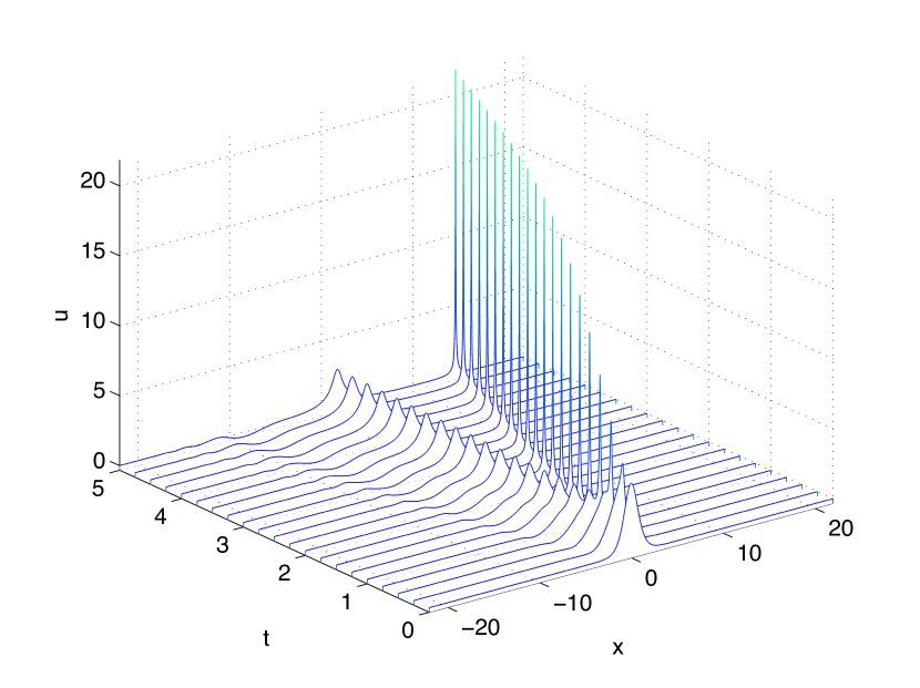
Figure 1: Solution to the fKdV equation (8) for $\alpha=0.6$, for the initial data $\mathfrak{u}_{0}=5\text{sech}^{2}x.$

In Fig. 2 we have fitted the humps with the computed solitary waves. This is an evidence for the above mentioned soliton resolution conjecture.

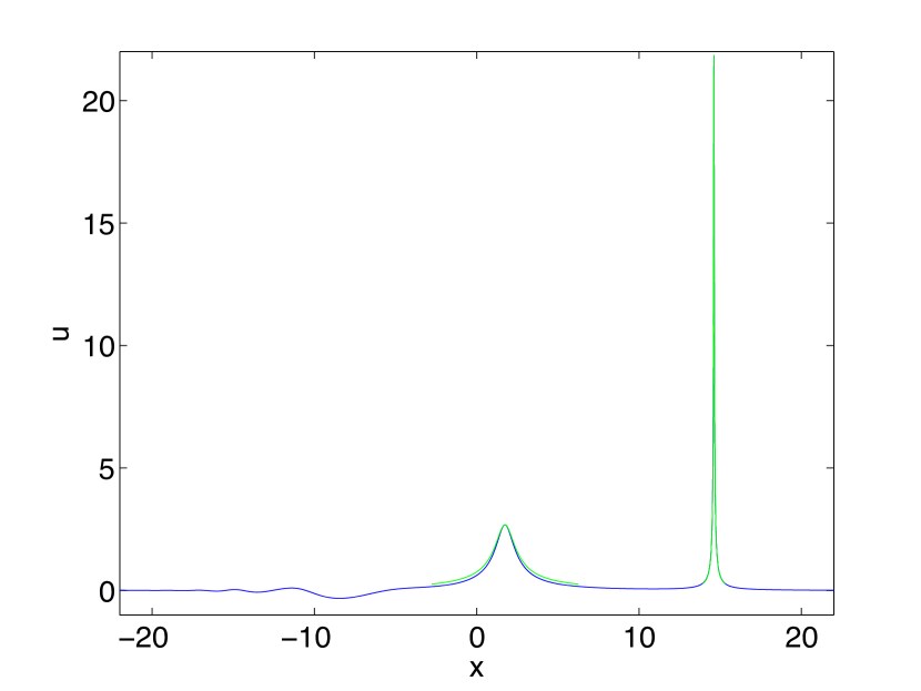
Figure 2: Solution to the fKdV equation (8) for $\alpha=0.6$, and the initial data $\mathfrak{u}_{0}=5\text{sech}^{2}x$ for $t=5$ in blue, fitted solitons at the humps in green.

A similar behavior seems to occur for the fractional BBM equation (fBBM)

$$u_{t}+u_{x}+uu_{x}+D^{\alpha}u_{t}=0$$ (13)

in the subcritical case $\alpha>\frac{1}{3}.$ Again the simulations in KS ) suggest that the soliton resolution also holds (see Figure 3 below).

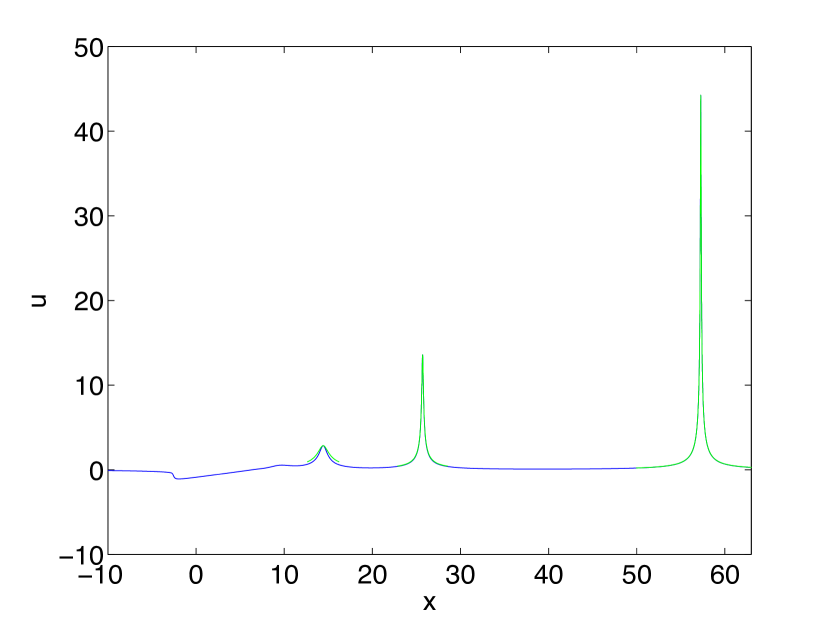
Figure 3: Solution to the fBBM equation (13) for $\alpha=0.5$, and the initial data $\mathfrak{u}_{0}=10\text{sech}^{2}x$ for $t=10$ in blue, fitted solitons at the humps in green.

3.2 The Benjamin-Ono and Intermediate Long Wave Equations

The Intermediate Long Wave Equation (ILW) and the Benjamin-Ono equation (BO) are asymptotic models in an appropriate regime for a two-fluid system when the depth $\delta$ of the bottom layer is very large with respect to the upper one (ILW) or infinite (BO) (see BLS ).

The ILW corresponds (in the notations of ABFS ) to

$$p(\xi)=2\pi\xi\text{coth}\;(2\pi\delta\xi)-\frac{1}{\delta}$$

and the BO equation to

$$p(\xi)=2\pi|\xi|.$$

Alternatively they can be respectively written in convolution form

$$u_{t}+uu_{x}+\frac{1}{\delta}u_{x}+\mathcal{T}_{\delta}(u_{xx})=0,$$ (14)

$$\mathcal{T}_{\delta}(u)(x)=-\frac{1}{2\delta}PV\int_{-\infty}^{\infty}\text{coth}\left(\frac{\pi(x-y)}{2\delta}\right)u(y)dy$$

and

$$u_{t}+uu_{x}+\mathcal{H}u_{xx}=0$$ (15)

where $\mathcal{H}$ is the Hilbert transform

$$\mathcal{H}u(x)=\frac{1}{\pi}PV\int_{-\infty}^{\infty}\frac{u(y)}{x-y}dy.$$

The Benjamin-Ono equation

A striking difference between KdV and BO equations is that the latter is quasilinear rather that semilinear. This means that the Cauchy problem for BO cannot be solved by a Picard iterative scheme implemented on the integral Duhamel formulation, for initial data in any Sobolev spaces $H^{s}(\mathbb{R})$, $s\in\mathbb{R}$. Alternatively, this implies that the flow map $u_{0}\mapsto u(t)$ cannot be smooth in the same spaces MST4 , and actually not even locally Lipschitz KT2 . We will give a precise statements of those facts later on for the KP I equation which also is quasilinear in this sense.

The Cauchy problem has been proven to be globally well-posed in $H^{s}(\mathbb{R}),s>3/2$ by a compactness method using the various invariants of the equations (ABFS ) and actually in much bigger spaces (see Tao2 ; IK and the references therein), in particular in the energy space $H^{1/2}(\mathbb{R}),$ by sophisticated methods based on the dispersive properties of the equations.

Moreover it was proven in ABFS that the solution $u_{\delta}$ of (14) with initial data $u_{0}$ converges as $\delta\to+\infty$ to the solution of the Benjamin-Ono equation (15) with the same initial data.

Furthermore, if $u_{\delta}$ is a solution of (14) and setting

$$v_{\delta}(x,t)=\frac{3}{\delta}u_{\delta}(x,\frac{3}{\delta}t),$$

$v_{\delta}$ tends as $\delta\to 0$ to the solution $u$ of the KdV equation

$$u_{t}+uu_{x}+u_{xxx}=0$$ (16)

with the same initial data.

Remark 4

The hierarchy of conserved quantities of the Benjamin-Ono equation leads to a hierarchy of higher order BO equations $BO_{n}$ (by considering the associated Hamiltonian flow). Those equations have order $\frac{n}{2}$, $n=4,5,...$ It was established in MP that a family of order 3 equations containing $BO_{6}$ is globally well-posed in the energy space $H^{1}(\mathbb{R}).$ A similar result is expected for the whole hierarchy.

Both the BO and the ILW equations are classical examples of equations solvable par IST methods. The situation is however less satisfactory than for the KdV equation since the resolution of the Cauchy problem for the BO equation for instance needs a smallness condition on the initial data.

The formal IST theory has been given by Ablowitz and Fokas AF . They found the inverse spectral problem and Beals and Coifman BC1 ; BC2 observed that it is equivalent to a nonlocal $\bar{\partial}$ problem.

Unfortunately, the direct scattering problem can be only solved for small data and a complete theory for IST (as for the KdV equation) is a challenging open problem. In particular, one does not know (but expects) that any localized initial data decompose into a train of solitary waves and a dispersive tail. The rigorous theory of the Cauchy problem for small initial data is given in CW .

As previously recalled, the BO equation has an infinite number of conserved quantities (Ca , the first ones are displayed in ABFS ). The Hamiltonian flow of those invariants define the aforementioned Benjamin-Ono hierarchy.

The BO equation possesses explicit soliton and multi-solitons (Ca2 ; Mat ; Mat3 ). The one soliton reads

$$Q(x)=\frac{4}{1+x^{2}}$$

and is unique (up to translations) among all solitary wave solutions (AmTo ). Its slow (algebraic) decay is due (by Paley-Wiener type arguments) to the fact that the BO symbol $\xi|\xi|$ is not smooth at the origin. Actually similar arguments imply that the solution to the Cauchy problem cannot decay fast at infinity (see Io ). The BO solitary wave is orbitally stable (see BoSo ; BSS and the references therein).

On the other hand Kenig and Martel KeMa have proven the asymptotic stability of the BO solitary wave as well as that of the explicit multi-solitons in the energy space, a fact which reinforces the above conjecture on the long time dynamic of BO solutions. They do not use the integrability of the equation except for the exact expressions for the solitons (that help to study the spectral properties of the linearized operators).

Remark 5

The $H^{1}$ stability of the 2-soliton has been proven in NL by variational methods.

We show the formation of solitons from localized initial data in Fig. 4. Again there is a tail of dispersive oscillations propagating to the left.

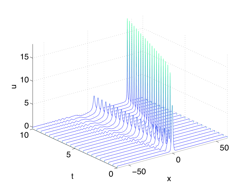
Figure 4: Solution to the BO equation for the initial data $\mathfrak{u}_{0}=10\text{sech}^{2}x$ in dependence of $t$.

The ILW equation

The formal IST theory has been given in KAS ; KSA . The direct scattering problem is associated with a Riemann-Hilbert problem in a strip of the complex plane. As the BO equation, the ILW equation possesses an infinite sequence of conserved quantities (see eg LR ) which leads to a ILW hierarchy. They can be used to provide the global well-posedness of the Cauchy problem in $H^{s}(\mathbb{R}),s>3/2$, (ABFS ).

Moreover, the fact that for large $|\xi|$, $|\xi|\text{coth}\;\xi=|\xi|(1+O(e^{-|\xi|}))$ implies that the well-posedness results are similar to those obtained for the BO equation, for instance in the energy space $H^{1/2}(\mathbb{R}).$

On the other hand, we do not know of rigorous results for the Cauchy problem using the IST method. It is likely that they would require a smallness condition on the initial data.

Explicit N-soliton solutions are given in Mat ; JE . Contrary to those of the Benjamin-Ono equation, they decay exponentially at infinity (the ILW symbol is smooth). For instance, when the ILW equation is written in the form

$$u_{t}+2uu_{x}+\frac{1}{\delta}u_{x}-L_{\delta}u_{x}=0,$$ (17)

where

$$\widehat{L_{\delta}u}(\xi)=(\xi\text{coth}\;\xi\delta)\hat{u}(\xi),$$

the 1-soliton reads (see AlTo ; J ; JE

$$u(x,t)=Q_{c,\delta}(x-ct),\quad Q_{c,\delta}(x)=\frac{a\sin a\delta}{\text{cosh}\;ax+\cos a\delta},\quad x\in\mathbb{R}$$

for arbitrary $c>0$ and $\delta>0,$ and $a$ is the unique positive solution of the transcendental equation

$$a\delta\;\text{coth}\;a\delta=(1-c\delta),\quad a\in(0,\pi/\delta).$$

Its uniqueness (up to translations) is proven in AlTo . The orbital stability of this soliton is proven in AB1 ; ABH (see also BoSo ; BSS ). We do not know of asymptotic stability results for the 1 or N-soliton similar to the corresponding ones for the BO equation. Those results should be in some sense easier than the corresponding ones for BO since the exponential decay of the solitons should make the spectral analysis of the linearized operators easier.

We show the decomposition of localized initial data into solitons and radiation in Fig. 5 and Fig. 6. Note that this case is numerically easier to treat with Fourier methods since the soliton solutions are more rapidly decreasing (exponentially instead of algebraically) than for the fKdV, fBBM and BO equations before. The different shape of the solitons is also noticeable in comparison to Fig. 4.

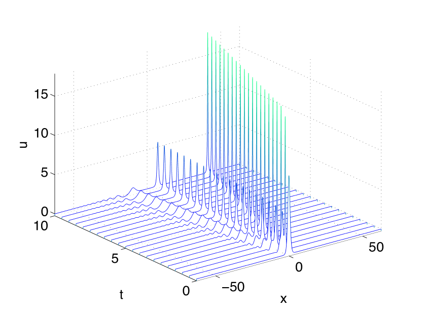
Figure 5: Solution to the ILW equation with $\delta=1$ for the initial data $\mathfrak{u}_{0}=10\text{sech}^{2}x$ in dependence of $t$.

One also sees the change in the number of emerging solitons according to the size of the initial data. As in the case of BO, fKdV, fBBM equations, predicting the number of solitary waves which seem to form from a given (smooth and localized) initial data is a challenging open question. Except for the KdV case where the solitons are related to the discrete spectrum of the associated Schrödinger equation, there does not appear to be a clear characterization of the solitons emerging from given initial data for $t\to\infty$ even for integrable equations.

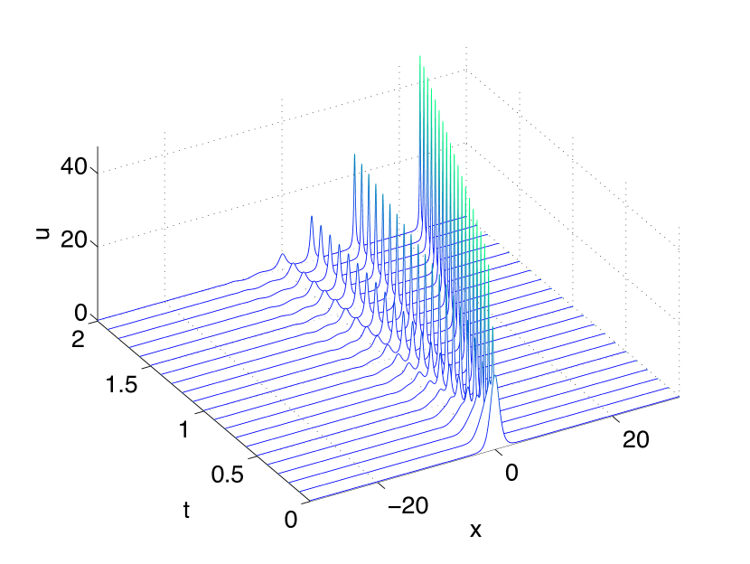
Figure 6: Solution to the ILW equation with $\delta=1$ for the initial data $\mathfrak{u}_{0}=20\text{sech}^{2}x$ in dependence of $t$.

3.3 The Gross-Pitaevskii equation

The Gross-Pitaevskii equation (GP) is a version of a nonlinear Schrödinger equation (NLS), namely

$$i\partial_{t}\Psi=\Delta\Psi+\Psi(1-|\Psi|^{2})\quad\text{on}\quad\mathbb{R}^{d}\times\mathbb{R},(d=1,2,3).$$ (18)

It is a relevant model in nonlinear optics ("dark" and "black" solitons, optical vortices), fluid mechanics (superfluidity of Helium II), Bose-Einstein condensation of ultra cold atomic gases.

At least on a formal level, the Gross-Pitaevskii equation is hamiltonian. The conserved Hamiltonian is a Ginzburg-Landau energy, namely

$$E(\Psi)=\frac{1}{2}\int_{\mathbb{R}^{d}}|\nabla\Psi|^{2}+\frac{1}{4}\int_{\mathbb{R}^{d}}(1-|\Psi|^{2})^{2}\equiv\int_{\mathbb{R}^{d}}e(\Psi),$$ (19)

associated to the natural energy space

$$\mathcal{E}(\mathbb{R}^{d})=\{v\in H^{1}_{\text{loc}}(\mathbb{R}^{d}),E(v)<+\infty\},$$

In order for $E(\Psi)$ to be finite, $|\Psi|$ should in some sense tend to 1 at infinity. Actually this "non trivial" boundary condition provides (GP) with a richer dynamics than in the case of null condition at infinity which, for a defocusing NLS type equation, is essentially governed by dispersion and scattering.

For instance, in nonlinear optics, the "dark solitons" are localized nonlinear waves (or "holes") which exist on a stable continuous wave background. The boundary condition $|\Psi(x,\cdot)|\to 1$ is due to this non-zero background.

Similarly to the energy, the momentum $\vec{P}(\Psi)=\frac{1}{2}\int_{\mathbb{R}^{N}}\langle i\nabla\Psi\ ,\Psi\rangle,$ is formally conserved.

We will denote by $p=Im\int_{\mathbb{R}^{N}}i\Psi\bar{\Psi}_{x}$, the first component of $\vec{P}$, which is hence a scalar.

Justifying the momentum (and its conservation) is one of the difficulties one has to face when dealing with the (GP) equation.

We will restrict here to the one-dimensional case, $d=1$ since the GP equation is then completely integrable ZS . We just consider

$$i\partial_{t}u+\partial^{2}_{x}u+(1-|u|^{2})u=0$$ (20)

In fact Zakharov-Shabat (1973) consider the case when $|u(x,t)|^{2}\rightarrow c>0$, $|x|\rightarrow\infty$ (propagation of waves through a condensate of constant density).

More precisely, the GP has a Lax pair $(B_{u},L_{u})$, where (for $c=1$)

$$L_{u}=i\left(\begin{array}[]{cc}1+\sqrt{3}&0\\ 0&1-\sqrt{3}\\ \end{array}\right)\partial_{x}+\left(\begin{array}[]{cc}0&\bar{u}\\ u&0\\ \end{array}\right)$$ (21)

$$B_{u}=-\sqrt{3}\left(\begin{array}[]{cc}1&0\\ 0&1\\ \end{array}\right)\partial^{2}_{x}+\left(\begin{array}[]{cc}\frac{|u|^{2}-1}{\sqrt{3}+1}&i\partial_{x}\bar{u}\\ -i\partial_{x}\bar{u}&\frac{|u|^{2}-1}{\sqrt{3}-1}\\ \end{array}\right)$$ (22)

So that u satisfies (GP) if and only if

$$\frac{d}{dt}L_{u}=[L_{u},B_{u}]$$ (23)

As a consequence, the 1 D Gross-Pitaevskii equation has an infinite number of (formally) conserved energies $E_{k},k\in\mathbb{N}$ and momentum $P_{k},k\in\mathbb{N}.$

For instance,

$$I_{5}=\int_{\mathbb{R}}\{2|u|^{6}+6|u|^{2}|u_{x}|^{2}+(\frac{d}{dx}|u|^{2})^{2}+|u_{xx}|^{2}-2\}.$$

It is of course necessary to prove rigorously that the $E_{k}$ and the $P_{k}$ are well defined and conserved by the GP flow, in a suitable functional setting.

We do not know of a complete resolution of the Cauchy problem by IST methods, including a possible decomposition into solitons. We will see however that one can get a proof of stability of the solitons by using IST techniques.

One can prove that the energy space in one dimension is identical to the Zhidkov space (see Z )

$$X^{1}(\mathbb{R})=\{u\in H^{1}_{loc}(\mathbb{R}),u_{x}\in L^{\infty}(\mathbb{R}),(1-|u|^{2})\in L^{2}(\mathbb{R})\}$$

and actually Zhidkov Z proved that the Cauchy problem for (20) is globally well-posed in $X^{1}(\mathbb{R})$ .

The one-dimensional GP equation possesses two types of solitary waves of velocity $c$, $0\leq c<\sqrt{2}$ :

• The "dark" solitons : $\mathfrak{v}_{c}(x)\equiv\sqrt{\frac{2-c^{2}}{2}}{\rm th}\Big{(}\frac{\sqrt{2-c^{2}}}{2}x\Big{)}-i\frac{c}{\sqrt{2}}$.

• The "black" soliton :

  $$\mathfrak{v}_{0}(x)={\rm th}\Big{(}\frac{x}{\sqrt{2}}\Big{)}.$$

Note that when $0<c<\sqrt{2},\>\mathfrak{v}_{c}(x)\not=0,\forall x$ while the black soliton vanishes at $x=0$.

The orbital stability of the dark soliton has been proven in BGS3 (see also Lin for the cubic-quintic case).

This case is easier since the dark soliton does not vanish and the momentum can be defined in a straightforward way. The orbital stability of the black soliton is more delicate since it vanishes at $0.$ Both PDE and IST techniques provide the result, in a slightly different form though, and this is a good opportunity to compare them.

The first method is used in BGSS3 . This is the "Hamiltonian" method (see B ; Jerry for the stability of the KdV solitary wave or CZ for the stability of the focusing NLS ground states), that is one considers the black soliton as a minimizer of the energy with fixed momentum. As previously noticed, serious difficulties arise here from the momentum (definition, conservation by the flow,…) because the black soliton vanishes at $0$.

Given any $A>0$, we consider on the energy space $X^{1}(\mathbb{R})=X^{1}$ the distance $d_{A,X^{1}}$ defined by

$$d_{A,X^{1}}(v_{1},v_{2})\equiv\|v_{1}-v_{2}\|_{L^{\infty}([-A,A])}+\|v_{1}^{\prime}-v_{2}^{\prime}\|_{L^{2}(\mathbb{R})}+\||v_{1}|-|v_{2}|\|_{L^{2}(\mathbb{R})}.$$

One can show that for $v\in X^{1},$ $|v(x)|\rightarrow 1$ as $|x|\rightarrow\infty,$ (but not $v$ itself).

We have the orbital stability result (BGSS3 ):

Theorem 3.1

Assume that $v_{0}\in X^{1}$ and consider the global in time solution $v$ to (GP) with initial datum $v_{0}$. Given any numbers $\varepsilon>0$ and $A>0$, there exists some positive number $\delta$, such that if

$$d_{A,X^{1}}(v_{0},\mathfrak{v}_{0})\leq\delta,$$ (24)

then, for any $t\in\mathbb{R}$, there exist numbers $a(t)$ and $\theta(t)$ such that

$$d_{A,X^{1}}\big{(}v(\cdot+a(t),t),\exp(i\theta(t))\ \mathfrak{v}_{0}(\cdot)\big{)}<\varepsilon.$$ (25)

We also have a control of the shift $a(t)$:

Theorem 3.2

Given any numbers $\varepsilon>0$, sufficiently small, and $A>0$, there exists some constant $K$, only depending on $A$, and some positive number $\delta>0$ such that, if $v_{0}$ and $v$ are as in the previous Theorem, then

$$|a(t)|\leq K\varepsilon(1+|t|),$$ (26)

for any $t\in\mathbb{R}$, and for any of the points $a(t)$ as above.

We will not give a proof of the previous results (see BGSS3 ) but just explain how to extend the definition of the momentum $P(v)=\frac{1}{2}\int_{\mathbb{R}}\langle iv,v^{\prime}\rangle$ for general functions in $X^{1}.$

• Assume $v\in X^{1}$ and $v=\exp(i\phi).$

Then $\langle iv,v^{\prime}\rangle=\phi^{\prime}\in L^{2}(\mathbb{R})$ and $P(v)\equiv\frac{1}{2}[\phi(+\infty)-\phi(-\infty)].$

This is meaningful if

$$v\in Z^{1}=\Big{\{}v\in X^{1},\ {\rm s.t.}\ v_{\pm\infty}=\lim_{x\to\pm\infty}v(x)\ {\rm exist}\Big{\}},$$

but not for any arbitrary phase $\phi$ whose gradient is in $L^{2}$.

Let

$$\tilde{X^{1}}=\{v\in X^{1},\ {\rm s.t.}\ |v(x)|>0,\ \forall x\in\mathbb{R}\}.$$

For $v\in\tilde{X^{1}}$, $v=\rho\exp(i\phi)$, so that $\langle iv,v^{\prime}\rangle=\rho^{2}\phi^{\prime}$. If $v\in\tilde{Z^{1}}\equiv\tilde{X^{1}}\cap Z^{1}$, one has

$$P(v)=\frac{1}{2}\int_{\mathbb{R}}\rho^{2}\phi^{\prime}=\frac{1}{2}\int_{\mathbb{R}}(\rho^{2}-1)\phi^{\prime}+\frac{1}{2}\int_{\mathbb{R}}\phi^{\prime}=\frac{1}{2}\int_{\mathbb{R}}(\rho^{2}-1)\phi^{\prime}+\frac{1}{2}\big{[}\phi\big{]}_{-\infty}^{+\infty}.$$ (27)

This is well controlled since by Cauchy-Schwarz

$$|\int_{\mathbb{R}}(\rho^{2}-1)\phi^{\prime}|\leq\frac{2}{\delta^{2}}E(v)$$

where

$$\delta=inf\{|v(x)|,x\in\mathbb{R}\}.$$

• The momentum for maps with zeroes:

Lemma 1

Let $v\in Z^{1}$. Then, the limit

$$\mathcal{P}(v)=\underset{R\to+\infty}{\lim}P_{R}(v)\equiv\lim_{R\to+\infty}\int_{-R}^{R}\langle iv,v^{\prime}\rangle$$

exists. Moreover, if $v$ belongs to $\tilde{Z^{1}}$, then

$$\mathcal{P}(v)=\frac{1}{2}\int_{\mathbb{R}}(\rho^{2}-1)\phi^{\prime}+\frac{1}{2}\big{[}\phi\big{]}_{-\infty}^{+\infty}.$$

• Example the black soliton $\mathfrak{v}_{0}$: since $\mathfrak{v}_{0}$ is real-valued, $\langle i\mathfrak{v}_{0},\mathfrak{v}_{0}^{\prime}\rangle=0$ and $\mathcal{P}(\mathfrak{v}_{0})=0.$

• Elementary observation. Let $V_{0}\in Z^{1}$ and $w\in H^{1}(\mathbb{R}).$ Then, $V_{0}+w\in Z^{1}$ and

  $$\mathcal{P}(V_{0}+w)=\mathcal{P}(V_{0})+\frac{1}{2}\int_{\mathbb{R}}\langle iw,w^{\prime}\rangle+\int_{\mathbb{R}}\langle iw,V_{0}^{\prime}\rangle.$$

• Note that besides $\mathcal{P}(V_{0})$ the integrals are definite ones.

• The renormalized and the untwisted momentum.

The renormalized momentum $p$ is defined for $v\in\tilde{X_{1}}$ by

$$p(v)=\frac{1}{2}\int_{\mathbb{R}}(\varrho^{2}-1)\varphi^{\prime},$$ (28)

as seen before, if $v$ belongs to $\tilde{Z^{1}}$, then,

$$p(v)=\mathcal{P}(v)-\frac{1}{2}\big{[}\varphi\big{]}_{-\infty}^{+\infty}.$$

If $v\in Z^{1}\setminus\tilde{Z^{1}}$, the integral is a priori not well-defined since the phase $\varphi$ is not globally defined. Nevertheless, the argument $\arg{v}$ of $v$ is well-defined at infinity as an element of $\mathbb{R}/2\pi\mathbb{Z}$. For $v\in Z^{1}$, one introduces the untwisted momentum

$$[p](v)=\Big{(}\mathcal{P}(v)-\frac{1}{2}\big{(}\arg{v(+\infty)}-\arg{v(-\infty)}\big{)}\Big{)}\ {\rm mod}\ \pi,$$

which is hence an element of $\mathbb{R}/\pi\mathbb{Z}$. A remarkable fact concerning $[p]$ is that its definition extends to the whole space $X^{1}$, although for arbitrary maps in $X^{1}$, the quantity $\arg{v(+\infty)}-\arg{v(-\infty)}$ may not exist.

Lemma 2

Assume that $v$ belongs to $X^{1}$. Then the limit

$$[p](v)=\lim_{R\to+\infty}\bigg{(}\int_{-R}^{R}\langle iv,v^{\prime}\rangle-\frac{1}{2}\big{(}\arg{v(R)}-\arg{v(-R)}\big{)}\bigg{)}\ {\rm mod}\ \pi$$

exists. Moreover, if $v$ belongs to $\tilde{X^{1}}$, then

$$[p](v)=p(v)\ {\rm mod}\ \pi.$$ (29)

One has also:

• Let $V_{0}\in X^{1}$ and $w\in H^{1}(\mathbb{R})$. Then, $V_{0}+w\in X^{1}$ and

  $$[p](V_{0}+w)=[p](V_{0})+\frac{1}{2}\int_{\mathbb{R}}\langle iw,w^{\prime}\rangle+\int_{\mathbb{R}}\langle iw,V_{0}^{\prime}\rangle\ {\rm mod}\ \pi.$$ (30)

• The evolution preserves the untwisted momentum:

Lemma 3

Assume $v_{0}\in X^{1}$, and let $v$ be the solution to (GP) with initial datum $v_{0}$. Then,

$$[p](v(\cdot,t))=[p](v_{0}),\ \forall t\in\mathbb{R}.$$

If moreover $v_{0}\in Z^{1}$, then $v(t)$ belongs to $Z^{1}$ for any $t\in\mathbb{R}$, and

$$\mathcal{P}(v(\cdot,t))=\mathcal{P}(v_{0}),\ \forall t\in\mathbb{R}.$$

The orbital stability of the dark soliton ($0<c<\sqrt{2})$ is based on the minimization problem:

$$E_{\min}(\mathfrak{p})=\inf\{E(v),v\in\tilde{X^{1}}\;\text{s.t.}\;p(v)=\mathfrak{p}\}.$$

For map having zeroes like $\mathfrak{v}_{0}$, one should use the untwisted momentum and consider instead

$$\mathfrak{E}_{\min}\Big{(}\frac{\pi}{2}\Big{)}\equiv\inf\big{\{}E(v),v\in X^{1}\ \text{s.t.}\;[p](v)=\frac{\pi}{2}\;\text{ mod}\;\pi\big{\}}.$$ (31)

We now turn to the second approach using IST in GZ which avoids the renormalization by factors of modulus 1 in Theorem 3.1, at least for sufficiently smooth and decaying perturbations.

Theorem 3.3

Assume that the initial datum of (1.1) has the form: $u_{0}(x)=U_{0}(x)+\epsilon u_{1}(x),U_{0}(x)=\text{tanh}\left(\frac{x}{\sqrt{2}}\right),$ where $u_{1}(x)$ satisfies the following condition,

$$\sup_{x\in\mathbb{R}}|(1+x^{2})^{2}\partial^{k}u_{1}(x)|\leq 1,\quad\text{for}\;k\leq 3.$$

$$\forall t\in\mathbb{R},\quad\exists\;y(t)\in\mathbb{R},\quad|\tau_{y(t)}u(.,t)-U_{0}|_{\infty}\leq C\epsilon,\quad\text{for}\;0\leq t<+\infty.$$

Using a classical functional analytic argument, Theorem 3.3 easily yields the orbital stability, at least for sufficiently smooth and decaying perturbations GZ :

Corollary 1

For every $\delta>0$ there exists $\epsilon>0$ such that, if

$$\sup_{x\in\mathbb{R}}|(1+x^{2})^{2}\partial^{k}u_{1}(x)|\leq 1,\quad\text{for}\;k\leq 3,$$

then the solution $u$ of (20) satisfies:

$$\forall t\in\mathbb{R},\;\exists y(t)\in\mathbb{R},\quad d_{E}(\tau_{y(t)}u(t),U_{0})\leq\delta.$$

Remark 6

As previously noticed Theorem 3.3 improves on Theorem 3.1, 3.2 since it does not require a rotation factor. On the other hand it deals with a narrower class of perturbations and does not provide an evaluation of the time shift.

One can combine PDE and IST techniques as for instance in the long wave limit of the GP equation which we describe now.

The transonic (long wave, small amplitude) limit of KGP to KP I in 2D or KdV in 1D is quite a generic phenomenon for nonlinear dispersive systems. A good example is that of the water wave systems (incompressible Euler with upper free surface).

While the consistency of the approximation is relatively easy to obtain, the stability (and thus the convergence) of the approximation is much more delicate, specially if one looks for the optimal error estimates on the correct time scales.

Kuznetsov and Zakharov ZK have observed formally that the KdV equation provides a good approximation of long-wave small amplitude solutions to the 1D Gross-Pitaevskii equation. We recall here briefly a rigorous proof of this fact BGSS1 (see also CR for a different approach which dose not provide an error estimate and BGSS2 for a similar analysis for two-way propagation leading to a coupled system of KdV equations). We thus start from the 1D GP equation

$$i\partial_{t}\Psi+\partial_{x}^{2}\Psi=\Psi(|\Psi|^{2}-1)\quad\text{on}\quad\mathbb{R}\times\mathbb{R},\quad\Psi(.,0)=\Psi_{0},$$ (32)

$$|\Psi(x,t)|\to 1,\text{as}\quad|x|\to+\infty,$$ (33)

and recall the formal conserved quantities

$$E(\Psi)=\frac{1}{2}\int_{\mathbb{R}}|\partial_{x}\Psi|^{2}+\frac{1}{4}\int_{\mathbb{R}}(1-|\Psi|^{2})^{2}\equiv\int_{\mathbb{R}}e(\Psi).$$

$$P(\Psi)=\frac{1}{2}\int_{\mathbb{R}}\langle i\partial_{x}\Psi,\Psi\rangle.$$

One can prove (see for instance Ga2 ) well-posedness in Zhidkov spaces :

$$X^{k}(\mathbb{R})=\{u\in L^{1}_{\rm loc}(\mathbb{R},\mathbb{C}),\ {\rm s.t.}\ E(u)<+\infty,\ {\rm and}\ \partial_{x}u\in H^{k-1}(\mathbb{R})\},$$

Theorem 3.4

Let $k\in\mathbb{N}^{*}$ and $\Psi_{0}\in X^{k}(\mathbb{R})$. Then, there exists a unique solution $\Psi(\cdot,t)$ in $\mathcal{C}^{0}(\mathbb{R},X^{k}(\mathbb{R}))$ to (32) with initial data $\Psi_{0}$. If $\Psi_{0}$ belongs to $X^{k+2}(\mathbb{R})$, then the map $t\mapsto\Psi(\cdot,t)$ belongs to $\mathcal{C}^{1}(\mathbb{R},X^{k}(\mathbb{R}))$ and $\mathcal{C}^{0}(\mathbb{R},X^{k+2}(\mathbb{R}))$. Moreover, the flow map $\Psi_{0}\mapsto\Psi(\cdot,T)$ is continuous on $X^{k}(\mathbb{R})$ for any fixed $T\in\mathbb{R}$.

Remark 7

One can prove conservation of energy and momentum (under suitable assumptions).

We recall that if $\Psi$ does not vanish, one may write (Madelung transform)

$$\Psi=\sqrt{\rho}\exp i\varphi.$$

This leads to the hydrodynamic form of the equation, with $v=2\partial_{x}\varphi,$

$$\left\{\begin{array}[]{ll}\partial_{t}\rho+\partial_{x}(\rho v)=0,\\ \rho(\partial_{t}v+v.\partial_{x}v)+\partial_{x}(\rho^{2})=\rho\partial_{x}\Big{(}\frac{\partial_{x}^{2}\rho}{\rho}-\frac{|\partial_{x}\rho|^{2}}{2\rho^{2}}\Big{)},\end{array}\right.$$ (34)

which can be seen as a compressible Euler system with pressure law $p(\rho)=\rho^{2}$ and a quantum pressure term.

It is shown in BDS that (32) or (34) can be approximated by the linear wave equation. We justify here the long wave approximation on larger time scales $\mathcal{O}(\varepsilon^{-3})$ and, following Kuznetsov and Zakharov, introduce the slow variables :

$$X=\varepsilon(x+\sqrt{2}t),\ {\rm and}\ \tau=\frac{\varepsilon^{3}}{2\sqrt{2}}t.$$ (35)

This corresponds to a reference frame traveling to the left with velocity $\sqrt{2}$ in the original variables $(x,t)$. In this frame the left going wave is stationary while the right going wave has a speed $8\varepsilon^{-2}$ and is appropriate to study waves traveling to the left (we need to impose additional assumptions which imply the smallness of the right going waves).

We define the rescaled functions $N_{\varepsilon}$ and $\Theta_{\varepsilon}$ as follows

$$\begin{split}N_{\varepsilon}(X,\tau)&=\frac{6}{\varepsilon^{2}}\eta(x,t)=\frac{6}{\varepsilon^{2}}\eta\Big{(}\frac{X}{\varepsilon}-\frac{4\tau}{\varepsilon^{3}},\frac{2\sqrt{2}\tau}{\varepsilon^{3}}\Big{)},\\ \Theta_{\varepsilon}(X,\tau)&=\frac{6\sqrt{2}}{\varepsilon}\varphi(x,t)=\frac{6\sqrt{2}}{\varepsilon}\varphi\Big{(}\frac{X}{\varepsilon}-\frac{4\tau}{\varepsilon^{3}},\frac{2\sqrt{2}\tau}{\varepsilon^{3}}\Big{)},\end{split}$$ (36)

where $\Psi=\varrho\exp(i\varphi)$ and $\eta=1-\varrho^{2}=1-|\Psi|^{2}$.

Theorem 3.5

BGSS1 Let $\varepsilon>0$ be given and assume that the initial data $\Psi_{0}(\cdot)=\Psi(\cdot,0)$ belong to $X^{4}(\mathbb{R})$ and satisfy the assumption

$$\|N_{\varepsilon}^{0}\|_{H^{3}(\mathbb{R})}+\varepsilon\|\partial^{4}_{x}N_{\varepsilon}^{0}\|_{L^{2}(\mathbb{R})}+\|\partial_{x}\Theta_{\varepsilon}^{0}\|_{H^{3}(\mathbb{R})}\leq K_{0}.$$ (37)

Let $\mathcal{N}_{\varepsilon}$ and $\mathcal{M}_{\varepsilon}$ denote the solutions to the Korteweg-de Vries equation

$$\partial_{\tau}N+\partial_{x}^{3}N+N\partial_{x}N=0$$ (38)

with initial data $N_{\varepsilon}^{0}$, respectively $\partial_{x}\Theta_{\varepsilon}^{0}$. There exist positive constants $\varepsilon_{0}$ and $K_{1}$, depending possibly only on $K_{0}$ such that, if $\varepsilon\leq\varepsilon_{0}$, we have for any $\tau\in\mathbb{R}$,

$$\begin{split}\|\mathcal{N}_{\varepsilon}&(\cdot,\tau)-N_{\varepsilon}(\cdot,\tau)\|_{L^{2}(\mathbb{R})}+\|\mathcal{M}_{\varepsilon}(\cdot,\tau)-\partial_{x}\Theta_{\varepsilon}(\cdot,\tau)\|_{L^{2}(\mathbb{R})}\\ &\leq K_{1}\big{(}\varepsilon+\|N_{\varepsilon}^{0}-\partial_{x}\Theta_{\varepsilon}^{0}\|_{H^{3}(\mathbb{R})}\big{)}\exp(K_{1}|\tau|).\end{split}$$ (19)

• This is a convergence result to the KdV equation for appropriate prepared initial data.

• Since the norms involved are translation invariant, the KdV approximation can be only valid if the right going waves are negligible. This is the role of the term $\|N_{\varepsilon}^{0}-\partial_{x}\Theta_{\varepsilon}^{0}\|_{H^{3}(\mathbb{R})}.$

• In particular, if $\|N_{\varepsilon}^{0}-\partial_{x}\Theta_{\varepsilon}^{0}\|_{H^{3}(\mathbb{R})}\leq C\varepsilon^{\alpha}$, with $\alpha>0$, then the approximation is valid on a time interval $t\in[0,S_{\varepsilon}]$ with $S_{\varepsilon}=o(\varepsilon^{-3}|\log(\varepsilon)|)$. Moreover, if $\|N_{\varepsilon}^{0}-\partial_{x}\Theta_{\varepsilon}^{0}\|_{H^{3}(\mathbb{R})}$ is of order $\mathcal{O}(\varepsilon)$, then the approximation error remains of order $\mathcal{O}(\varepsilon)$ on a time interval $t\in[0,S_{\varepsilon}]$ with $S_{\varepsilon}=\mathcal{O}(\varepsilon^{-3})$.

The functions $N_{\varepsilon}$ and $\partial_{X}\Theta_{\varepsilon}$ are rigidly constrained one to the other:

Theorem 3.6

Let $\Psi$ be a solution to GP in $\mathcal{C}^{0}(\mathbb{R},H^{4}(\mathbb{R}))$ with initial data $\Psi^{0}$. Assume that (37) holds. Then, there exists some positive constant $K$, which does not depend on $\varepsilon$ nor $\tau$, such that

$$\|N_{\varepsilon}(\cdot,\tau)\pm\partial_{X}\Theta_{\varepsilon}(\cdot,\tau)\|_{L^{2}(\mathbb{R})}\leq\|N_{\varepsilon}^{0}\pm\partial_{X}\Theta_{\varepsilon}^{0}\|_{L^{2}(\mathbb{R})}+K\varepsilon^{2}\big{(}1+|\tau|\big{)},*$$ (20)

for any $\tau\in\mathbb{R}$.

The approximation errors provided by the previous theorems diverge as time increases. Concerning the weaker notion of consistency, we have the following result whose peculiarity is that the bounds are independent of time.

Theorem 3.7

Let $\Psi$ be a solution to GP in $\mathcal{C}^{0}(\mathbb{R},H^{4}(\mathbb{R}))$ with initial data $\Psi^{0}$. Assume that (37) holds. Then, there exists some positive constant $K$, which does not depend on $\varepsilon$ nor $\tau$, such that

$$\|\partial_{\tau}U_{\varepsilon}+\partial^{3}_{X}U_{\varepsilon}+U_{\varepsilon}\partial_{X}U_{\varepsilon}\|_{L^{2}(\mathbb{R})}\leq K(\varepsilon+\|N_{\varepsilon}^{0}-\partial_{X}\Theta_{\varepsilon}\|_{H^{3}(\mathbb{R})}),$$ (21)

for any $\tau\in\mathbb{R}$, where $U_{\varepsilon}=\frac{N_{\varepsilon}+\partial_{x}\Theta_{\varepsilon}}{2}$.

• One gets explicit bounds for the traveling wave solutions

$\Psi(x,t)=v_{c}(x+ct)$. Solutions do exist for any value of the speed $c$ in the interval $[0,\sqrt{2})$. Next, we choose the wave-length parameter to be $\varepsilon=\sqrt{2-c^{2}}$, and take as initial data $\Psi_{\varepsilon}$ the corresponding wave $v_{c}$. We consider the rescaled function

$$\nu_{\varepsilon}(X)=\frac{6}{\varepsilon^{2}}\eta_{c}\Big{(}\frac{x}{\varepsilon}\Big{)},$$

where $\eta_{c}\equiv 1-|v_{c}|^{2}$. The explicit integration of the travelling wave equation for $v_{c}$ leads to the formula

$$\nu_{\varepsilon}(X)=\nu(x)\equiv\frac{3}{{\rm ch}^{2}\big{(}\frac{X}{2}\big{)}}.$$

The function $\nu$ is the classical soliton to the Korteweg-de Vries equation, which is moved by the KdV flow with constant speed equal to $1$, so that

$$\mathcal{N}_{\varepsilon}(X,\tau)=\nu(X-\tau).$$

On the other hand, we deduce from (36) that $N^{0}_{\varepsilon}=\nu$, so that

$$N_{\varepsilon}(X,\tau)=\nu\Big{(}X-\frac{4}{\varepsilon^{2}}\Big{(}1-\sqrt{1-\frac{\varepsilon^{2}}{2}}\Big{)}\tau\Big{)}.$$

Therefore, we have for any $\tau\in\mathbb{R}$,

$$\|\mathcal{N}_{\varepsilon}(\cdot,\tau)-N_{\varepsilon}(\cdot,\tau)\|_{L^{2}(\mathbb{R})}=\mathcal{O}(\varepsilon^{2}\tau).$$

This suggests that the $\varepsilon$ error in the main theorem should be of order $\varepsilon^{2}$. This is proved in BGSS2 at a cost of higher regularity on the initial data (and also for a two way propagation, described by a system of two KdV equations).

We now give some elements of the proofs which rely on energy methods.

We first write the equations for $N_{\varepsilon}$ and $\Theta_{\varepsilon}$:

$$\partial_{X}N_{\varepsilon}-\partial_{x}^{2}\Theta_{\varepsilon}+\frac{\varepsilon^{2}}{2}\Big{(}\frac{1}{2}\partial_{\tau}N_{\varepsilon}+\frac{1}{3}N_{\varepsilon}\partial_{X}^{2}\Theta_{\varepsilon}+\frac{1}{3}\partial_{X}N_{\varepsilon}\partial_{X}\Theta_{\varepsilon}\Big{)}=0,$$ (22)

and

$$\partial_{X}\Theta_{\varepsilon}-N_{\varepsilon}+\frac{\varepsilon^{2}}{2}\Big{(}\frac{1}{2}\partial_{\tau}\Theta_{\varepsilon}+\frac{\partial_{X}^{2}N_{\varepsilon}}{1-\frac{\varepsilon^{2}}{6}N_{\varepsilon}}+\frac{1}{6}(\partial_{X}\Theta_{\varepsilon})^{2}\Big{)}+\frac{\varepsilon^{4}}{24}\frac{(\partial_{X}N_{\varepsilon})^{2}}{(1-\frac{\varepsilon^{2}}{6}N_{\varepsilon})^{2}}=0.$$ (23)

The leading order in this expansion is provided by $N_{\varepsilon}-\partial_{X}\Theta_{\varepsilon}$ and its spatial derivative, so that an important step is to keep control on this term. In view of (22) and (23) and d’Alembert decomposition, we are led to introduce the new variables $U_{\varepsilon}$ and $V_{\varepsilon}$ defined by

$$U_{\varepsilon}=\frac{N_{\varepsilon}+\partial_{X}\Theta_{\varepsilon}}{2},\ {\rm and}\ V_{\varepsilon}=\frac{N_{\varepsilon}-\partial_{X}\Theta_{\varepsilon}}{2},$$

and compute the relevant equations for $U_{\varepsilon}$ and $V_{\varepsilon}$,

$$\partial_{\tau}U_{\varepsilon}+\partial_{X}^{3}U_{\varepsilon}+U_{\varepsilon}\partial_{X}U_{\varepsilon}=-\partial_{X}^{3}V_{\varepsilon}+\frac{1}{3}\partial_{X}\big{(}U_{\varepsilon}V_{\varepsilon}\big{)}+\frac{1}{6}\partial_{X}\big{(}V_{\varepsilon}^{2}\big{)}-\varepsilon^{2}R_{\varepsilon},$$ (24)

and

$$\partial_{\tau}V_{\varepsilon}+\frac{8}{\varepsilon^{2}}\partial_{x}V_{\varepsilon}=\partial_{X}^{3}U_{\varepsilon}+\partial_{X}^{3}V_{\varepsilon}+\frac{1}{2}\partial_{x}(V_{\varepsilon}^{2})-\frac{1}{6}\partial_{x}(U_{\varepsilon})^{2}-\frac{1}{3}\partial_{X}(U_{\varepsilon}V_{\varepsilon})+\varepsilon^{2}R_{\varepsilon},$$ (25)

where the remainder term $R_{\varepsilon}$ is given by the formulae

$$R_{\varepsilon}=\frac{N_{\varepsilon}\partial_{X}^{3}N_{\varepsilon}}{6(1-\frac{\varepsilon^{2}}{6}N_{\varepsilon})}+\frac{(\partial_{X}N_{\varepsilon})(\partial_{X}^{2}N_{\varepsilon})}{3(1-\frac{\varepsilon^{2}}{6}N_{\varepsilon})^{2}}+\frac{\varepsilon^{2}}{36}\frac{(\partial_{X}N_{\varepsilon})^{3}}{(1-\frac{\varepsilon^{2}}{6}N_{\varepsilon})^{3}}.$$ (26)

The main step is to show that the RHS of the equation for $U_{\varepsilon}$ is small in suitable norms. In particular one must show that $V_{\varepsilon}$ which is assumed to be small at time $\tau=0$ remains small, and that $U_{\varepsilon}$, assumed to be bounded at time $\tau=0$, remains bounded in appropriate norms. We use in particular various conservation laws provided by the integrability of the one-dimensional Gross-Pitaevskii equation.

• For instance we use the conservation of momentum and energy to get the $L^{2}$ estimates.

• It turns out that the other conservation laws behave as higher order energies and higher order momenta. We use them to get :

Theorem 3.8

Let $\Psi$ be a solution to (GP) in $\mathcal{C}^{0}(\mathbb{R},H^{4}(\mathbb{R}))$ with initial data $\Psi^{0}$. Assume that (37) holds. Then, there exists some positive constant $K$, which does not depend on $\varepsilon$ nor $\tau$, such that

$$\|N_{\varepsilon}(\cdot,\tau)\|_{H^{3}(\mathbb{R})}+\varepsilon\|\partial_{X}^{4}N_{\varepsilon}(\cdot,\tau)\|_{L^{2}(\mathbb{R})}+\|\partial_{X}\Theta_{\varepsilon}(\cdot,\tau)\|_{H^{3}(\mathbb{R})}\leq K,$$ (27)

and

$$\|N_{\varepsilon}(\cdot,\tau)\pm\partial_{X}\Theta_{\varepsilon}(\cdot,\tau)\|_{H^{3}(\mathbb{R})}\leq K\big{(}\|N_{\varepsilon}^{0}\pm\partial_{X}\Theta_{\varepsilon}^{0}\|_{H^{3}(\mathbb{R})}+\varepsilon\big{)},$$ (28)

for any $\tau\in\mathbb{R}$.

The proof of the previous result led to a number of facts linked to integrability which have independent interest:

• It provides expressions for the invariant quantities of GP and prove that they are well-defined in the spaces $X^{k}(\mathbb{R})$. Their expressions are not a straightforward consequence of the induction formula of Zakharov and Shabat since many renormalizations have to be performed to give them a sound mathematical meaning.

• It stablishes rigorously that they are conserved by the GP flow in the appropriate functional spaces.

• It displays a striking relationship between the conserved quantities of the Gross-Pitaevskii equation and the KdV invariants:

  $$\mathcal{E}_{k}(N,\partial_{X}\Theta)-\sqrt{2}\mathcal{P}_{k}(N,\partial_{x}\Theta)=E_{k}^{KdV}\Big{(}\frac{N-\partial_{X}\Theta}{2}\Big{)}+\mathcal{O}(\varepsilon^{2}).$$

It would be interesting to investigate further connections between the IST theories of the KdV and GP equations.

Remark 8

We do not know of a rigorous result by IST methods describing the qualitative behavior of a solution (solitons+radiation,…) of the GP equation corresponding to a smooth and localized initial data.

4 The Kadomtsev-Petviashvili equation

The Kadomtsev-Petviashvili equations are universal asymptotic models for dispersive systems in the weakly nonlinear, long wave regime, when the wavelengths in the transverse direction are much larger than in the direction of propagation.

The (classical) Kadomtsev-Petviashvili (KP) equations read

$$(u_{t}+u_{xxx}+uu_{x})_{x}\pm u_{yy}=0.$$ (29)

Actually the (formal) analysis) in KaPe consists in looking for a weakly transverse perturbation of the one-dimensional transport equation

$$u_{t}+u_{x}=0.$$ (30)

This perturbation amounts to adding a nonlocal term, leading to

$$u_{t}+u_{x}+\frac{1}{2}\partial_{x}^{-1}u_{yy}=0.$$ (31)

Here the operator $\partial_{x}^{-1}$ is defined via Fourier transform,

$$\widehat{\partial_{x}^{-1}f}(\xi)=\frac{i}{\xi_{1}}\widehat{f}(\xi),\,\text{where}\;\xi=(\xi_{1},\xi_{2}).$$

When this same formal procedure is applied to the KdV equation written in the context of water waves (where $T\geq 0$ is the Bond number measuring the surface tension effects)

$$u_{t}+u_{x}+uu_{x}+(1-\frac{1}{3}T)u_{xxx}=0,\;x\in\mathbb{R},\;t\geq 0,$$ (32)

this yields the KP equation in the form

$$u_{t}+u_{x}+uu_{x}+(1-\frac{1}{3}T)u_{xxx}+\frac{1}{2}\partial_{x}^{-1}u_{yy}=0.$$ (33)

By change of frame and scaling, (33) reduces to (29) with the $+$ sign (KP II) when $T<\frac{1}{3}$ and the $-$ sign (KP I) when $T>\frac{1}{3}$.

Of course the same formal procedure could be applied to any one-dimensional weakly nonlinear dispersive equation of the form

$$u_{t}+u_{x}+f(u)_{x}-Lu_{x}=0,\;x\in\mathbb{R},\;t\geq 0,$$ (34)

where $f(u)$ is a smooth real-valued function (most of the time polynomial) and $L$ a linear operator taking into account the dispersion and defined in Fourier variable by

$$\mathfrak{F}(Lu)(\xi)=p(\xi)\mathfrak{F}u(\xi),$$ (35)

where the symbol $p(\xi)$ is real-valued. The KdV equation corresponds for instance to $f(u)=\frac{1}{2}u^{2}$ and $p(\xi)=-\xi^{2}.$

This leads to a class of generalized KP equations

$$u_{t}+u_{x}+f(u)_{x}-Lu_{x}+\frac{1}{2}\partial_{x}^{-1}u_{yy}=0,\;x\in\mathbb{R},\;t\geq 0.$$ (36)

Thus one could have KP versions of the Benjamin-Ono, Intermediate Long Wave, Kawahara, etc… equations, but only the KP I and KP II equations are completely integrable (in some sense).

Let us notice, at this point, that alternative models to KdV-type equations (34) are the equations of Benjamin–Bona–Mahony (BBM) type

$$u_{t}+u_{x}+uu_{x}+Lu_{t}=0$$ (37)

with corresponding two-dimensional “KP–BBM-type models” (in the case $p(\xi)\geq 0$)

$$u_{t}+u_{x}+uu_{x}+Lu_{t}+\partial_{x}^{-1}\partial_{y}^{2}u=0$$ (38)

or, in the derivative form

$$(u_{t}+u_{x}+uu_{x}+Lu_{t})_{x}+\partial_{y}^{2}u=0$$ (39)

and free group

$$S(t)=e^{-t(I+L)^{-1}[\partial_{x}+\partial_{x}^{-1}\partial_{y}^{2}]}\,\,.$$

It was only after the seminal paper KaPe that Kadomtsev-Petviashvili type equations have been derived as asymptotic weakly nonlinear models (under an appropriate scaling) in various physical situations (see AS for a formal derivation in the context of water waves La ; La2 , LS for a rigorous one in the same context) and Ka in a different context.

Remark 9

In some physical contexts (not in water waves!) one could consider higher dimensional transverse perturbations, which amounts to replacing $\partial_{x}^{-1}u_{yy}$ in (46) by $\partial_{x}^{-1}\Delta^{\perp}u$, where $\Delta^{\perp}$ is the Laplace operator in the transverse variables.

For instance, as in the one-dimensional case the KP I equation (in both two and three dimensions) also describes after a suitable scaling the long wave transonic limit of the Gross-Pitaevskii equation (see BGS for the solitary waves and CR for the Cauchy problem).

Note again that in the classical KP equations, the distinction between KP I and KP II arises from the sign of the dispersive term in $x$.

4.1 KP by Inverse Scattering

It is usual in the Inverse Scattering community to write the Kadomstsev-Petviashvili equations as

$$\partial_{x}(\partial_{t}u+6u\partial_{x}u+\partial^{3}_{x}u)=-3\sigma^{2}\partial_{t}^{2}u,$$ (40)

where $\sigma^{2}=1$ corresponding to KP II and $\sigma^{2}=-1$ to KP I.

The KP II equation

The direct scattering problem is associated to the heat equation with the initial potential $u_{0}(x,y):$

$$-\partial_{y}\phi+\partial_{x}^{2}\phi+2ik\partial_{x}\phi+u_{0}\phi=0,\quad\phi_{|k|\to\infty}=1,$$ (41)

and the scattering data are calculated by

$$F(k)=(2\pi)^{-1}\text{sign}(\mathcal{R}e\;k)\int_{\mathbb{R}^{2}}u_{0}(x,y)\phi(x,y,k)\text{exp}\{-i(k+\bar{k})x-(k^{2}-\bar{k}^{2})y\}dxdy.$$

The time evolution of the scattering data is trivial :

$$\mathcal{F}(k,t)=F(k)\text{exp}(4it(k^{3}+\bar{k}^{3})).$$

The inverse scattering problem, that is the reconstruction of the potential $u(x,y,t)$ reduces to a $\bar{\partial}$ problem :

$$\left\{\begin{array}[]{l}\partial_{k}\phi=\psi F(-k)\text{exp}(itS),\\ \partial_{k}\psi=-\phi F(k)\text{exp}(-itS)\par\end{array}\right.$$ (42)

$\begin{pmatrix}\phi\\ \psi\end{pmatrix}$ $\to$ $\begin{pmatrix}1\\ 1\end{pmatrix}$ as $|k|\to\infty,$

and where

$$S=4(k^{3}+\bar{k}^{3})+(k+\bar{k})\xi-i(k^{2}-\bar{k}^{2})\eta,\;\xi=x/t,\;\text{and}\;\eta=y/t.$$

It turns out that the direct scattering problem can be solved only for small data in spaces of type $L^{1}\cap L^{2},$ yielding global existence of uniformly bounded (in the space of $L^{2}$ functions with bounded Fourier transform) solutions of KP II provided $u_{0}$ has small derivatives up to order $8$ in $L^{1}\cap L^{2}(\mathbb{R}^{2})$ (W ). We will see that PDE methods provide a much better result.

Remark 10

In Gr , Grinevich has proven that the direct spectral problem is nonsingular for real nonsingular exponentially decaying at infinity, arbitrary large potentials. Unfortunately, this does not mean that the solution of the direct scattering problem belongs to an appropriate functional class for existence of an inverse scattering problem when $t>0.$ In fact, the direct problem and inverse problem are different and the solvability of the first one does not give the automatic solvability of the second one.

Remark 11

Since KP II type equations do not have localized solitary waves (deBS ), one expects the large time behavior of solutions to be just governed by scattering. In particular, one can conjecture safely than the global solutions of KP II (that exist by the result of Bourgain, see Bourgain3 and the discussion below) should decay in the sup-norm as $1/t.$ This is also suggested by our numerical simulations KS2 .

A very precise asymptotics as $t\to\infty$ is given in Ki2 (see also Ki ) for a specific class of scattering data. It differs according to different domains in the $(x,y,t)$ space, expressed in terms of the variables $\xi=x/t$ and $\eta=y/t$. The main term of the asymptotics has order $O(1/t)$ (which is exactly the decay rate of the free linear evolution, see Sa ) and rapidly oscillates. In one of the domains, the decay is $o(1/t).$ It is not clear however how the hypothesis on the scattering data translate to the space of initial data.

On the other hand, the Inverse Scattering method has been used formally in AV and rigorously in AV2 to study the Cauchy problem for the KP II equation with nondecaying data along a line, that is $u(0,x,y)=u_{\infty}(x-vy)+\phi(x,y)$ with $\phi(x,y)\to 0$ as $x^{2}+y^{2}\to\infty$ and $u_{\infty}(x)\to 0$ as $|x|\to\infty$. Typically, $u_{\infty}$ is the profile of a traveling wave solution $U({\bf k}.{\bf x}-\omega t)$ with its peak localized on the moving line ${\bf k}.{\bf x}=\omega t.$ It is a particular case of the $N$- soliton of the KP II equation discovered by Satsuma Sat (see the derivation and the explicit form when $N=1,2$ in the Appendix of NMPZ ). As in all results obtained for KP equations by using the Inverse Scattering method, the initial perturbation of the non-decaying solution is supposed to be small enough in a weighted $L^{1}$ space (see AV2 Theorem 13).

The KP I equation

The direct scattering problem for KP I is associated to the Schrödinger operator with potential

$$i\psi_{t}+\psi_{xx}=-u\psi.$$

As for the KP II case, there is a restriction on the size of the initial data to solve the direct scattering problem (see Ma ). In Zh the nonlocal Riemann-Hilbert problem for inverse scattering is shown to have a solution leading to the global solvability of the Cauchy problem (with a smallness condition on the initial data). A formal asymptotic of small solutions is given in MaSaTa . It would be interesting to provide a rigorous proof of this result.

It is proven in Su that the solution constructed by the IST belongs to the Sobolev spaces $H^{s}(\mathbb{R}^{2}),s\geq 0,$ provided the initial data is a small function in the Schwartz space $\mathcal{S}(\mathbb{R}^{2}),$ thus not assuming the zero mass constraint (see subsection 4.2.1 below) contrary to the result in Zh (see also FoSu1 where the IST solution is shown to be $C^{\infty}$ for a small Schwartz initial data).

Finally the Cauchy problem of the background of a one-line soliton is solved formally (for small initial perturbations) in FP .

Conservation laws

The KP equations being integrable have an infinite set of (formally) conserved quantities. For instance, (seeZS3 ) the KP I equation has a Lax pair representation. This in turn provides an algebraic procedure generating an infinite sequence of conservation laws. More precisely, if $u$ is a formal solution of the KP I equation then

$$\frac{d}{dt}\Big{[}\int\chi_{n}\Big{]}=0,$$

where $\chi_{1}=u$, $\chi_{2}=u+i\partial_{x}^{-1}\partial_{y}u$ and for $n\geq 3$,

$$\chi_{n}=\Big{(}\sum_{k=1}^{n-2}\chi_{k}\,\chi_{n+1-k}\Big{)}+\partial_{x}\chi_{n-1}+i\partial_{x}^{-1}\partial_{y}\chi_{n-1}\,\,.$$

For $n=3$, we find the conservation of the $L^{2}$ norm, $n=5$ corresponds to the energy functional giving the Hamiltonian structure of the KP I equation, that is the following quantities are well defined and conserved by the flow (in an appropriate functional setting, see MST2 )

$$M(\phi) = \int_{\mathbb{R}^{2}}|u|^{2},$$

$$E(u) = \frac{1}{2}\int_{\mathbb{R}^{2}}u_{x}^{2}+\frac{1}{2}\int_{\mathbb{R}^{2}}(\partial_{x}^{-1}u_{y})^{2}-\frac{1}{6}\int_{\mathbb{R}^{2}}u^{3},$$

$$F(u) = \frac{3}{2}\int_{\mathbb{R}^{2}}u_{xx}^{2}+5\int_{\mathbb{R}^{2}}u_{y}^{2}+\frac{5}{6}\int_{\mathbb{R}^{2}}(\partial^{-2}_{x}u_{yy})^{2}-\frac{5}{6}\int_{\mathbb{R}^{2}}u^{2}\partial^{-2}_{x}u_{yy}$$

$$-\frac{5}{6}\int_{\mathbb{R}^{2}}u(\partial_{x}^{-1}u_{y})^{2}+\frac{5}{4}\int_{\mathbb{R}^{2}}u^{2}\,u_{xx}+\frac{5}{24}\int_{\mathbb{R}^{2}}u^{4}.$$

As was noticed in MST2 , there is a serious analytical obstruction to give sense to $\chi_{9}$ as far as $\mathbb{R}^{2}$ is considered as a spatial domain. More precisely the conservation law which controls $\|u_{3x}(t,\cdot)\|_{L^{2}}$ involves the $L^{2}$ norm of the term $\partial_{x}^{-1}\partial_{y}(\phi^{2})$which has no sense for a nonzero function $\phi$ in $H^{3}(\mathbb{R}^{2})$ say. Actually one easily checks that if $\partial_{x}^{-1}\partial_{y}(\phi^{2})\in L^{2}(\mathbb{R}^{2}),$ then $\int_{\mathbb{R}^{2}}\partial_{y}(u^{2})dx=\partial_{y}\int_{\mathbb{R}^{2}}u^{2}dx\equiv 0,\;\forall y\in\mathbb{R},$ which, with $u\in L^{2}(\mathbb{R}^{2}),$ implies that $u\equiv 0.$ Similar obstructions occur for the higher order “invariants".

The fact that the invariants $\xi_{n},\;n\geq 9$ do not make sense for a nonzero function yields serious difficulties to define the so-called KP hierarchy.

4.2 KP by PDE methods

The basic difference between KP I and KP II as far as PDE techniques are concerned, is that KP I is quasilinear while KP II is semilinear. We recall that this means that the Cauchy problem for KP I cannot be solved by a Picard iterative scheme implemented on the integral Duhamel formulation, for any initial data in very general spaces (that is the Sobolev spaces $H^{s}(\mathbb{R}^{2}),\forall s\in\mathbb{R},$ or the anisotropic ones $H^{s_{1},s_{2}}(\mathbb{R}^{2}),\forall s_{1},s_{2}\in\mathbb{R})$ . Alternatively, this implies that the flow map $u_{0}\mapsto u(t)$ cannot be smooth in the same spaces. Here are precise statements of those results from MST .

Theorem 4.1

Let $s\in\mathbb{R}$ and $T$ be a positive real number. Then there does not exist a space $X_{T}$ continuously embedded in $C([-T,T],H^{s}(\mathbb{R}))$ such that there exists $C>0$ with

$$\|S(t)\phi\|_{X_{T}}\leq C\|\phi\|_{H^{s}(\mathbb{R})},\quad\phi\in H^{s}(\mathbb{R}),$$ (43)

and

$$\left\|\int_{0}^{t}S(t-t^{\prime})\left[u(t^{\prime})u_{x}(t^{\prime})\right]dt^{\prime}\right\|_{X_{T}}\leq C\|u\|_{X_{T}}^{2},\quad u\in X_{T}.$$ (44)

Note that (43) and (44) would be needed to implement a Picard iterative scheme on the integral (Duhamel) formulation of the equation in the space $X_{T}$. As a consequence of Theorem 4.1 we can obtain the following result.

Theorem 4.2

Let $(s_{1},s_{2})\in\mathbb{R}^{2}$ (resp. $s\in\mathbb{R}$). Then there exists no $T>0$ such that KPI admits a unique local solution defined on the interval $[-T,T]$ and such that the flow-map

$$S_{t}:\phi\longmapsto u(t),\quad t\in[-T,T]$$

for (60) is $C^{2}$ differentiable at zero from $H^{s_{1},s_{2}}(\mathbb{R}^{2})$ to $H^{s_{1},s_{2}}(\mathbb{R}^{2})$, (resp. from $H^{s}(\mathbb{R}^{2})$ to $H^{s}(\mathbb{R}^{2})$).

Remark 12

It has been proved in KT that the flow map cannot be uniformly continuous in the energy space.

Proof

We merely sketch it (see MST for details). Let

$$\sigma(\tau,\xi,\eta)=\tau-\xi^{3}-\frac{\eta^{2}}{\xi},$$

$$\sigma_{1}(\tau_{1},\xi_{1},\eta_{1})=\sigma(\tau_{1},\xi_{1},\eta_{1}),$$

$$\sigma_{2}(\tau_{1},\xi,\eta_{1},\tau_{1},\xi_{1},\eta_{1})=\sigma(\tau-\tau_{1},\xi-\xi_{1},\eta-\eta_{1}).$$

We then define

$$\chi(\xi,\xi_{1},\eta,\eta_{1}):=3\xi\xi_{1}(\xi-\xi_{1})-\frac{(\eta\xi_{1}-\eta_{1}\xi)^{2}}{\xi\xi_{1}(\xi-\xi_{1})}.$$

Note that $\chi(\xi,\xi_{1},\eta,\eta_{1})=\sigma_{1}+\sigma_{2}-\sigma$. The “resonant” function $\chi(\xi,\xi_{1},\eta,\eta_{1})$ plays an important role in our analysis. The “large” set of zeros of $\chi(\xi,\xi_{1},\eta,\eta_{1})$ is responsible for the ill-posedness issues. In contrast, the corresponding resonant function for the KP II equation is

$$\chi(\xi,\xi_{1},\eta,\eta_{1}):=3\xi\xi_{1}(\xi-\xi_{1})+\frac{(\eta\xi_{1}-\eta_{1}\xi)^{2}}{\xi\xi_{1}(\xi-\xi_{1})}.$$

Since it is essentially the sum of two squares, its zero set is small and this is the key point to establish the crucial bilinear estimate in Bourgain’s method (Bourgain3 ).

Remark 13

It is worth noticing that the property of the resonant set of the KP II equation was used by Zakharov Za2 to construct a Birkhoff formal form for the periodic KP II equation with small initial data. On the other hand, the fact that for the KP I equation the corresponding resonant set is non trivial is crucial in the construction of the counter-examples of MST and is apparently an obstruction to the Zakharov construction for the periodic KP I equation.

Since the next property of KP equations is only based on the presence of the operator $\partial_{x}^{-1}\partial_{y}^{2}$ we will consider it in the context of generalized KP type equations :

$$u_{t}+u_{x}+f(u)_{x}-Lu_{x}+\frac{1}{2}\partial_{x}^{-1}u_{yy}=0,\;(x,y)\in\mathbb{R}^{2},\;t\geq 0,$$ (45)

where $\widehat{Lu}(\xi)=p(\xi)\hat{u}(\xi),$ $p$ real and and $f(u)$ is a nonlinear function, for instance $f(u)=\frac{1}{q+1}u^{q+1}.$

An important particular case is the generalized KP equation

$$u_{t}+u_{x}+u^{r}u_{x}+u_{xxx}\pm\partial_{x}^{-1}u_{yy}=0,\;(x,y)\in\mathbb{R}^{2},\;t\geq 0,$$ (46)

where $r\in\mathbb{N}$ or $r=\frac{p}{q},$ $p,q$ relatively prime integers, $q$ odd.

The zero mass constraint

In (45) or (46), it is implicitly assumed that the operator $\partial_{x}^{-1}\partial_{y}^{2}$ is well defined, which a priori imposes a constraint on the solution $u$, which, in some sense, has to be an $x$-derivative. This is achieved, for instance, if $u\in{\mathcal{S}}^{\prime}(\mathbb{R}^{2})$ is such that

$$\xi_{1}^{-1}\,\xi_{2}^{2}\,\widehat{u}(t,\xi_{1},\xi_{2})\in{\mathcal{S}}^{\prime}(\mathbb{R}^{2})\,,$$ (47)

thus in particular if $\xi_{1}^{-1}\,\widehat{u}(t,\xi_{1},\xi_{2})\in{\mathcal{S}}^{\prime}(\mathbb{R}^{2})$. Another possibility to fulfill the constraint is to write $u$ as

$$u(t,x,y)=\frac{\partial}{\partial x}v(t,x,y),$$ (48)

where $v$ is a continuous function having a classical derivative with respect to $x$, which, for any fixed $y$ and $t\neq 0$, vanishes when $x\rightarrow\pm\infty$. Thus one has

$$\int_{-\infty}^{\infty}u(t,x,y)dx=0,\qquad y\in\mathbb{R},\,\,\,t\neq 0,$$ (49)

in the sense of generalized Riemann integrals. Of course the differentiated version of (45), (46), for instance

$$(u_{t}+u_{x}+uu_{x}-Lu_{x})_{x}+\partial_{y}^{2}u=0,$$ (50)

can make sense without any constraint of type (47) or (49) on $u$, and so does the Duhamel integral representation of (46), (45), for instance

$$u(t)=S(t)u_{0}-\int_{0}^{t}S(t-s)(u(s)u_{x}(s))ds,$$ (51)

where $S(t)$ denotes the (unitary in all Sobolev spaces $H^{s}(\mathbb{R}^{2})$) group associated with (45),

$$S(t)=e^{-t(\partial_{x}-L\partial_{x}+\partial_{x}^{-1}\partial_{y}^{2})}\,\,.$$ (52)

In particular, the results established on the Cauchy problem for KP type equations which use the Duhamel (integral ) formulation (see for instance Bourgain for the KP II equation and ST4 for the KP II BBM equation) are valid without any constraint on the initial data.

One has however to be careful in which sense the differentiated equation is taken. For instance let us consider the integral equation

$$u(x,y,t)=S(t)u_{0}(x,y)-\int_{0}^{t}S(t-t^{\prime})[u(x,y,t^{\prime})u_{x}(x,y,t)]dt^{\prime},$$ (53)

where $S(t)$ is here the KP II group, for initial data $u_{0}$ in $H^{s}(\mathbb{R}^{2}),$ $s>2$, (thus $u_{0}$ does not satisfy any zero mass constraint), yielding a local solution $u\in C([0,T];H^{s}(\mathbb{R}^{2}))$.

By differentiating (53) first with respect to $x$ and then with respect to $t,$ one obtains the equation

$$\partial_{t}\partial_{x}u+\partial_{x}(uu_{x})+\partial_{x}^{4}u+\partial_{y}^{2}u=0\quad\text{in}\quad C([0,T];H^{s-4}(\mathbb{R}^{2})).$$

However, the identity $\partial_{t}\partial_{x}u=\partial_{x}\partial_{t}u$ holds only in a very weak sense, for example in $\mathfrak{D}^{\prime}((0,T)\times\mathbb{R}^{2}).$

On the other hand, a constraint has to be imposed when using the Hamiltonian formulation of the equation. In fact, the Hamiltonian for (50) is

$$\frac{1}{2}\int\left[-u\,Lu+(\partial_{x}^{-1}u_{y})^{2}+u^{2}+\frac{u^{3}}{3}\right]$$ (54)

and the Hamiltonian associated with (39) is

$$\frac{1}{2}\int\left[(\partial_{x}^{-1}u_{y})^{2}+u^{2}+\frac{u^{3}}{3}\right]\,.$$ (55)

It has been established in MST1 that, for a rather general class of KP or KP–BBM equations, the solution of the Cauchy problem obtained for (50), (39) (in an appropriate functional setting) satisfies the zero-mass constraint in $x$ for any $t\neq 0$ (in a sense to be made precise below), even if the initial data does not. This is a manifestation of the infinite speed of propagation inherent to KP equations. Moreover, KP type equations display a striking smoothing effect : if the initial data belongs to the space $L^{1}(\mathbb{R}^{2})\cap H^{2,0}(\mathbb{R}^{2})$ and if $u\in C([0,T];H^{2,0}(\mathbb{R}^{2}))$ is a solution in the sense of distributions, then, for any $t>0,$ $u(.,t)$ becomes a continuous function of $x$ and $y$ (with zero mean in $x$). Note that the space $L^{1}(\mathbb{R}^{2})\cap H^{2,0}(\mathbb{R}^{2})$ is not included in the space of continuous functions.

The key point when proving those results is a careful analysis of the fundamental solution of KP-type equations which turns out to be an $x$ derivative of a continuous function of $x$ and $y$, $C^{1}$ with respect to $x,$ which, for fixed $t\neq 0$ and $y$, tends to zero as $x\rightarrow\pm\infty$. Thus its generalized Riemann integral in $x$ vanishes for all values of the transverse variable $y$ and of $t\neq 0$. A similar property can be established for the solution of the nonlinear problem (see MST1 ). Those results have been checked in the numerical simulations of KSM2 as can be seen in Fig. 7 taken from this reference. It can be seen that for initial data not satisfying the constraint, after an arbitrary short time some sort of infinite trench forms the integrall over which just ensures that the constraint holds at all $t$.

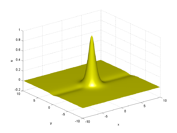
Figure 7: Solution at time $t=4.8\times 10^{-4}$ to the KP-I solution with initial data $\text{sech }^{2}\sqrt{x^{2}+y^{2}}$, which are not subject to the zero mass constraint.

We have already referred to FoSu1 , Su for a rigorous approach to the Cauchy problem with (small) initial data which do not satisfy the zero-mass condition via the Inverse Spectral Method in the integrable case.

Nevertheless, the singularity at $\xi_{1}=0$ of the dispersion relation of KP type equations make them rather bad asymptotic models. First the singularity at $\xi_{1}=0$ yields a very bad approximation of the dispersion relation of the original system (for instance the water wave system) by that of the KP equation.

Another drawback is the poor error estimate between the KP solution and the solution of the original problem. This has been established clearly in the context of water waves (see La ; La2 ; LS ).

The Cauchy problem by PDE techniques

All the KP type equations can be viewed as a linear skew-adjoint perturbation of the Burgers equation. Using this structure, it is not difficult (for instance by a compactness method) to prove that the Cauchy problem is locally well-posed for data in the Sobolev spaces $H^{s}(\mathbb{R}^{2}),$ $s>2$ (see U , Sa , IN for results in this direction).

Unfortunately, this kind of result does not suffice to obtain the global well-posedness of the Cauchy problem. This would need to use the conservation laws of the equations. For general KP type equations, there are only two of them, the conservation of the $L^{2}$ norm and the conservation of the energy (Hamiltonian). For the general equation (46) where $f(u)=\frac{1}{p+1}u^{p+1},$ and without the transport term $u_{x}$ (which can be eliminated by a change of variable), we recall that the Hamiltonian reads

$$E(u)=\frac{1}{2}\int\left[-u\,Lu+(\partial_{x}^{-1}u_{y})^{2}+\frac{u^{p+2}}{p+2}\right],$$ (56)

and for the classical KP I/II equations

$$E(u)=\frac{1}{2}\int\left[u_{x}^{2}\pm(\partial_{x}^{-1}u_{y})^{2}-\frac{u^{3}}{3}\right],$$ (57)

where the $+$ sign corresponds to KP I and the $-$ sign to KP II.

We recall that the “integrable" KP I and KP II equations possess more conservation laws, but only a finite number of them make sense rigorously (see above).

In any case, it is clear that for KP II type equation, the Hamiltonian is useless to control any Sobolev norm, and to obtain the global well-posedness of the Cauchy problem one should consider $L^{2}$ solutions, a very difficult task. On the other hand, for KP I type equations, one may hope (for a not too strong nonlinearity) to have a global control in the energy space, that is

$$E=\{u\in L^{2},\;uLu\in L^{2},\;\partial_{x}^{-1}u_{y}\in L^{2}\}.$$ (58)

For the usual KP I equation, $E$ reduces to

$$Y=\{u\in L^{2},\;u_{x}\in L^{2},\;\partial_{x}^{-1}u_{y}\in L^{2}\}.$$

The problem is thus reduced to proving the local well-posedness of the Cauchy problem in spaces of very low regularity, a difficult matter which has attracted a lot of efforts in the recent years.

Remark 14

By a standard compactness method, one obtains easily the existence of global weak finite energy solutions (without uniqueness) to the KP I equation (see eg Tom ).

A fundamental step for KP II is made in Bourgain who proved that the Cauchy problem for the KP II equation is locally (thus globally in virtue of the conservation of the $L^{2}$ norm) for data in $L^{2}(\mathbb{R}^{2}),$ and even in $L^{2}(\mathbb{T}^{2}).$ This result is based on an iterative method implemented on the Duhamel formulation, in the functional framework of the Fourier restriction $X^{s,b}$ spaces of Bourgain (see a nice description of this framework in Gi ). The basic bilinear estimate which aims to regain the loss of one $x$-derivative uses in a crucial way the fact (both in the periodic and full space case) that the dispersion relation of the KP II equation induces the triviality of a resonant set (the zero set of the aforementioned resonant function). With in particular the injection of various linear dispersive estimates (see for instance Sa ; BAS ), Bourgain’s result was later improved (see TaTz , IM , Ha , HHK and the references therein) to allow the case of initial data in negative order Sobolev spaces.

We also would like to mention the paper by Kenig and Martel KM where the Miura transform is used to prove the global well-posedness of a modified KP II equation.

Moreover it was proven in MST5 that the Cauchy problem for KP II is globally well-posed with initial data

$$u(0,x,y)=\phi(x,y)+\psi_{c}(x,y),$$ (59)

where $\psi_{c}$ is the profile of a non-localized (i.e. not decaying in all spatial directions) traveling wave of the KP II equation moving with speed $c\neq 0$.

We recall (deBS ) that, contrary to the KP I equation, the KP II equation does not possess any localized in both directions traveling wave solution.

The background solution $\psi_{c}$ could be for instance the line soliton (1-soliton) of the Korteweg- de Vries (KdV) equation

$$s_{c}(x,y)=\frac{3c}{2}\,{\rm cosh}^{-2}\Big{(}\frac{\sqrt{c}\,x}{2}\Big{)},$$ (60)

or the N-soliton solution of the KdV equation, $N\geq 2.$

The KdV N-soliton is of course considered as a two dimensional (constant in $y$) object.

There are two suitable settings for an initial perturbation $\phi$, either localized in $x$ and periodic in $y$ (eg $\phi\in L^{2}(\mathbb{R}\times\mathbb{T})$) or localized (eg $\phi\in L^{2}(\mathbb{R}^{2}).)$

Solving the Cauchy problem in both those functional settings can be viewed as a preliminary step towards the study of the dynamics of the KP II equation on the background of a non fully localized solution, in particular towards a PDE proof of the nonlinear stability of the KdV soliton or N-soliton with respect to transversal perturbations governed by the KP II flow. This has been established in AV2 Proposition 17 by Inverse Scattering methods. The advantage of the PDE approach is that it can be straightforwardly applied to non integrable equations such as the higher order KP II equations (see ST2 , ST3 ).

We now state the main result of MST5 in the two aforementioned functional settings.

Theorem 4.3

The Cauchy problem associated with the KP II equation is globally well-posed in $H^{s}(\mathbb{R}\times\mathbb{T})$ for any $s\geq 0$.

Theorem 4.4

Let $\psi_{c}(x-ct,y)$ be a solution of the KP II equation such that for some $s\geq 0$,

$$J^{s}\psi_{c}\,:\,\mathbb{R}^{2}\longrightarrow\mathbb{R}$$

is bounded and belongs to $L^{2}_{x}L^{\infty}_{y}$ . Then for every $\phi\in H^{s}(\mathbb{R}^{2})$ there exists a unique global solution $u$ of KP II with initial data (59) satisfying for all $T>0$,

$$[u(t,x,y)-\psi_{c}(x-ct,y)]\in X^{1/2+,s}_{T}\cap X^{3/4+,s}_{T}\cap C([0,T];H^{s}(\mathbb{R}^{2})).$$

Furthermore, for all $T>0$, the map $\phi\mapsto u$ is continuous from $H^{s}(\mathbb{R}^{2})$ to $C([0,T];H^{s}(\mathbb{R}^{2})))$.

Remark 15

As was previously noticed, the hypothesis on $\psi_{c}$ in Theorem 4.4 is satisfied by the N-soliton solutions of the KdV equation, but not by a function $\psi$ which is non-decaying along a line $\{(x,y)|x-vy=x_{0}\},$ as for instance the line-soliton of the KP II equation which has the form $\psi(x-vy-ct).$

However, the change of variables $(X=x,Y=x-vy)$ transforms the KP II equation into

$$u_{t}-2vu_{Y}+v^{2}u_{X}+u_{XXX}+uu_{X}+\partial_{X}^{-1}u_{YY}=0$$

and the analysis applies to this equation with aninitial datum which is a localized (in $(X,Y)$) perturbation of $\psi(X).$

As was previously mentioned the Cauchy problem for the KP I cannot be solved by a Picard iteration on the integral formulation and one has to implement instead sophisticated compactness methods to obtain the local well-posedness and to use the conservation laws to get global solutions.

For the classical KP I equation, the first global well-posedness result for arbitrary large initial data in a suitable function space was obtained in MST2 in the space

$$Z=\{\phi\in L^{2}(\mathbb{R}^{2})~{}:~{}\|\phi\|_{Z}<\infty\},$$

where

$$\|\phi\|_{Z}=|\phi|_{2}+|\phi_{xxx}|_{2}+|\phi_{y}|_{2}+|\phi_{xy}|_{2}+|\partial_{x}^{-1}\phi_{y}|_{2}+|\partial_{x}^{-2}\phi_{yy}|_{2}.$$

By an anisotropic Sobolev embedding theorem (cf. bes ) if $\phi\in Z$ then $\phi,\phi_{x}\in L^{\infty}(\mathbb{R}^{2}),$ so the global solution is uniformly bounded in space and time. Moreover, if $\phi\in Z$ then the first three formal invariants $M(\phi),E(\phi),F(\phi)$ are well defined and conserved. Furthermore it is easily checked that any finite energy solitary waves (in particular the lumps, see below) of the KP I equation belong to $Z$.

The proof is based on a rather sophisticated compactness method and uses the first invariants of the KP I equation to get global in time bounds. As already mentioned, only a small number of the formal invariants make sense and in order to control $|\phi_{xxx}|_{2}$ one is thus led to introduce a quasi-invariant (by skipping the non well defined terms) which eventually will provide the desired bound. There are also serious technical difficulties to justify rigorously the conservation of the meaningful invariants along the flow and to control the remainder terms

The result of MST2 was extended by Kenig K (who considered initial data in a larger space), and by Ionescu, Kenig and Tataru IKT who proved that the KP I equation is globally well-posed in the energy space $Y$.

Moreover it is proven in MST3 that the Cauchy problem for the KP I equation is globally well-posed for initial data which are localized perturbations (of arbitrary size) of a non-localized i.e. not decaying in all directions) traveling wave solution (e.g. the KdV line solitary wave or the Zaitsev solitary waves which are localized in $x$ and $y$ periodic or conversely (see Section 4.2 below).

Long time behavior

The results above do not give information on the behavior of the global solution for large time. Actually no result in this direction is known by PDE techniques. However, one can make precise the large time behavior of small solutions to the generalized KP equations (46) when $r\geq 2$.

Actually, it is shown in HNS ; Ni that for initial data small in an appropriate weighted Sobolev space, (46) for $r\geq 2$ has a unique global solution satisfying

$$|u(.,t)|_{\infty}\leq C(1+|t|)^{-1}(\text{Log}(1+|t|))^{\kappa},$$

$$|\partial_{x}u(.,t)|_{\infty}\leq C(1+|t|)^{-1},$$

where $\kappa=1$ when $r=2$ and $\kappa=0$ when $r>2.$

This result does not distinguish between the KP I and KP II case since it relies on the (same) large time asymptotic of the KP I and KP II groups $S_{\pm}(t)=e^{it(-\partial_{x}^{3}\pm\partial{-1}_{x}\partial_{y}^{2})},$ namely (see Sa )

$$|S_{\pm}(t)\phi|_{\infty}\leq\frac{C}{|t|}|\phi|_{1}.$$

Remark 16

Since this phenomena does not happen for the classical KP I and KP II equation, we do not comment on the possible blow-up in finite time of solutions to the generalized KP I equation (46) when $r\geq\frac{4}{3}.$ We refer to Liu for a theoretical study and to KP2 ; KS2 for numerical simulations.

4.3 Solitary waves

We are interested here in localized solitary wave solutions to the KP equations, that is solutions of KP equations of the form

$$u(x,y,t)=\psi_{c}(x-ct,y),$$

where $y$ is the transverse variable and $c>0$ is the solitary wave velocity.

The solitary wave is said to be localized if $\psi_{c}$ tends to zero at infinity in all directions. For such solitary waves, the energy space $Y$ is natural. Recall that

$$Y=Y(\mathbb{R}^{2})=\{u\in L^{2}(\mathbb{R}^{2}),\;u_{x}\in L^{2}(\mathbb{R}^{2}),\;\partial_{x}^{-1}u_{y}\in L^{2}(\mathbb{R}^{2})\},$$

and throughout this section we will deal only with finite energy solitary waves.

Due to its integrability properties, the KP I equation possesses a localized, finite energy, explicit solitary wave, the lump:

$$\phi_{c}(x-ct,y)=\frac{8c(1-\frac{c}{3}(x-ct)^{2}+\frac{c^{2}}{3}y^{2})}{(1+\frac{c}{3}(x-ct)^{2}+\frac{c^{2}}{3}y^{2})^{2}}.$$ (61)

The formula was found in MZBM where one can also find a study of the interaction of lumps. The interactions do not result in a phase shift as in the case of line solitons (KdV solitons). More general rational solutions of the KPI equation were subsequently found (Kr ; SatAb ; PeSt ; Pel ; Sat ). These solutions were incorporated within the framework of the IST in VA where it was observed that, in general, the spectral characterization of the potential must include, in addition to the usual information about discrete and continuous spectrum, an integer-valued topological quantity (the index or winding number), defined by an appropriate two-dimensional integral involving both the solution of the KP equation and the corresponding scattering eigenfunction.

Another interesting explicit solitary wave of the KP I equation which is localized in $x$ and periodic in $y$ has been found by Zaitsev Zai . It reads

$$Z_{c}(x,y)=12\alpha^{2}\frac{1-\beta\cosh(\alpha x)\cos(\delta y)}{[\cosh(\alpha x)-\beta\cos(\delta y)]^{2}},$$ (62)

where

$$(\alpha,\beta)\in(0,\infty)\times(-1,+1),$$

and the propagation speed is given by

$$c=\alpha^{2}\frac{4-\beta^{2}}{1-\beta^{2}}.$$

Let us observe that the transform $\alpha\rightarrow i\alpha$, $\delta\rightarrow i\delta$, $c\rightarrow ic$ produces solutions of the KP I equation which are periodic in $x$ and localized in $y$.

No real non-singular rational solutions are known for KP II. Moreover, it was established in deBS that no localized solitary waves exist for the KP II equation (and generalized KP II equations).

For obvious (stability) issues it is important to characterize the solitary waves by variational principles. We will consider in fact the slightly more general class of generalized KP I equations

$$u_{t}+u_{x}+u^{r}u_{x}+u_{xxx}-\partial_{x}^{-1}u_{yy}=0,\;(x,y)\in\mathbb{R}^{2},\;t\geq 0,$$ (63)

where again $r\in\mathbb{N}$ or $r=\frac{p}{q},$ $p,q$ relatively prime integers, $q$ odd.

Solitary waves are looked for in the energy space $Y(\mathbb{R}^{2})$ which can also be defined (see deBS ) as the closure of the space of $x$ derivatives of smooth and compactly supported functions in $\mathbb{R}^{2}$ for the norm

$$\|\partial_{x}f\|_{Y(\mathbb{R}^{2})}\equiv\Big{(}\|\nabla f\|_{L^{2}(\mathbb{R}^{2})}^{2}+\|\partial_{x}^{2}f\|_{L^{2}(\mathbb{R}^{2})}^{2}\Big{)}^{\frac{1}{2}}.$$

The equation of a solitary wave $\psi$ of speed $c$ is given by

$$c\partial_{x}\psi-\psi\partial_{x}\psi-\partial_{x}^{3}\psi+\partial_{x}^{-1}(\partial_{y}^{2}\psi)=0,$$ (64)

which implies

$$c\partial_{xx}\psi-(\psi\partial_{x}\psi)_{x}-\partial_{x}^{4}\psi+\partial_{y}^{2}\psi=0,$$ (65)

When $\psi\in Y(\mathbb{R}^{2})$, the function $\partial_{x}^{-1}\partial_{y}^{2}\psi$ is well-defined (see deBS ), so that (64) makes sense.

Given any $c>0$, a solitary wave $\psi_{c}$ of speed $c$ is deduced from a solitary wave $\psi_{1}$ of velocity $1$ by the scaling

$$\psi_{c}(x,y)=c\psi_{1}(\sqrt{c}x,cy).$$ (66)

We now introduce the important notion of ground state solitary waves.

We set

$$E_{KP}(\psi)=\frac{1}{2}\int_{\mathbb{R}^{2}}(\partial_{x}\psi)^{2}+\frac{1}{2}\int_{\mathbb{R}^{2}}(\partial_{x}^{-1}\partial_{y}\psi)^{2}-\frac{1}{2(p+2)}\int_{\mathbb{R}^{2}}\psi^{p+2},$$

and we define the action

$$S(N)=E_{KP}(N)+\frac{c}{2}\int_{\mathbb{R}^{2}}N^{2}.$$

We call ground state, a solitary wave $N$ which minimizes the action $S$ among all finite energy non-constant solitary waves of speed $c$ (see deBS for more details).

It was proven in deBS that ground states exist if and only if $c>0$ and $1\leq p<4$. Moreover, when $1\leq p<\frac{4}{3},$ the ground states are minimizers of the Hamiltonian $E_{KP}$ with prescribed mass ($L^{2}$ norm).

Remark 17

When $p=1$ (the classical KP I equation), we should emphasize that it is unknown (but conjectured) whether the lump solution is a ground state. This important issue is of course related to the uniqueness of the ground state or of localized solitary waves, up to symmetries. A similar question stands for the focusing nonlinear Schrödinger equation but it can be solved there because the ground state is shown to be radial and and uniqueness follows from (non trivial!) ODE arguments (see Kw ). Of course such arguments cannot work in the KP I case since the lump (or the ground states) are not radial.

It turns out that qualitative properties of solitary waves which are that of the lump solution can be established for a large class of KP type equations. Ground state solutions are shown in deBS2 to be cylindrically symmetric, that is radial with respect to the transverse variable up to a translation of the origin.

On the other hand, any finite energy solitary wave is infinitely smooth (at least when the exponent $p$ is an integer) and decays with an algebraic rate $r^{-2}$ deBS2 . Actually the decay rate is sharp in the sense that a solitary wave cannot decay faster that $r^{-2}.$

Moreover a precise asymptotic expansion of the solitary waves has been obtained by Gravejat (Gra ).

Remark 18

The fact whether the ground states are or are not minimizers of the Hamiltonian is strongly linked to the orbital stability of the set $\mathcal{G}_{c}$ of ground states of velocity $c$. We recall that the uniqueness, up to the obvious symmetries, of the ground state of velocity $c$ is a difficult open problem, even for the classical KP I equation.

Saying that $\mathcal{G}_{c}$ is orbitally stable in $Y$ means that for $\phi_{c}\in\mathcal{G}_{c},$ then for all $\epsilon>0,$ there exists $\delta>0$ such that if $u_{0}\in Y$ is such that $||u_{0}-\phi_{c}||_{Y}\leq\delta,$ then the solution $u(t)$ of the Cauchy problem initiating from $u_{0}$ satisfies

$$\sup_{t\geq 0}\inf_{\psi\in\mathcal{G}}||u(t)-\psi||_{Y}\leq\epsilon.$$

Of course, the previous inequality makes full sense only if one knows that the Cauchy problem is globally well-posed. As we have previously seen, this is the case for the classical KP I equation MST3 , even in the energy space IKT , but is still an open problem for the generalized KP I equation when $1<p<4/3.$

Actually it is proved in deBS3 that the ground state solitary waves of the generalized KP I equations (63) are orbitally stable in dimension two if and only if $1\leq p<\frac{4}{3}$.

4.4 Transverse stability of the line soliton

The KP I and KP II equations behave quite differently with respect to the transverse stability of the KdV $1$-soliton.

Zakharov Za has proven, by exhibiting an explicit perturbation using the integrability, that the KdV $1$-soliton is nonlinearly unstable for the KP I flow. Rousset and Tzvetkov RT1 ; RT2 ; RT3 have given an alternative proof of this result, which does not use the integrability, and which can thus be implemented on other problems (eg for nonlinear Schrödinger equations).

The nature of this instability is not known (rigorously) and one has to rely on numerical simulations (KS2 ; PeSt2 ).

On the other hand, Mizomachi and Tzvetkov MiTz have recently proved the $L^{2}(\mathbb{R}\times\mathbb{T})$ orbital stability of the KdV $1$-soliton for the KP II flow. The perturbation is thus localized in $x$ and periodic in $y$. The proof involves in particular the Miura transform used in KM to established the global well-posedness for a modified KP II equation.

Such a result is not known (but expected) for a perturbation which is localized in $x$ and $y$.

The transverse stability of the KdV soliton has been numerically studied in KS2 from which the figures in this subsection are taken. We considered perturbations of the form

$$u_{p}=6(x-x_{1})\exp(-(x-x_{1})^{2})\left(\exp(-(y+L_{y}\pi/2)^{2})+\exp(-(y-L_{y}\pi/2)^{2})\right),$$ (67)

which are in the Schwartz class for both variables and satisfy the zero mass constraint. They are of the same order of magnitude as the KdV soliton, i.e., of order $0(1)$, and thus test the nonlinear stability of the KdV soliton. As discussed in KS2 , the computations are carried out in a doubly periodic setting, i.e., $\mathbb{T}^{2}$ and not on $\mathbb{R}^{2}$.

For KP II we consider the initial data $u_{0}(x,y)=12\mbox{sech}^{2}(x+2L_{x})-u_{p}$ ($x_{1}=x_{0}/2$), i.e., a superposition of the KdV soliton and the not aligned perturbation which leads to the situation shown in Fig. 8. The perturbation is dispersed in the form of tails to infinity which reenter the computational domain because of the imposed periodicity. The soliton appears to be unaffected by the perturbation which eventually seems to be smeared out in the background of the soliton.

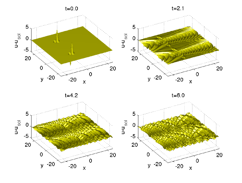
Figure 8: Difference of the solution to the KP II equation for initial data given by the KdV soliton plus perturbation, $u(0,x,y)=u_{sol}(x+2L_{x},0)$ and perturbation $u_{p}=6(x-x_{1})\exp(-(x-x_{1})^{2})\left(\exp(-(y+L_{y}\pi/2)^{2})+\exp(-(y-L_{y}\pi/2)^{2})\right)$, $x_{1}=-L_{x}$ and the KdV soliton for various values of $t$.

The situation is somewhat different if the perturbation and the initial soliton are centered around the same $x$-value initially, i.e., the same situation as above with $x_{1}=x_{0}=-2L_{x}$. In Fig. 9 we show the difference between the numerical solution and the KdV soliton $u_{sol}$ for several times for this case.

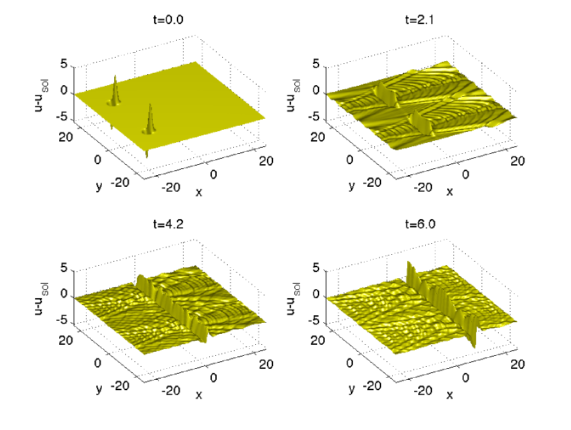
Figure 9: Difference of the solution to the KP II equation for initial data given by the KdV soliton $u_{sol}(x+2L_{x},0)$ plus perturbation $u_{p}=6(x-x_{1})\exp(-(x-x_{1})^{2})\left(\exp(-(y+L_{y}\pi/2)^{2})+\exp(-(y-L_{y}\pi/2)^{2})\right)$, $x_{1}=-2L_{x}$, and the KdV soliton for various values of $t$.

It can be seen that the initially localized perturbations spread in $y$-direction, i.e., orthogonally to the direction of propagation and take finally themselves the shape of a line soliton. It appears that the perturbations lead eventually to a KdV soliton of slightly higher mass. As discussed in KS2 , different types of perturbation all indicate the stability of the KdV soliton for KP II.

It was shown in RT1 ; RT2 ; RT3 ; Za that the KdV soliton is nonlinearly unstable against transversal perturbations in the KP I setting if its mass is above a critical value. The proof in Za relies on the integrability of the KP I equation, but the methods in RT1 ; RT2 ; RT3 apply to general dispersive equations.

However, the type of the instability is unknown. Therefore in KS2 , this question was addressed numerically. In Fig. 10 we show the KP I solution for the perturbed initial data of a line soliton with the perturbation (67) and $x_{1}=x_{0}=-2L_{x}$, i.e., the same setting as studied in Fig. 9 for KP II. Here the initial perturbations develop into 2 lumps which are traveling with higher speed than the line soliton. The formation of these lumps essentially destroys the line soliton which leads to the formation of further lumps. It appears plausible that for sufficiently long times one would only be able to observe lumps and small perturbations which will be radiated to infinity if studied on $\mathbb{R}^{2}$.

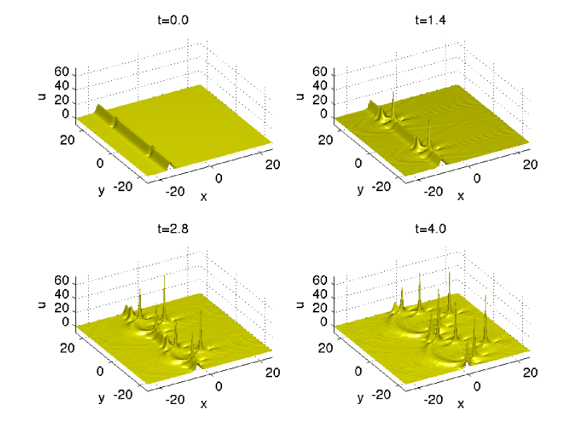
Figure 10: Solution to the KP I equation for initial data given by the KdV soliton $u_{sol}(x+2L_{x},0)$ plus perturbation $u_{p}=6(x-x_{1})\exp(-(x-x_{1})^{2})\left(\exp(-(y+L_{y}\pi/2)^{2})+\exp(-(y-L_{y}\pi/2)^{2})\right)$, $x_{1}=-2L_{x}$, for various values of $t$.

We can give some numerical evidence for the validity of the interpretation of the peaks in Fig. 10 as lumps in an asymptotic sense. We can identify numerically a certain peak, i.e., obtain the value and the location of its maximum. With these parameters one can study the difference between the KP solution and a lump with these parameters to see how well the lump fits the peak. This is illustrated for the two peaks, which formed first and which have therefore traveled the largest distance in Fig. 11.

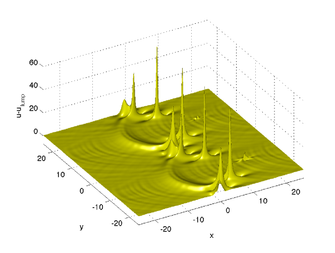
Figure 11: Difference of the solution to the KP I equation in Fig. 10 for $t=4$ and two lump solutions fitted at the peaks farthest to the right. Only very small peaks remain of these ‘lumps’ indicating that they develop asymptotically into true lumps.

A multi-lump solution might be a better fit, but here we mainly want to illustrate the concept which obviously cannot fully apply at the studied small times. Nonetheless Fig. 11 illustrates convincingly that the observed peaks will asymptotically develop into lumps.

Further examples for the nonlinear instability of the KdV soliton in this setting are given in KS2 . However, the nonlinear stability discussed in RT1 ; RT2 can be seen in Fig. 12 where the KP I solution is given for a perturbation of the line soliton as before $u_{0}(x,y)=12\mbox{sech}^{2}(x+2L_{x})+u_{p}$, but this time with $x_{1}=x_{0}/2$, i.e., perturbation and soliton are well separated.

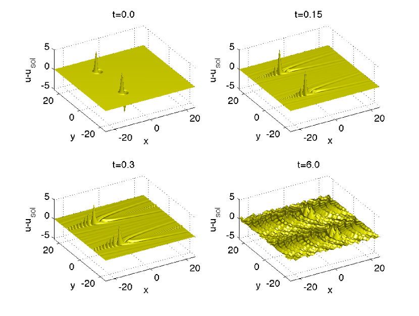
Figure 12: Difference of the solution to the KP I equation for initial data given by the KdV soliton $u_{sol}(x+2L_{x},0)$ plus perturbation $u_{p}=6(x-x_{1})\exp(-(x-x_{1})^{2})\left(\exp(-(y+L_{y}\pi/2)^{2})+\exp(-(y-L_{y}\pi/2)^{2})\right)$, $x_{1}=-L_{x}$ and the KdV soliton for various values of $t$.

The figure shows the difference between KP I solution and line soliton. It can be seen that the soliton is essentially stable on the shown time scales. The perturbation leads to algebraic tails towards positive $x$-values and to dispersive oscillations as studied in KSM2 . Due to the imposed periodicity both of these cannot escape the computational domain and appear on the respective other side. The important point is, however, that though the oscillations of comparatively large amplitude hit the line soliton quickly after the initial time, its shape is more or less unaffected till $t=6$. The KdV soliton eventually decomposes into lumps once it comes close to the boundaries of the computational domain, but this appears to be a numerical effect related to the imposed periodicity in $x$.

5 The Davey-Stewartson systems

The Davey-Stewartson (DS) systems are derived as asymptotic models in the so-called modulation regime from various physical situations (water waves, plasma physics, ferromagnetism, see DS ; AS ; Co ; Le ). They provide also a good approximate solution to general quadratic hyperbolic systems using diffractive geometric optics Co ; CoLa . They have the general form, where $a,b,c,\nu_{1},\nu_{2}$ are real parameters depending on the physical context

$$\begin{array}[]{ccc}i\partial_{t}\psi+a\partial_{x}^{2}\psi+b\partial_{y}^{2}\psi=(\nu_{1}|\psi|^{2}+\nu_{2}\partial_{x}\phi)\psi,\\ \partial_{x}^{2}\phi+c\partial_{y}^{2}\phi=-\delta\partial_{x}|\psi|^{2},\end{array}$$ (68)

where one can assume (up to a change of unknown) $a>0$ and $\delta>0.$

Using the terminology of GS , one says that (68) is

elliptic-elliptic if  ($\text{sgn}\;b,\text{sgn}\;c)=(+1,+1),$

hyperbolic-elliptic if  ($\text{sgn}\;b,\text{sgn}\;c)=(-1,+1),$

elliptic-hyperbolic if  ($\text{sgn}\;b,\text{sgn}\;c)=(+1,-1),$

hyperbolic-hyperbolic if  ($\text{sgn}\;b,\text{sgn}\;c)=(-1,-1).$

It is worth noticing that the Davey-Stewartson systems are "degenerate" versions of a more general class of systems describing the interaction of short and long waves, the Benney-Roskes, Zakharov-Rubenchik systems (BR ; ZR ). None of those systems is known to be integrable.

It turns out that a very special case of the hyperbolic-elliptic and the elliptic-hyperbolic DS systems are completely integrable. They are then classically known respectively as the DS II and DS I systems. Since we want to compare IST and PDE methods, we will focus on the hyperbolic-elliptic and elliptic-hyperbolic cases (referred to as DS II type and DS I type). We refer to GS ; Ci ; Ci2 for results on the elliptic-elliptic DS systems.

We will from now on write the DS II system in the form

$$\begin{array}[]{ccc}i\partial_{t}\psi+\partial_{xx}\psi-\partial_{yy}\psi+2\rho\left(\beta\Phi+\left|\psi\right|^{2}\right)\psi&=&0,\quad\psi:\mathbb{R}^{2}\times\mathbb{R}\to\mathbb{C},\\ \partial_{xx}\Phi+\partial_{yy}\Phi+2\partial_{xx}\left|\psi\right|^{2}&=&0,\quad\Phi:\mathbb{R}^{2}\times\mathbb{R}\to\mathbb{R},\\ \psi(.,0)=\psi_{0},\end{array}$$ (69)

where the integrable DS II system corresponds to $\beta=1$ and $\rho$ takes the values $-1$ (focusing) and $1$ (defocusing).

The DS II system can be viewed as a nonlocal cubic nonlinear Schrödinger equation. Actually one can solve $\Phi$ as

$$\Phi=2[(-\Delta)^{-1}\partial_{xx}]|\psi|^{2},$$

where $(-\Delta)^{-1}\partial_{xx}=R_{1}^{2}$ is a zero order operator with Fourier symbol $-\frac{\xi_{1}^{2}}{|\xi|^{2}}$ and is thus bounded in all $L^{p}(\mathbb{R}^{2})$ spaces, $1<p<\infty$ and all Sobolev spaces $H^{s}(\mathbb{R}^{2}),$ allowing to write (69) as

$$i\partial_{t}\psi+\partial_{xx}\psi-\partial_{yy}\psi+2\rho\left(2\beta R_{1}^{2}(|\psi|^{2})+\left|\psi\right|^{2}\right)\psi=0.$$ (70)

One easily finds that (69) has two formal conservation laws, the $L^{2}$ norm

$$\int_{\mathbb{R}^{2}}|\psi(x,y,t)|^{2}dxdy=\int_{\mathbb{R}^{2}}|\psi(x,y,0)|^{2}dxdy$$

and the energy (Hamiltonian)

$$E(\psi(t)) = \int_{\mathbb{R}^{2}}\left[|\partial_{x}\psi|^{2}-|\partial_{y}\psi|^{2}-\rho(|\psi|^{2}+\beta\Phi)|\psi|^{2})\right]dxdy$$ (71)

$$= E(\psi(0)).$$

Note that the integrable case $\beta=1$ is distinguished by the fact that the same hyperbolic operator appears in the linear and in the nonlinear part. In this case the equation is invariant under the transformation $x\to y$ and $\psi\to\bar{\psi}$ and (70) can be written in a "symmetric" form as

$$i\partial_{t}\psi+\Box\psi-2\rho[(\Delta^{-1}\Box)|\psi|^{2}]\psi=0,$$ (72)

where $\Box=\partial_{xx}-\partial_{yy}.$

This extra symmetry in the integrable case could be responsible for properties (existence of localized lump solutions and to blow-up phenomena in case of DS II and existence of coherent "dromion" structures in case of DS I) that exist in the integrable case and might not persist in the non integrable cases as the following discussion will suggest.

We summarize now some issues discussed in KS3 where one can also find many numerical simulations.

5.1 DS II type systems

Systems (70) (whatever the value of $\rho$ or $\beta$) can be seen as nonlocal variants of the hyperbolic nonlinear Schrödinger equation

$$i\psi_{t}+\psi_{xx}-\psi_{yy}\pm|\psi|^{2}\psi=0,\quad\psi(\cdot,0)=\psi_{0}$$ (73)

and actually one can obtain (using Strichartz estimates in the Duhamel formulation) exactly the same results concerning the Cauchy problem (see GS ). Namely the Cauchy problem for (70) is locally well-posed for initial data $\psi_{0}$ in $L^{2}(\mathbb{R}^{2})$ or $H^{1}(\mathbb{R}^{2}),$ and globally if $|\psi_{0}|_{2}$ is small enough. Nevertheless, since the existence time does not depend only on $|\psi_{0}|_{2}$ but on $\psi_{0}$ in a more complicated way, one cannot infer from the conservation of the $L^{2}$ norm that the $L^{2}$ solution is a global one. Actually, proving (or disproving) the global well-posedness of the Cauchy problem for (73) is an outstanding open problem.

As for the KP II equation, the inverse scattering problem for the (integrable) DS II is a $\bar{\partial}$ problem.

It turns out that in the integrable case ($\beta=1$) inverse scattering techniques provide far reaching results which seem out of reach of purely PDE methods.

In particular, Sung (Su1 ; Su2 ; Su3 ; Su4 ) has proven the following

Theorem 5.1

Assume that $\beta=1.$ Let $\psi_{0}\in\mathcal{S}(\mathbb{R}^{2}).$ Then (69) possesses a unique global solution $\psi$ such that the mapping $t\mapsto\psi(\cdot,t)$ belongs to $C^{\infty}(\mathbb{R},\mathcal{S}(\mathbb{R}^{2}))$ in the two cases:

(i) Defocusing.

(ii) Focusing and $|\widehat{\psi_{0}}|_{1}|\widehat{\psi_{0}}|_{\infty}<C,$ where $C$ is an explicit constant.

Moreover, there exists $c_{\psi_{0}}>0$ such that

$$|\psi(x,t)|\leq\frac{c_{\psi_{0}}}{|t|},\quad(x,t)\in\mathbb{R}^{2}\times\mathbb{R}^{*}.$$

Remark 19

1. Sung obtains in fact the global well-posedness (without the decay rate) in the defocusing case under the assumption that $\hat{\psi}_{0}\in L^{1}(\mathbb{R}^{2})\cap L^{\infty}(\mathbb{R}^{2})$ and $\psi_{0}\in L^{p}(\mathbb{R}^{2})$ for some $p\in[1,2),$ see Su4 .

2. Recently, Perry Pe has given a more precise asymptotic behavior in the defocusing case for initial data in $H^{1,1}(\mathbb{R}^{2})=\{f\in L^{2}(\mathbb{R}^{2})\;\text{such that}\;\nabla f,(1+|\cdot|)f\in L^{2}(\mathbb{R}^{2})\},$ proving that the solution obeys the asymptotic behavior in the $L^{\infty}(\mathbb{R}^{2})$ norm:

$$\psi(x,t)=u(\cdot,t)+o(t^{-1}),$$

where $u$ is the solution of the linearized problem.

On the other hand, using an explicit localized lump like solution (see below) and a pseudo-conformal transformation, Ozawa Oz has proven that the integrable focusing DS II system possesses an $L^{2}$ solution that blows up in finite time $T^{*}$. In fact the mass density $|\psi(.,t)|^{2}$ of the solution converges as $t\to T^{*}$ to a Dirac measure with total mass $|\psi(.,t)|^{2}_{2}=|\psi_{0}|^{2}_{2}$ (a weak form of the conservation of the $L^{2}$ norm). Every regularity breaks down at the blow-up point but the solution persists after the blow-up time and disperses in the sup norm when $t\to\infty$ as $t^{-2}.$ The numerical simulations in KS suggest that a blow-up in finite time may also happen for other initial data, eg a sufficiently large Gaussian. Other numerical simulations suggest that the finite time blow-up does not persist in the non integrable, $\beta\neq 1$ case, both for the defocusing and focusing cases.

The family of lump solutions (solitons) to the integrable focusing DS II system reads (APP ; MZBM ; AC )

$$\psi(x,y,t)=2c\frac{\exp\left(-2i(\xi x-\eta y+2(\xi^{2}-\eta^{2})t)\right)}{|x+4\xi t+i(y+4\eta t)+z_{0}|^{2}+|c|^{2}}$$ (74)

where $(c,z_{0})\in\mathbb{C}^{2}$ and $(\xi,\eta)\in\mathbb{R}^{2}$ are constants. The lump moves with constant velocity $(-4\xi,-4\eta)$ and decays as $(x^{2}+y^{2})^{-1}$ for $x,y\to\infty$.

As explained in APP , there is a one-to-one correspondence between the lumps and the pole of the matrix solution of the direct scattering problem. It is shown formally in GK and rigorously in Ki that the lump is unstable in the following sense. The soliton structure of the scattering data is unstable with respect to a small compactly supported perturbation of the soliton-like potential. It was also proven in PeSu ; PeSu2 that the lump is spectrally unstable.

The stability of the lump was numerically studied in MFP ; KMR . It was shown that the lump is both unstable against an $L^{\infty}$ blow-up in finite time and against being dispersed away. In Fig. 13 taken from KMR , we consider an initial condition of the form $\psi(x,y,-3)=0.9\psi_{l},$ where $\psi_{l}$ is the lump solution (74) with $c=1$. The solution travels at the same speed as before, but its amplitude varies, growing and decreasing successively.

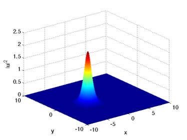
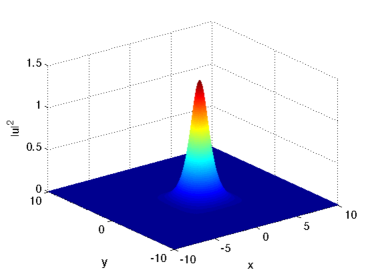
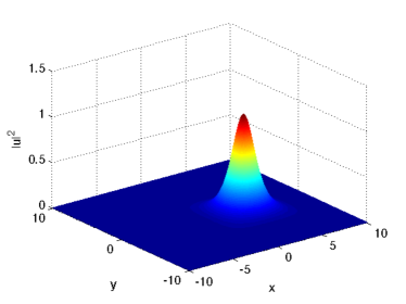
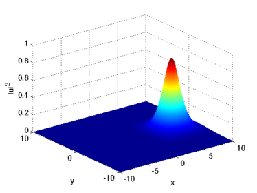
Figure 13: Solution to the focusing DS II equation (69) for an initial condition of the form $\psi(x,y,-3)=0.9\psi_{l}$.

If instead the initial data $\psi(x,y,-3)=0.9\psi_{l},$ is considered, the solution appears to blow up in finite time as can be seen in Fig. 14. Note that also the Ozawa solution Oz was in KMR numerically shown to be unstable against both an earlier blow-up and being dispersed away. In KS3 it was shown that the blow-up of the Ozawa solution is not generic.

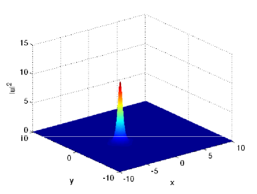
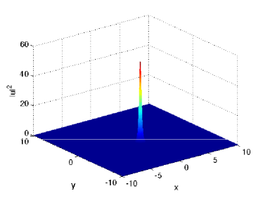
Figure 14: Solution to the focusing DS II equation (69) for an initial condition of the form $\psi(x,y,-3)=1.1\psi_{l}$.

Localized solitary waves of DS II type systems

It is well known that hyperbolic NLS equations such as (73) do not possess solitary waves of the form $e^{i\omega t}\psi(x)$ where $\psi$ is localized (see GS1 ).

It was furthermore proven in GS1 that non trivial solitary waves may exist for DS II type systems only when $\rho=-1$ (focusing case) and $\beta\in(0,2).$ Note that the (focusing) integrable case corresponds to $\beta=1.$ Moreover solitary waves with radial (up to translation) profiles can exist only when $\rho=-1$ and $\beta=1$, that is in the focusing integrable case.

Those results (and the numerical simulations in KMR ; KS ) suggest that localized solitary waves for the focusing DS II systems exist only in the integrable case and this might be due to the new symmetry of the system we were alluding to above in this case.

To summarize, one is led to conjecture that neither the existence of the lump nor the associated Ozawa blow-up persist in the focusing DS II non integrable case. One can also conjecure that the solution of DS II type solution is global and decays in the sup norm as $1/t$ as was shown by Sung and Perry in the (integrable) DS II case.

Remark 20

The previous results and conjectures do not of course exclude the existence of nontrivial, non localized, traveling waves. In the context of the hyperbolic cubic NLS, see for instance Remark 2.1 in GS1 or KNZ . We do not know of existence of similar solutions for DS II type systems.

5.2 DS I type systems

The DS I type systems are quite different from the other DS systems. Actually, solving the hyperbolic equation for $\phi$ (with suitable conditions at infinity) yields a loss of one derivative in the nonlinear term and the resulting NLS type equation is no more semilinear. Even proving the rigorous conservation of the Hamiltonian leads to serious problems. We describe now how to solve the equation for $\phi$ in a $H^{1}$ framework (see GS ).

The elliptic-hyperbolic DS system can be written after scaling as

$$\left\{\begin{aligned} &i\partial_{t}\psi+\Delta\psi=\chi|\psi|^{2}\psi+b\psi\phi_{x}\\ &\phi_{xx}-c^{2}\phi_{yy}=\frac{\partial}{\partial x}|\psi|^{2}.\end{aligned}\right.$$

The integrable DS I system corresponds to $\chi+\frac{b}{2}=0.$

We now solve the equation for $\phi.$

Let $c>0.$ Consider the equation

$$\frac{\partial^{2}\phi}{\partial x^{2}}-c^{2}\frac{\partial^{2}\phi}{\partial y^{2}}=f\quad\text{in}\;\mathbb{R}^{2}$$ (75)

with the boundary condition

$$\lim_{\xi\to+\infty}\phi(x,y)=\lim_{\eta\to+\infty}\phi(x,y)=0$$ (76)

where $\xi=cx-y$ and $\eta=cx+y.$

Let $K=K_{c}$ the kernel

$$K(x,y;x_{1},y_{1})=\frac{1}{2}H(c(x_{1}-x)+y-y_{1})H(c(x_{1}-x)+y_{1}-y)$$

where $H$ is the usual Heaviside function.

Lemma 4

(GS ). For every $f\in L^{1}(\mathbb{R}^{2}),$ the function $\phi=\mathcal{K}(f)$ defined by

$$\phi(x,y)=\int_{\mathbb{R}^{2}}K(x,y;x_{1},y_{1})f(x_{1},y_{1})dx_{1}dy_{1}$$ (77)

is continuous on $\mathbb{R}^{2}$ and satisfies (75) in the sense of distributions. Moreover, $\phi\in L^{\infty}(\mathbb{R}^{2}),(\partial\phi/\partial x)^{2}-c^{2}(\partial\phi/\partial y)^{2}\in L^{1}(\mathbb{R}^{2})$ and we have the following estimates

$$\sup_{(x,y)\in\mathbb{R}^{2}}|\phi(x,y)|\leq\int_{\mathbb{R}^{2}}|f|dxdy$$ (78)

$$\int_{\mathbb{R}^{2}}\left|\left(\frac{\partial\phi}{\partial x}\right)^{2}-c^{2}\left(\frac{\partial\phi}{\partial y}\right)^{2}\right|dxdy\leq\frac{1}{2c}\left(\int_{\mathbb{R}^{2}}|f|dxdy\right)^{2}.$$ (79)

Remark 21

1. No condition is required as $\xi$ or $\eta$ tends to $-\infty.$ 2. In general, $\nabla\phi\notin L^{2}(\mathbb{R}^{2})$ even if $f\in C_{0}^{\infty}(\mathbb{R}^{2}),$ but Lemma 4 allows to solve the $\phi$ equation as soon as $\psi\in H^{1}(\mathbb{R}^{2})$ for instance.

The DS I type system possesses the formal Hamiltonian

$$E(t)=\int_{\mathbb{R}^{2}}\left[|\nabla\psi|^{2}+\frac{\chi}{2}|\psi|^{4}+\frac{b}{2}(\phi_{x}^{2}-c^{2}\phi_{y}^{2})\right]dxdy.$$

Lemma 4 allows to prove that this Hamiltonian makes sense in an $H^{1}$ setting for $\psi$ (see (GS). Proving its conservation on the time interval of the solution is an open problem as far as we know (this would lead to global existence of a weak $H^{1}$ solution).

DS I type by PDE methods

The first local well-posedness result is due to Linares-Ponce LiPo2 and we summarize below the best known results, due to Hayashi-Hirata NH1 ; NH2 and Hayashi H .

After rotation, one can write the DS-I type systems as

$$\left\{\begin{aligned} &i\partial_{t}\psi+\Delta\psi=i(c_{1}+\frac{c_{2}}{2})|\psi|^{2}\psi-\frac{c_{2}}{4}\left(\int_{x}^{\infty}\partial_{y}|\psi|^{2}dx^{\prime}+\int_{y}^{\infty}\partial_{x}|\psi|^{2}dy^{\prime}\right)\psi\\ &+\frac{c_{2}}{\sqrt{2}}\left((\partial_{x}\phi_{1})+\partial_{y}\phi_{2})\right)\psi,\end{aligned}\right.$$

where $c_{1},c_{2}\in\mathbb{R}$ and $\phi$ satisfies the radiation conditions

$$\lim_{y\to\infty}\phi(x,y,t)=\phi_{1}(x,t),\quad\lim_{x\to\infty}\phi(x,y,t)=\phi_{2}(y,t).$$

Theorem 5.2

(H )

Assume $\psi_{0}\in H^{2}(\mathbb{R}^{2}),\;\phi_{1}\in C(\mathbb{R};H^{2}_{x})\;\text{and}\;\phi_{2}\in C(\mathbb{R};H^{2}_{y}).$ Then there exist $T>0$ and a unique solution $\psi\in C([0,T];H^{1})\cap L^{\infty}(0,T;H^{2})$ with initial data $\psi_{0}.$

• The proof uses in a crucial way the smoothing properties of the Schrödinger group.

The next result concerns global existence and scattering of small solutions in the weighted Sobolev space

$$H^{m,l}=\{f\in L^{2}(\mathbb{R}^{2});|(1-\partial_{x}^{2}-\partial_{y}^{2})^{m/2}(1+x^{2}+y^{2})^{l/2}f|_{L^{2}}<\infty\}.$$

Theorem 5.3

(NH2 ) Let $\psi_{0}\in H^{3,0}\cap H^{0,3},\;\partial_{x}^{j+1}\phi_{1}\in C(\mathbb{R};L^{\infty}_{x}),\;\partial_{y}^{j+1}\phi_{2}\in C(\mathbb{R};L^{\infty}_{y}),\;(0\leq j\leq 3),$ "small enough". Then

• There exists a solution $\psi\in L^{\infty}_{\text{loc}}(\mathbb{R};H^{3,0}\cap H^{0,3})\cap C(\mathbb{R};H^{2,0}\cap H^{0,2}).$

• Moreover

  $$||\psi(\cdot,t)||_{L^{\infty}}\leq C(1+|t|)^{-1}(||\psi||_{H^{3,0}}+||\psi||_{H^{0,3}}).$$

  There exist $u^{\pm}$ such that

  $$||\psi(t)-U(t)u^{\pm}||_{H^{2,0}}\to 0,\quad\text{as}\;\to\pm\infty.$$

where $U(t)=e^{it(\partial_{x}^{2}+\partial_{y}^{2}}).$

DS I by IST. Comparison with elliptic-hyperbolic DS

Contrary to the results of the previous subsection which were valid for arbitrary values of $\beta$ we focus here on the integrable case, $\beta=1.$

The first set of results concerns coherent structures (dromions) for DS I with nontrivial conditions (on $\phi$) at infinity. The existence of dromions is established in BLMP ; FoSa and the perturbations of the dromion are investigated in Ki3 (see also Section 7 of Ki ).

We do not know of any study of dromions by PDE techniques or of existence of similar structures in the non-integrable case. Actually they might have no physical relevance.

Concerning the Cauchy problem, the global existence and uniqueness of a solution $\psi\in C(\mathbb{R};\mathcal{S}(\mathbb{R}^{2}))$ of DS I for data $\psi_{0}\in\mathcal{S}(\mathbb{R}^{2}),\;\phi_{1},\phi_{2}\in C(\mathbb{R};\mathcal{S}(\mathbb{R}))$ is proven in FoSu2 . Under a smallness condition, the solutions with trivial boundary conditions $\phi_{1}=\phi_{2}=0$ disperse as $1/t$ (Kiselev Ki3 , see also Ki ). A precise asymptotics is also given. The numerical simulations in BB for general DS I type systems confirm the dispersion of solutions of DS I with trivial boundary conditions and suggest that the dromion is not stable with respect to the coefficients, that is it does not persist in the non-integrable case.

6 Final comments

We briefly comment here on two other integrable equations.

6.1 The Ishimori system

The Ishimori systems were introduced in Ishi as two-dimensional generalizations of the Heisenberg equation in ferromagnetism. They read

$$\begin{array}[]{ccc}S_{t}=S\wedge(S_{xx}-S_{yy})+b(\phi_{x}S_{y}+\phi_{y}S_{x})\\ \phi_{xx}+\phi_{yy}=2S\cdot(S_{x}\wedge S_{y})\\ S(\cdot,0)=S_{0},\end{array}$$ (80)

$$\begin{array}[]{ccc}S_{t}=S\wedge(S_{xx}+S_{yy})+b(\phi_{x}S_{y}+\phi_{y}S_{x})\\ \phi_{xx}-\phi_{yy}=-2S\cdot(S_{x}\wedge S_{y})\\ S(\cdot,0)=S_{0},\end{array}$$ (81)

where $S$ is the spin, $S(\cdot,t):\mathbb{R}^{2}\to\mathbb{R}^{3},$ $|S|^{2}=1,$ $S\to(0,0,1)$ as $|(x,y)|\to\infty$ and $\wedge$ is the wedge product in $\mathbb{R}^{3}.$

The coupling potential $\phi$ is a scalar unknown related to the topological charge density $q(S)=2S\cdot(S_{x}\wedge S_{y}).$ $b$ is a real coupling constant. When $b=1$, (80), (81) are completely integrable (KoMa ; KoMa2 ).

Note the formal analogy of (80), (81) with DS II and DS I type systems.

It is proven in So that the Cauchy problem for (80) (for arbitrary values of $b$) is locally well-posed in $H^{m}(\mathbb{R}^{2}),m\geq 3$ provided the initial spins are almost parallel. Under a stronger regularity assumption on the initial data it is furthermore proven that the solution is global and converges to a solution of the linear "hyperbolic" Schrödinger equation as t goes to infinity.

The idea is to reduce (80), (81) to a nonlinear (hyperbolic) Schrödinger type equation by the stereographic projection

$$u:\mathbb{R}^{2}\to\mathbb{C},\;u=\frac{S^{1}+iS^{2}}{1+S^{3}},$$

reducing (80) to

$$\left\{\begin{array}[]{l}iu_{t}+u_{xx}-u_{yy}=\frac{2\bar{u}}{1+|u|^{2}}(u_{x}^{2}-u_{y}^{2})+ib(\phi_{x}u_{y}+\phi_{x}u_{x})\\ \Delta\phi=4i\frac{u_{x}\bar{u_{y}}-\bar{u_{x}}u_{y}}{(1+|u|^{2})^{2}}\\ u(\cdot,0)=u_{0},\end{array}\right.$$ (82)

with the condition $|u(x,y)|\to 0$ as $|(x,y)|\to\infty.$

The initial condition on $S$ becomes thus a smallness condition on $u_{|t=0}.$

The local well-posedness of the Cauchy problem for (80) for arbitrary initial data in $H^{m}(\mathbb{R}^{2}),m\geq 4$ is proven in KN . This result is improved in BIK where local well-posedness is proven for arbitrary large initial data in $H^{s}(\mathbb{R}^{2}),s>\frac{3}{2}$ having a range that avoids a neighborhood of the north pole.

Concerning the IST method for (80), the rigorous justification of the procedure in KoMa ; KoMa2 is not trivial and Sung Su5 used instead a gauge transform which relates (80) (when $b=1$) to the focusing integrable DS II system. This allows to prove the global well-posedness of the Cauchy problem for small initial data (in a different functional setting than So ).

The connection between the (integrable) Ishimori system (80) is nicely used in BIK to prove the global well-posedness of the Cauchy problem for (80) in the defocusing case, that is when the target of $S$ is no more the sphere $\mathbb{S}^{2}$, but the hyperbolic space $\mathbb{H}^{2}=\{(x,y,z)\in\mathbb{R}^{3};x^{2}-y^{2}-z^{2}=1,x>0\}.$ The gauge transform relates in this case the defocusing Ishimori system (80) to the defocusing DS II system. Such a result is not known in the non integrable case, $b\neq 1.$

We do not know of any finite time blow-up for (80) or of any rigorous result (by PDE or IST methods) for (81).

6.2 The Novikov-Veselov equation

The Novikov-Veselov system

$$\left\{\begin{array}[]{l}v_{t}=4\text{Re}\;(4\partial_{z}^{3}v+\partial_{z}(vw)-E\partial_{z}w),\\ \partial_{\bar{z}}w=-3\partial_{z}v,\quad v=\bar{v}\end{array}\right.$$ (83)

where $\partial_{z}=\frac{1}{2}\left(\partial_{x}-i\partial_{y}\right),\quad\partial_{\bar{z}}=\frac{1}{2}\left(\partial_{x}+i\partial_{y}\right),$

was introduced in NV1 ; NV2 as a two dimensional analog of the Korteweg-de Vries equation, integrable via the inverse scattering transform for the following 2-dimensional stationary Schrödinger equation at a fixed energy $E$:

$$L\psi=E\psi,\quad L=-\Delta+v(x,y,t),$$ (84)

where $\Delta=\frac{\partial^{2}}{\partial x^{2}}+\frac{\partial^{2}}{\partial y^{2}}$ and $E$ is a fixed real constant.

The Novikov-Veselov equation has the Manakov triple representation Ma2

$$\dot{\mathcal{L}}=[A,\mathcal{L}]-B\mathcal{L},$$ (85)

where

$$\mathcal{L}=-\Delta+v+E,$$

$$A=8(\partial^{3}+\bar{\partial^{3}})+2(w\partial+\bar{w}\bar{\partial}),$$

$$\bar{B}=-2(\partial w+\bar{\partial}\bar{w}),$$

that is $(v,w)$ solves (87) if and only if (85) holds.

Remark 22

There is an interesting formal limit of (83) to KP I (resp. KP II) as $E\to+\infty$ (resp. $E\to-\infty)$, under an appropriate scaling, assuming tht the wavelengths in $y$ are much larger than those in $x$.

Remark 23

As far as we know, and contrary to the integrable equations studied above, the Novikov-Veselov equation does not seem be derived as an asymptotic model from a more general system.

To make the equation more "PDE like", we first write the equation in a slightly different form.

Setting $w=w_{1}+iw_{2},$ (83) becomes:

$$\left\{\begin{array}[]{l}v_{t}=2v_{xxx}-6v_{xyy}+2[(vw_{1})_{x}+(vw_{2})_{y}]-2E(\partial_{x}w_{1}+\partial_{y}w_{2}),\;(x,y)\in\mathbb{R}^{2},\;t>0,\\ \partial_{x}w_{1}-\partial_{y}w_{2}=-3v_{x}\\ \partial_{x}w_{2}+\partial_{y}w_{1}=3v_{y}.\end{array}\right.$$ (86)

Note that the last two equations imply

$$(\partial_{xx}-\partial_{yy})w_{2}+2\partial_{xy}w_{1}=0$$

and that $w_{1}$ et $w_{2}$ are defined up to an additive constant.

One can express $w=(w_{1},w_{2})$ in dependence of $v$, in a unique way via the Fourier transform

$$\hat{w_{1}}=\frac{3(\xi_{2}^{2}-\xi_{1}^{2})}{|\xi|^{2}}\hat{v},\quad\hat{w_{2}}=\frac{6\xi_{1}\xi_{2}}{|\xi|^{2}}\hat{v}.$$

We denote $L_{1}$ and $L_{2}$ the zero order corresponding operators,

$$w_{1}=L_{1}v,\quad w_{2}=L_{2}v.$$

With these notations, the equation reads

$$v_{t}-2v_{xxx}+6v_{xyy}+2E(L_{1}v_{x}+L_{2}v_{y})-2[(vL_{1}v)_{x}+(vL_{2}v)_{y}]=0.$$ (87)

One remarks that the dispersive part in (87) is reminiscent of that of the Zakharov-Kuznetzov equation ZR

$$u_{t}+u_{x}+\Delta u_{x}+uu_{x}=0,$$

another two-dimensional extension of the KdV equation, which is not integrable though. We refer to BAKS for a systematic study of the dispersive properties of general third order (local) operators in two-dimensions.

The zero energy case $E=0$.

We refer to the excellent survey CMMPSS for a rather complete account of what is known in this case and which comprises some interesting numerics and a rich bibliography.

We extract from CMMPSS the following definition :

Definition 1

The operator $L=-\Delta+v$ is said to be:

(i) subcritical if the operator $L$ has a positive Green’s function and the equation $L=0$ has a strictly positive distributional solution,

(ii) critical if $L=0$ has a bounded strictly positive solution but no positive Green’s function, and

(iii) supercritical otherwise.

The following conjecture is made in CMMPSS .

Conjecture. The Novikov-Veselov equation with zero energy has a global solution for critical and subcritical initial data, but its solution may blow up in finite time for supercritical initial data.

We refer to CMMPSS for some partial results toward its resolution.

The case $E\neq 0.$

For nonzero energy $E$ and potentials $v$ which vanish at infinity, the scattering transform and inverse scattering method was developed by P. Grinevich, R. G. Novikov, and S.-P. Novikov (see Kazeykina’s thesis Kaz for an excellent survey and Gr2 ; GrMa ; GrNo for the original papers).

We also refer to Kaz and to the papers Kaz1 ; Kaz2 ; Kaz3 ; KaNo1 ; KaNo2 ; KaNo3 ; Nov for many interesting results on the soliton solutions (absence, decay properties,..) and the long time asymptotics. More precisely it is proven that the rational, non singular solutions introduced in Gr2 ; Gr3 at positive energy are multi-solitons. It is also proven that solitons cannot decay faster than $O(|x|^{-3})$ when $E\neq 0$ and than $O(|x|^{-2})$ when $E=0.$ Finally, the evolution solutions corresponding to non singular scattering data are shown to decay asymptotically as $O(t^{-1})$ when $E>0$ and as $O(t^{-3/2})$ when $E<0.$

Novikov-Veselov by PDE techniques

We only know of one result on Novikov-Veselov by PDE techniques. Angelopoulos Ang has proven the local well-posedness in $H^{1/2}(\mathbb{R}^{2})$ of the Cauchy problem in the zero energy case ($E=0$) case following the method used in MP2 . It is very likely that the methods in KoSa for the Zakharov-Kuznetsov equation would lead to a local well-posedness result when $E\neq 0,$ not in the "optimal" space though.

Note than one cannot perform simple energy estimates on (87) (as in the KP or Zakharov-Kuznetsov case) leading "for free" to a local result in $H^{s}(\mathbb{R}^{2}),s>2$ (actually even the $L^{2}$ estimate on (87) fails).

Also PDE methods should solve the aforementioned problem of the "long wave" KP limit when $E\to\pm\infty.$ Actually similar questions are already solved for the Gross-Pitaevskii equation (see CR ; BGSS1 ; BGSS2 ).

Finally we do not know of any stability results (by PDE methods) for the Novikov-Veselov solitary waves.

Acknowledgement:
The Authors thank Anne de Bouard, Anna Kazeykina, Thanasis Fokas, Oleg Kiselev and P. Perry for fruitful conversations. J.-C. S. was partially supported by the project GEODISP of the Agence Nationale de la Recherche.

References

- (1) L. Abdelouhab, J. Bona, M. Felland and J.-C.Saut, Non local models for nonlinear dispersive waves, Physica D Nonlinear Phenomena, 40, (1989), 360-392.
- (2) M.J. Ablowitz and P.A. Clarkson, Solitons, nonlinear evolution equations and inverse scattering, London Mathematical Society Lecture Notes series 149, Cambridge University Press, (1991).
- (3) M.J. Ablowitz and A.S. Fokas, The inverse scattering transform for the Benjamin-Ono equation : a pivot to multidimensional problems, Stud; App. Math. 68 (1983), 1-10.
- (4) M.J. Ablowitz and H. Segur, On the evolution of packets of water waves, J. Fluid Mech. 92 (1979), 691-715.
- (5) M. J. Ablowitz, J. Villarroel, The Cauchy problem for the Kadomtsev-Petviashvili II equation with with nondecaying data along a line, Studies Appl. Math 109 (2002), 151-162.
- (6) M. J. Ablowitz, J. Villarroel, The Cauchy problem for the Kadomtsev-Petviashvili II equation with data that do not decay along a line, Nonlinearity 17 (2004), 1843-1866.
- (7) J. P. Albert and J. L. Bona, Total Positivity and the Stability of Internal Waves in Stratified Fluids of Finite Depth IMA J. Appl. Math. 46 (1-2) (1991), 1-19.
- (8) J.P. Albert, J. L Bona and D. Henry,Sufficient conditions for stability of solitary-wave solutions of model equations for long waves, Physica D 24, (1987), 343-366.
- (9) J.P. Albert, J.L. Bona and N.V. Nguyen, On the stability of KdV multi-solitons, Diff. Int. Equations 20 (8) (2007), 841-878.
- (10) J.P.Albert and J.F. Toland, On the exact solutions of the intermediate long-wave equation, Diff. Int. Eq. 7 (3-4) (1994), 601-612.
- (11) C.J. Amick and J. Toland, Uniqueness and related analytic properties for the Benjamin-Ono equation-a nonlinear Neumann problem in the plane, Acta Math. 167 (1991), 107-126.
- (12) R.L. Anderson and E. Taflin, The Benjamin-Ono equation-Recursivity of linearization maps-Lax pairs, Letters Math. Phys. 9 (1985), 299-311.
- (13) Y. Angelopoulos, Well-posedness and ill-posedness results for the Novikov-Veselov equation, arXiv 1307.4110 (2013).
- (14) V.A. Arkadiev, A.K. Pogrebkov and M.C. Polivanov, Inverse scattering transform and soliton solution for Davey-Stewartson II equation, Physica D 36 (1089), 188-197.
- (15) R. Beals and R.R. Coifman,Scattering, transformations spectrales et équations d’évolution non linéaires I,II, Séminaire Goulaouic-Meyer-Schwartz 1980/81, exposé XXII, and 1981/1982, exposé XXI, Ecole Polytechnique, Palaiseau.
- (16) R. Beals and R.R. CoifmanScattering and inverse scattering for first-orde systems,, Comm.Pure Appl. Math. 37 (1984), 39-90.
- (17) A.D. Bejenearu, A. D. Ionescu and C. E. Kenig, On the stability of certain spin models in dimensions, J.Geom. Anal. 21 (2011), 1-39.
- (18) M. Ben-Artzi and J.-C. Saut, Uniform decay estimates for a class of oscillatory integrals and applications Differential Integral Equations 12, no. 2 (1999), 137-145.
- (19) M. Ben-Artzi, H. Koch and J.-C. Saut, Dispersion estimates for third order dispersive equations in 2 dimensions, Comm. P.D.E. 28, (11-12, (2003), 1943-1974.
- (20) T. B. Benjamin, The stability of solitary waves, Proc. Roy. Soc. (London) Ser. A 328 (1972), 153-183
- (21) D.J. Benney and G.J. Roskes, Waves instabilities, Stud. Appl. Math. 48 (1969), 377-385.
- (22) O. Besov, V. Ilin, S. Nikolski, Integral representation of functions and embedding theorems, J. Wiley, 1978.
- (23) C. Besse and C.H. Bruneau, Numerical study of elliptic-hyperbolic Davey-Stewartson system: dromions simulation and blow-up, Math. Mod. and Meth. in Appl. Sciences 8, (8) (1998), 1363-1386.
- (24) C. Besse, N. Mauser and H.-P. Stimming, Numerical study of the Davey-Stewartson system, M2AN Math. Model. Numer. Anal., 38, (6) (2004), 1035-1054.
- (25) F.Béthuel,R. Danchin and D. Smets, On the linear regime of the Gross-Pitaevskii equation, J. d’Analyse Mathématique, 110 (1) (2010), 297-338.
- (26) F.Béthuel, P. Gravejat, J.-C.Saut and D. Smets, On the Korteweg-de Vries long-wave approximation of the Gross-Pitaevskii equation I, Internat. Math. Res. Notices (IRMN) 14 (2009), 2700-2748.
- (27) F.Béthuel, P. Gravejat, J.-C.Saut and D. Smets, On the Korteweg-de Vries long-wave approximation of the Gross-Pitaevskii equation II, Comm. Partial Differential Equations 35 (1) (2010), 113-164.
- (28) F.Béthuel, P. Gravejat and J.-C.Saut, Existence and properties of traveling waves for the Gross-Pitaevskii equation, In Stationary and time dependent Gross-Pitaevskii equations, 55-103, Contemp. Math., 473, Amer. Math. Soc., Providence, RI, (2008).
- (29) F.Béthuel, P. Gravejat and J.-C. Saut, On the KP-I transonic limit of two-dimensional Gross-Pitaevskii travelling waves, Dynamics of PDE, 5 (3) (2008), 241-280.
- (30) F.Béthuel, P. Gravejat, J.-C.Saut and D. Smets, Orbital stability of the black soliton to the Gross-Pitaevskii equation, Indiana J. Math. 57 (2008), 2611-2642.
- (31) M. Boiti, J.J. Leon, L.Martina and F. Pempinelli, Scattering of localized solitons in the plane, Phys. Lett. A32 (1988), 432-439.
- (32) J.L. Bona, On the stability theory of solitary waves, Proc. Royal Soc. London Series A 349 (1975), 363-374.
- (33) J. L. Bona, M. Chen and J.-C. Saut, Boussinesq equations and other systems for small-amplitude long waves in nonlinear dispersive media I : Derivation and the linear theory, J. Nonlinear Sci., 12 (2002), 283-318.
- (34) J. L. Bona, D. Lannes and J.-C. Saut, Asymptotic models for internal waves, J. Math. Pures. Appl. 89 (2008) 538-566.
- (35) J. L. Bona and A. Soyeur, On the stability of solitary-wave solutions of model equations for long-waves, J. Nonlinear Sci. 4 (1994), 449-470.
- (36) J. L. Bona, P. E. Souganidis and W. A. Strauss, Stability and instability of solitary waves of KdV type, Proc. Roy. Soc. London A 411 (1987), 395-412.
- (37) A. de Bouard and J.-C. Saut, Solitary waves of the generalized KP equations, Ann. IHP Analyse Non Linéaire 14, 2 (1997), 211-236.
- (38) A. de Bouard and J.-C. Saut, Symmetry and decay of the generalized Kadomtsev-Petviashvili solitary waves SIAM J. Math. Anal. 28, 5 (1997), 104-1085.
- (39) A. de Bouard and J.-C. Saut, Remarks on the stability of the generalized Kadomtsev-Petviashvili solitary waves, in Mathematical Problems in The Theory of Water Waves, F. Dias J.-M. Ghidaglia and J.-C. Saut (Editors), Contemporary Mathematics 200 AMS 1996, 75-84.
- (40) J. Bourgain, Fourier transform restriction phenomena for certain lattice subsets and applications to nonlinear evolution equations. II. The KdV equation, Geom. Funct. Anal. 3 (3) (1993), 209-262.
- (41) J. Bourgain, On the Cauchy problem for the Kadomtsev-Petviashvili equation, GAFA 3 (1993), 315-341.
- (42) F. Calogero and A. Degasperis, Spectral transforms and solitons, North-Holland, Amsterdam, New-York (1982).
- (43) R. Carles, E. Dumas and C. Sparber, Geometric optics and instability for NLS and Davey-Stewartson systems, J. Eur. Math. Soc. 14 (2012), 1885-1921.
- (44) K.M. Case, Properties of the Benjamin-Ono equation, J. Math. Phys. 20 (1979) 972-977.
- (45) K.M. Case, The N-soliton solution of the Benjamin-Ono equation, Proc.Nat. Acad. Sci. 75 (1978), 3562-3563.
- (46) T. Cazenave and P.-L. Lions, Orbital stabiliy of standing waves for some nonlinear Schrödinger equations, Commun. Math. Phys. 85 (4) (1982), 549-561.
- (47) D. Chiron and C. Rousset, The KdV/KP limit of the nonlinear Schrödinger equation, SIAM J. Math. Anal. 42 (1) (2010), 64-96.
- (48) R. Cipolatti, On the existence of standing waves for a Davey-Stewartson system, Comm. Partial Differential Equations 17 (1992), no. 5-6, 967-988.
- (49) R. Cipolatti, On the instability of ground states for a Davey-Stewartson system, Ann.Inst. H. Poincaré, Phys.Théor. 58 (1993), 85-104.
- (50) R.R. Coifman and M.V. Wickerhauser, The scattering transform for the Benjamin-Ono equation, Inverse Problems 6 (5) (1990), 825-862.
- (51) T. Colin, Rigorous derivation of the nonlinear Schrödinger equation and Davey-Stewartson systems from quadratic hyperbolic systems, Asymptotic Analysis 31 (2002), 69-91.
- (52) T. Colin and D. Lannes, Justification of and long-wave correction to Davey-Stewartson systems from quadratic hyperbolic systems, Disc. Cont. Dyn. Systems 11 (1) (2004), 83-100.
- (53) W.L. Craig, An existence theory for water waves and the Boussinesq and Korteweg-de Vries scaling limits, Comm. Partial Differential Equations 10 (8) (1985), 787-1003.
- (54) R. Croke, J.L. Mueller, M.Music, P. Perry, S.Siltanen and A. Stahel, The Novikov-Veselov equation : theory and computation, arXiv:1312.5427v1 [math.AP] 19 Dec 2013.
- (55) O. Darrigol, Worlds of flow. A history of hydrodynamics from the Bernoullis to Prandtl, Oxford University Press, 2005.
- (56) A. Davey and K. Stewartson, One three-dimensional packets of water waves, Proc. Roy. Soc. Lond. A 338 (1974), 101-110.
- (57) L. Di Menza and C. Gallo, The black solitons of one-dimensional NLS equations, Nonlinearity 20 (2007) 461-496.
- (58) V.D. Djordjevic and L.G. Redekopp, On two-dimensional packets of capillary-gravity waves, J. Fluid Mech. 79 (1977), 703-714.
- (59) A.S. Fokas, On the inverse scattering for the time dependent Schrödinger equation and the associated Kadomtsev-Petviashvilii equation, Stud. Appl. Math. 69 (8) (1983), 211-222.
- (60) A. S. Fokas, A.K. Pogorobkov, Inverse scattering transform for the KP-I equation on the background of a one- line soliton, Nonlinearity 16 (2003), 771-783.
- (61) A. S. Fokas, D. Pelinovsky and C. Sulem, Interaction of lumps with a line soliton for the Davey-Stewartson II equation, Physica D, 152-153 (2001), 189-198.
- (62) A. S. Fokas and P. M. Santini, Dromions and a boundary-value problem for the Davey-Stewartson I equation, Physica D 44 (1-2) (1990), 99-130.
- (63) A. S. Fokas and L. Y. Sung, The inverse spectral method for the KP I equation without the zero mass constraint, Math. Proc. Camb. Phil. Soc. 125 (1999), 113-138.
- (64) A. S. Fokas and L. Y. Sung, On the solvability of the N-wave, Davey-Stewartson and Kadomtsev-Petviashvili equations, Inverse problems 8 (1992), 673-708.
- (65) G. Fonseca, F. Linares and G.Ponce, The IVP for the dispersion generalized Benjamin-Ono equation in weighted spaces, Annales IHP Analyse Non Lin. (2013).
- (66) G. Fonseca, F. Linares and G.Ponce, The well-posedness results for the dispersion generalized Benjamin-Ono equation via the contraction principle, arXiv:1205.540v1, 24 May 2012.
- (67) R.R. Gadyl’shin and O.M. Kiselev, On lump instability of Davey-Stewartson II equation, Teor.Mat. Fiz. 118 (3) (1999), 354-361.
- (68) C. Gallo, The Cauchy problem for defocusing nonlinear Schrödinger equations with non vanishing initial data at infinity, Comm. Partial Differential Equations 33 (4-6) (2008), 729-771.
- (69) C.S. Gardner, J.M. Greene, M.D. Kruskal and R.M. Miura, Method for solving the Korteweg-de Vries equation, Phys. Rev. Lett. 19 (1967), 1095-1097.
- (70) P.Gérard, The Cauchy Problem for the Gross-Pitaevskii Equation, Ann. Inst. H. Poincaré Anal. Non Linéaire 23 (5) (2006), 765-779.
- (71) P. Gérard and Z. Zhang, Orbital stability of traveling waves for the one-dimensional Gross-Pitaevskii Equation, J. Math. Pures Appl. 91 (2) (2009), 178-210.
- (72) J.-M. Ghidaglia and J.-C. Saut, On the initial value problem for the Davey-Stewartson systems, Nonlinearity, 3, (1990), 475-506.
- (73) J.-M. Ghidaglia and J.-C. Saut, Non existence of traveling wave solutions to nonelliptic nonlinear Schrödinger equations, J. Nonlinear Sci., 6 1996, 139-145.
- (74) J.-M. Ghidaglia and J.-C. Saut, On the Zakharov-Schulman equations, in Non- linear Dispersive Waves, L. Debnath Ed., World Scientific, 1992, 83-97.
- (75) J.-M. Ghidaglia and J.-C. Saut, Nonelliptic Schrödinger evolution equations, J. Nonlinear Science 3, (1993), 169-195.
- (76) J. Ginibre, Le problème de Cauchy pour des EDP semi linéaires périodiques en variables d’espace, Sém. N. Bourbaki, (1994-1995), exp. No. 706, 163-187.
- (77) P. Gravejat, Asymptotics of the solitary waves for the generalized Kadomtsev-Petviashvili equations, Discrete Contin. Dynam. Systems, 21, no.3 (2008), 835-882;
- (78) P.G. Grinevich, Non singularity of the direct scattering transform for the KP II equation with a real exponentially decaying-at-infinity potential, Letters Math. Phys. 40 (1997), 59-73.
- (79) P.G. Grinevich,The scattering transform for the two-dimensional Schrödinger operator with a potential that decreases at infinity at fixed nonzero energy, Russian Math. Surveys 55 (6) (2000), 1015-1083.
- (80) P. G. Grinevich, Rational solutions of the Veselov-Novikov equation are reflectionless potentials at fixed energy, Theor. Math. Phys. 69 (1986), 1170-1172.
- (81) P. G. Grinevich and S. V. Manakov, Inverse problem of scattering theory for the two-dimensional Schrödinger operator, the - method and nonlinear equations , Funct. Anal. Appl. 20 (2) (1986), 94-103
- (82) P. G. Grinevich and S. P. Novikov, A two-dimensional inverse scattering problem for negative energies, and generalized analytic functions. I. Energies lower than the ground state, Funct. Anal. Appl. 22 (1) (1988), 19-27.
- (83) M. Hadac, Well-posedness for the Kadomtsev-Petviashvili II equation and generalisations, Trans. Amer. Math. Soc. 360 no. 12, (2008), 6555-6572.
- (84) M. Hadac, S. Herr and H. Koch, Well-posedness and scattering for the KP II equation in a critical space, Ann. IHP Analyse Non Linéaire 26, 3 (2009), 917-941.
- (85) N. Hayashi, Local existence in time of solutions to the elliptic-hyperbolic Davey-Stewartson system without smallness condition on the data, J. Analyse Mathématique 73, (1997), 133-164.
- (86) N. Hayashi and H. Hirota, Local existence in time of small solutions to the elliptic-hyperbolic Davey-Stewartson system in the usual Sobolev space, Proc. Edinburgh Math. Soc. 40 (1997), 563-581.
- (87) N. Hayashi and H. Hirota, Global existence and asymptotic behavior in time of small solutions to the elliptic-hyperbolic Davey-Stewartson system, Nonlinearity 9 (1996), 1387-1409.
- (88) N. Hayashi, P. Naumkin and J.-C. Saut, Asymptotics for large time of global solutions to the generalized Kadomtsev-Petviashvili equation, Comm. Math. Phys. 201 (1999), 577-590.
- (89) P. Isaza and J. Mejia, Local and global Cauchy problems for the Kadomtsev-Petviashvili (KP-II) equation in Sobolev spaces of negative indices, Comm. PDE 26 (2001), 1027-1057.
- (90) A. Ionescu and C.E. Kenig, Global well-posedness of the Benjamin-Ono equation in low-regularity spaces, J. Amer. Math. Soc., 20 (2007), 753–798.
- (91) A. D. Ionescu, C. Kenig and D. Tataru, Global well-posedness of the initial value problem for the KP I equation in the energy space, Invent. Math. 173 2 (2008), 265-304.
- (92) R.J. Iório Jr., On the Cauchy problem for the Benjamin-Ono equation. Comm. Partial Differential Equations 11 (10) (1986), 1031-1081.
- (93) R.J. Iório Jr. and W.V.L.Nunes, On equations of KP-type, Proc. Roy. Soc. Edinburgh 128 (1998), 725-743.
- (94) Y. Ishimori, Multivortex solutions of a two dimensional nonlinear wave equation, Progr. Theor. Phys. 72 (1) (1984), 33-37.
- (95) R.I. Joseph, Solitary waves in a finite depth fluid, J. Physics A Mathematics and General 10 (12), (1977), L225-L228.
- (96) R.I. Joseph and R. Egri, Multi-soliton solutions in a finite depth fluid, J. Physics A Mathematics and General 11 (5) (1978), L97-L102.
- (97) B. B. Kadomtsev and V. I. Petviashvili, On the stability of solitary waves in weakly dispersing media, Sov. Phys. Dokl. 15 (1970), 539–541.
- (98) L.A Kalyakin, Long -wave asymptotics. Integrable equations as the asymptotic limit of nonlinear systems, Russian Math; Surveys 44 (1) (1989), 3-42.
- (99) A. V. Kazeykina, Solitons and large time asymptotics of solutions for the Novikov-Veselov equation, PhD thesis at Ecole Polytechnique, 2012.
- (100) Kazeykina, A. V, A large time asymptotics for the solution of the Cauchy problem for the Novikov-Veselov equation at negative energy with non-singular scattering data, Inverse Problems 28 (5) (2012), 055017.
- (101) Kazeykina, A. V, Absence of solitons with sufficient algebraic localization for the Novikov-Veselov equation at nonzero energy, Funct. Anal. Appl. (to appear), 2012. arXiv :1201.2758.
- (102) Kazeykina, A. V, Absence of traveling wave solutions of conductivity type for the Novikov-Veselov equation at zero energy, Funct. Anal. Appl. (to appear), 2012. arXiv :1106.5639.
- (103) A. Kazeykina and R. G. Novikov, Large time asymptotics for the Grinevich-Zakharov potentials, Bulletin des Sciences Mathématiques 135 (2011), 374-382.
- (104) A. Kazeykina, and R. G. Novikov, Absence of exponentially localized solitons for the Novikov- Veselov equation at negative energy, Nonlinearity 24 (2011), 1821-1830.
- (105) A. Kazeykina, and R. G. Novikov, A large time asymptotics for the solution of the Cauchy problem for the Novikov-Veselov equation at negative energy with nonsingular scattering data, Inverse Problems, 28 (5)(2012), 055017.
- (106) C. Kenig, On the local and global well-posedness for the KP-I equation, Annales IHP Analyse Non Linéaire 21 (2004), 827-838.
- (107) C.E. Kenig and Y. Martel, Asymptotic stability of solitons for the Benjamin-Ono equation, Revista Matematica Iberoamericana 25 (2009), 909-970.
- (108) C.Kenig and Y. Martel, Global well-posedness in the energy space for a modified KP II equation via the Miura transform, TAMS 358 (2006), 2447-2488.
- (109) C. E. Kenig and A. Nahmod, The Cauchy problem for the hyperbolic-elliptic Ishimori system and Schrödinger maps, Nonlinearity 18 (2005), 1987-2005.
- (110) C.E. Kenig, G. Ponce and L. Vega, Well-posedness of the initial value problem for the Korteweg- de Vries equation, J. Amer. Math. Soc., 4 (1991), 323–346.
- (111) C.E. Kenig, G. Ponce and L. Vega, Well-posedness and scattering results for the generalized Korteweg- de Vries equation via the contraction principle, Comm. Pure Appl. Math., 46 (1993), 527–620.
- (112) P. Kevrekidis, A. R. Nahmod and C. Zeng, Radial standing and self-similar waves for the hyperbolic cubic NLS in 2D, Nonlinearity 24 (2011), 1523-1538.
- (113) O.M. Kiselev, Asymptotics of solutions of higher -dimensional integrable equations and their perturbations, J. of Mathematical Sciences, 138 (6) (2006), 6067-6230.
- (114) O.M. Kiselev, Asymptotics of a solution of the Kadomstev-Petviashvili II equation, Proc. Steklov Math. Inst., Suppl, No 1 (2001), S107-S139.
- (115) O.M. Kiselev, Dromion perturbation for the Davey-Stewartson I equation, J. Nonlinear Math. Phys. 7 (4) (2000), 411-422.
- (116) O.M. Kiselev, Asymptotics of solution of the Cauchy problem for the Davey-Stewartson I equation, Teor.Mat. Fiz. 114 (1) (1998), 104-114.
- (117) C. Klein and R. Peter, Numerical study of blow-up in solutions to generalized Korteweg-de Vries equations. Preprint available at arXiv:1307.0603
- (118) C. Klein and R. Peter, Numerical study of blow-up in solutions to generalized Kadomtsev-Petviashvili equations, Discr. Cont. Dyn. Syst. B 19(6), (2014) doi:10.3934/dcdsb.2014.19.1689
- (119) C. Klein, C. Sparber and P. Markowich, Numerical study of fractional Nonlinear Schrödinger equations, Preprint available at arXiv:1404.6262
- (120) C. Klein, C. Sparber and P. Markowich , Numerical study of oscillatory regimes in the Kadomtsev-Petviashvili equation, J. Nonl. Sci. 17 (5) (2007), 429-470.
- (121) C. Klein and K. Roidot, Numerical study of shock formation in the dispersionless Kadomtsev-Petviashvili equation and dispersive regularizations. Phys. D 265 (2013), 1–25.
- (122) C. Klein and K. Roidot, Numerical Study of the semiclassical limit of the Davey-Stewartson II equations. Preprint available at arXiv:1401.4745.
- (123) C. Klein and K. Roidot, Fourth order time-stepping for Kadomtsev-Petviashvili and Davey-Stewartson equations, SIAM Journal on Scientific Computing Vol. 33, No. 6, DOI: 10.1137/100816663 (2011).
- (124) C. Klein, B. Muite and K. Roidot, Numerical Study of Blowup in the Davey-Stewartson System, Discr. Cont. Dyn. Syst. B, Vol. 18, No. 5, 1361–1387 (2013).
- (125) C. Klein, Fourth order time-stepping for low dispersion Korteweg-de Vries and nonlinear Schrödinger equation, ETNA Vol. 29 116-135 (2008).
- (126) C. Klein and J.-C.Saut, A numerical approach to blow-up issues for dispersive perturbations of Burgers equation, arXiv:1401.1390v2 [math.AP] 19 Jan 2014 and Physica D (2014), to appear.
- (127) C. Klein and J.-C. Saut, Numerical study of blow-up and stability of solutions to generalized Kadomtsev-Petviashvili equations, J. Nonlinear Science, 22, 5, (2012) 763-811.
- (128) C. Klein and J.-C. Saut, A numerical approach to Blow-up issues for Davey-Stewartson II systems, arXiv:1406.1146v2 [math.AP] 17 Jun 2014 and Comm. Pure Appl. Anal., to appear.
- (129) C. Klein and C. Sparber, Numerical simulation of generalized KP type equations with small dispersion, in ‘Recent Progress in Scientific Computing’, ed. by W.-B. Liu, Michael Ng and Zhong-Ci Shi, Science Press (Beijing) (2007).
- (130) H. Koch and J.-C.Saut, Local smoothing and local solvability for third order dispersive equations, SIAM J. Math. Anal. 38, 5, (2007), 1528-1541.
- (131) H.Koch and N. Tzvetkov, Nonlinear wave interactions for the Benjamin-Ono equation. Int. Math. Res. Not. 30 (2005), 1833–1847.
- (132) H. Koch and N. Tzvetkov, On finite energy solutions of the KP-I equation, Math. Z. 258 (1)(2008) 55-68.
- (133) Y. Kodama, M.J. Ablowitz and J. Satsuma, Direct and inverse scattering problems of the nonlinear intermediate long wave equation, J. Math. Physics 23 (1982), 564-576.
- (134) Y. Kodama, J. Satsuma and M.J. Ablowitz, Nonlinear intermediate long-wave equation: analysis and method of solution, Phys.Rev. Lett. 46 (1981), 687-690.
- (135) B. G. Konopelchenko and B.T. Matkarimov, On the inverse scattering transform for the Ishimori equations, Phys. Lett. A 135 (3) (1989), 183-189.
- (136) B. G. Konopelchenko and B.T. Matkarimov, Inverse spectral transform for the nonlinear evolution equation generated by the Davey-Stewartson and Ishimori equations, Stud. Appl. Math. 82 (1990), 319-359.
- (137) I.M. Krichever, Rational solutions of the Kadomtsev-Petviashvili equation and the integrable systems of N particles on a line, (Russian) Funkcional. Anal. i Prilozhen, 12 (1978), 76-78.
- (138) M.K. Kwong, Uniqueness of positive solutions of in , Arch. Rat. Mech. Anal. 65 (1989), 243-266.
- (139) D. Lannes, Water waves: mathematical theory and asymptotics, Mathematical Surveys and Monographs, vol 188 (2013), AMS, Providence.
- (140) D. Lannes, Consistency of the KP Approximation, Proceedings of the 4th International Conference on Dynamical Systems and Differential Equations, May 24-27, (2002), Wilmington, NC, USA, 517-525.
- (141) P.D. Lax, Integral of nonlinear equations of evolution and solitary waves, Comm. Pure Appl. Math. 21 (1968), 467-490.
- (142) D. Lannes and J.-.C. Saut, Weakly transverse Boussinesq systems and the KP approximation, Nonlinearity 19 (2006), 2853-2875.
- (143) D.R Lebedev and A.O. Radul, Generalized internal long waves equations, construction, Hamiltonian structure, and conservation laws, Commun. Math. Phys. 91 (1983) 543-555.
- (144) H. Leblond, Electromagnetic waves in ferromagnets, J. Phys. A 32 (45) (1999), 7907-7932.
- (145) F. Linares and G. Ponce, On the Davey-Stewartson systems, Ann. Inst. H. Poincaré Anal. Non Linéaire, 10 (1993), 523-548.
- (146) Z. Lin, Stability and instability of traveling solitonic bubbles, Adv. Differential Equations 7 (8) (2002), 897-918.
- (147) F. Linares, D. Pilod and J.-C. Saut, Dispersive perturbations of Burgers and hyperbolic equations I : local theory, SIAM J. Math. Anal. 46 (2) (2014), 1505-1537.
- (148) Y. Liu, Blow-up and instability of solitary wave solutions to a generalized Kadomtsev-Petviashvilii equation, Trans. AMS 353 (1) (2000), 191-208.
- (149) M. McConnell, A. Fokas, and B. Pelloni, Localized coherent Solutions of the DSI and DSII equations. A numerical Study, Mathematics and Computers in Simulation, 69 (5-6) (2005), 424-438.
- (150) S.V. Manakov, The inverse scattering transform for the time-dependent Schrödinger equation and Kadomtsev-Petviashvilii equation, Physica D 3 (1-2) (1981), 420-427.
- (151) S.V. Manakov, The inverse scattering method and two-dimensional evolution equations. Uspekhi Mat. Nauk 31 (5) (1976), 245-246.
- (152) S.V. Manakov, P.M. Santini and L.A. Takchtadzhyan, An asymptotic behavior of the solutions of the Kadomtsev-Petviashvili equations, Phys.Rev. Lett. A 75 (1980), 451-454.
- (153) S.V. Manakov, V.E. Zakharov, L.A. Bordag, A. Its and V.B. Matveev, Two-dimensional solitons of the Kadomtsev-Petviashvili equation and their interaction, Phys. Lett. A 63 (1977), 205-206.
- (154) V.A. Marchenko, Sturm-Liouville operators and applications. Revised edition, AMS Chelsea Publishing vol. 373 (2001).
- (155) Y. Martel and F. Merle, Asymptotics stability of solitons of the subcritical generalized KdV equations revisited, Nonlinearity 18 (2005), 55-80.
- (156) Y. Martel and F. Merle, Asymptotic stability of solitons of the gKdV equations with a general nonlinearity, Math. Ann. 341 (2008), 391-427.
- (157) Y. Martel and F. Merle, Inelastic interaction of nearly equal solitons for the BBM equation, Discrete Contin. Dyn. Syst. 27 (2), (2010), 487-532.
- (158) Martel, F. Merle and T. Mizumachi, Description of the inelastic collision of two solitary waves for the BBM equation, Arch. Ration. Mech. Anal. 196, (2) (2010), 517-574.
- (159) Y.Matsuno, Exact multi-solitons of the Benjamin-Ono equation, J. Physics A Mathematics and General 12 (4) (1979), 619-62.
- (160) Y.Matsuno, Interaction of the Benjamin-Ono solitons, J. Physics A Mathematics and General 13 (5) (1980), 1519-1536.
- (161) Y. Matsuno, Bilinear Transformation Method, Academic Press, New York, 1984.
- (162) N. Mauser and K. Roidot, Numerical study of the transverse stability of NLS soliton solutions in several classes of NLS type equations, arXiv:1401.5349v1 [math-ph] 21 Jan 2014.
- (163) F. Merle and P. Raphaël, The blow-up dynamic and upper bound rate for critical nonlinear Schrödinger equation, Ann. of Math (2) 161 (1) (2005), 157-222.
- (164) T. Mizomachi and N. Tzvetkov, Stability of the line soliton of the KP II equation under periodic transverse perturbations, arXiv: 1008.0812v1.
- (165) L. Molinet and D. Pilod, Global Well-Posedness and Limit Behavior for a Higher-Order Benjamin-Ono Equation, Comm. in Partial Differential Equations, 37 (2012), 2050-2080.
- (166) L. Molinet and D. Pilod, Bilinear Strichartz estimates for the Zakharov\̈mathrm{i}¿½Kuznetsov equation and applications, Annales IHP Anal. Non Lin., to appear.
- (167) L. Molinet, J. C. Saut, and N. Tzvetkov, Well-posedness and ill-posedness results for the Kadomtsev-Petviashvili-I equation, Duke Math. J. 115 no. 2 (2002), 353-384.
- (168) L. Molinet, J. C. Saut, and N. Tzvetkov, Remarks on the mass constraint for KP type equations, SIAM J. Math. Anal. 39, no.2 (2007), 627-641.
- (169) L. Molinet, J.-C. Saut and N. Tzvetkov, Global well-posedness for the KP-I equation, Math. Annalen 324, (2002), pp. 255-275. Correction : Math. Ann. 328 (2004), 707–710.
- (170) L. Molinet, J.-C.Saut and N. Tzvetkov, Ill-posedness issues for the Benjamin-Ono and related equations, SIAM J. Math. Anal. 33, 4, (2001), 982–988.
- (171) L. Molinet, J.-C. Saut and N. Tzvetkov,Global well-posedness for the KP-I equation on the background of a non localized solution, Comm. Math. Phys. 272 (2007), 775-810.
- (172) L. Molinet, J.-C. Saut and N. Tzvetkov, Global well-posedness for the KP-II equation on the background of a non localized solution, Annales IHP, Analyse Non Linéaire, 28, 5 (2011), 653-676.
- (173) S.L. Musher, A.M. Rubenchik and V.E. Zakharov, Hamiltonian approach to the description of nonlinear plasma phenomena, Phys. Rep. 129 (5) (1985), 285-366.
- (174) A. Neves and O. Lopes, Orbital stability of double solitons for the Benjamin-Ono equation, Commun. Math. Phys. 262 (2006), 757-791.
- (175) A. Newell and J.V. Moloney, Nonlinear Optics, Addison-Wesley (1992).
- (176) T. Niizaki, Large time behavior for the generalized Kadomtsev-Petviashvilii equations, Diff. Eq. and Appl. 3 (2) (2011), 299-308.
- (177) R.G. Novikov, Absence of exponentially localized solitons for the Novikov-Veselov equation at positive energy, Phys. Lett. A 375 (2011), 1233-1235.
- (178) S. Novikov, S. V. Manakov, L. P. Pitaevskii, V. E. Zakharov, Theory of solitons. The inverse scattering method, Contemporary Soviet Mathematics, Consultant Bureau, New York and London, 1984.
- (179) S.P. Novikov and A.P. Veselov, Finite-zone, two-dimensional, potential Schrödinger operators. Explicit formula and evolutions equations, Dokl. Akad. Nauk SSSR 279 (1984), 20-24. Translation in Sov. Math. Dokl. 30 (1984), 588-591.
- (180) S.P. Novikov and A.P. Veselov, Finite-zone, two-dimensional, potential Schrödinger operators. Potential operators, Dokl. Akad. Nauk SSSR 279 (1984), 784-788. Translation in Sov. Math. Dokl. 30 (1984), 705-708.
- (181) M.Ohta, Stability and instability of standing waves for the generalized Davey-Stewartson system, Diff. Int. Eq. 8 (1995), 1775-1788.
- (182) M.Ohta, Instability of standing waves for the generalized Davey-Stewartson system, Ann. Inst. H. Poincaré, Phys. Théor. 62 (1995), 69-80.
- (183) M.Ohta, Blow-up solutions and strong instability of standing waves for the generalized Davey-Stewartson system, Ann. Inst. H. Poincaré, Phys. Théor. 63 (1995), 111-117.
- (184) T. Ozawa, Exact blow-up solutions to the Cauchy problem for the Davey-Stewartson systems, Proc.Roy. Soc. London A, 436 (1992), 345-349.
- (185) D.E. Pelinovsky, Rational solutions of the Kadomtsev-Petviashvili hierarchy and the dynamics of their poles. I. New form of a general rational solution, J.Math.Phys. 35 (1994), 5820-5830.
- (186) G. Papanicolaou, C. Sulem, P.-L. Sulem and X.P. Wang, The focusing singularity of the Davey-Stewartson equations for gravity-capillary waves, Physica D 72 (1994), 61-86.
- (187) D.E. Pelinovsky and Yu. A. Stepanyants, New multisolitons of the Kadomtsev-Petviashvili equation , Sov. Phys. JETP Lett. 57 (1993), 24-28.
- (188) D.E. Pelinovsky and Yu. A. Stepanyants, Self-focusing instability of plane solitons and chains of two-dimensional solitons in positive-dispersion media, Sov. Phys. JETP 77 (4) (1993), 602-608.
- (189) D. Pelinovsky and C. Sulem, Embedded solitons of the Davey-Stewartson II equation, CRM Proceedings and Lecture Notes, Volume 27 (2001), ed. C. Sulem and I.M. Sigal (2001), 135-145.
- (190) D.Pelinovsky and C. Sulem, Eigenfunctions and Eigenvalues for a Scalar Riemann-Hilbert Problem Associated to Inverse Scattering, Commun. Math. Phys.208 (2000), 713 - 760.
- (191) D.Pelinovsky and C. Sulem, Spectral decomposition for the Dirac system associated to the DS II equation, Inverse Problems 16 (2000), 59-74.
- (192) P. A. Perry, Global well-posedness and long time asymptotics for the defocussing Davey-Stewartson II equation in , arXiv:1110.5589v2, 26 Sep 2012.
- (193) P. A. Perry, Miura maps and inverse scattering for the Novikov-Veselov equation, Analysis and PDE, 7 (2) (2014, 311-343.
- (194) L. Redekopp, Similarity solutions of some two-dimensional nonlocal wave evolution equations, Stud. Appl. Math. 63 (1980), 185-207.
- (195) F. Rousset and N. Tzvetkov, Transverse nonlinear instability for some Hamiltonian PDE’s, J. Math.Pures Appl. 90 (2008), 550-590.
- (196) F. Rousset and N. Tzvetkov, Transverse nonlinear instability for two-dimensional dispersive models, Ann. IHP, Analyse Non Linéaire, 26 (2009), 477-496.
- (197) F. Rousset and N. Tzvetkov, A simple criterion of transverse linear instability for solitary waves, Math. Res. Lett., 17 (2010), 157-169.
- (198) J. Satsuma, N-soliton solution of the two-dimensional Kotreweg-de Vries equation, Journal of the Physical society of Japan, 40 (1976), 286-290.
- (199) J. Satsuma and M.J. Ablowitz, Two-dimensional lumps in nonlinear dispersive systems, J. Math. Phys. 20 (1979), 1496-1503.
- (200) J. -C. Saut, Remarks on the generalized Kadomtsev-Petviashvili equations, Indiana Univ. Math. J., 42 (1993), 1011-1026.
- (201) J.- C.- Saut and N. Tzvetkov, The Cauchy problem for higher order KP equations, J. Diff. Eq. 153 (1) (1999), 196-222.
- (202) J.- C.- Saut and N. Tzvetkov, The Cauchy problem for the fifth order KP equation, J. Math. Pures Appl. 79 (4) (2000), 307-338.
- (203) J.- C. Saut and N. Tzvetkov, Global well-posedness for the KP-BBM equations, AMRX Appl. Math. Res. Express, 1 (2004), 1-16.
- (204) E.I. Schulman, On the integrability of equations of Davey-Stewartson type, Theor.Math. Phys. 56 (1983), 131-136.
- (205) P.C. Schuur,Asymptotic analysis of soliton problems. An inverse scattering approach, Lecture Notes in Mathematics 1232, Springer-Verlag 1986.
- (206) G. Scoufis and C. M. Cosgrove, An application of the inverse scattering transform to the modified long wave equation, J. Math. Physics 46 (10) (2005), 103501.
- (207) A. Soyeur, The Cauchy problem for the Ishimori equations, J. Funct. Anal. 105 (1992), 233-255.
- (208) C. Sulem, P.-L. Sulem, and H. Frisch, Tracing complex singularities with spectral methods, J. Comp. Phys., 50 (1983), pp. 138–161.
- (209) C. Sulem and P.-L.Sulem, The nonlinear Schrödinger equation: Self-Focusing and Wave Collapse. Springer Series in Mathematical Sciences Vol. 139, Springer Verlag 1999.
- (210) L.Y. Sung, An inverse scattering transform for the Davey-Stewartson equations. I, J. Math. Anal. Appl. 183 (1) (1994), 121-154.
- (211) L.Y. Sung, An inverse scattering transform for the Davey-Stewartson equations. II, J. Math. Anal. Appl. 183 (2) (1994), 289-325.
- (212) L.Y. Sung, An inverse scattering transform for the Davey-Stewartson equations. III, J. Math. Anal. Appl. 183 (3) (1994), 477-494.
- (213) L.-Y. Sung, Long-Time Decay of the Solutions of the Davey-Stewartson II Equations, J. Non- linear Sci., 5 (1995), pp. 433-452.
- (214) L. Y. Sung, Square integrability and uniqueness of the solutions of the Kadomtsev-Petviashvili-I equation, Mathematical Physics, Analysis and Geometry 2 (1999), 1-24.
- (215) L. Y. Sung, The Cauchy problem for the Ishimori equation, J. Funct. Anal. 139 (1996), 29-67.
- (216) H. Takaoka, N. Tzvetkov, On the local regularity of Kadomtsev-Petviashvili-II equation, IMRN 8 (2001), 77-114.
- (217) T. Tao, Why are solitons stable?, Bull. AMS 46 (1) (2009), 1-33.
- (218) T. Tao, Global well-posedness of the Benjamin-Ono equation in , J. Hyperbolic Diff. Equations, 1 (2004) 27-49.
- (219) S.Tanaka, On the N-tuple wave solutions of the Korteweg-de Vries equation, Publ.R.I.M.S. Kyoto Univ.8 (1972), 419-427.
- (220) M. M. Tom, On a generalized Kadomtsev-Petviashvili equation, Contemporary Mathematics AMS, 200 (1996), 193-210.
- (221) S. Ukaï, Local solutions of the Kadomtsev-Petviashvili equation, J. Fac. Sci. Univ. Tokyo Sect. IA Math. 36 (1989), 193-209.
- (222) J. Villarroel and M.J. Ablowitz, On the discrete spectrum of the nonstationary Schrdinger equation and multipole lumps of the Kadomtsev-Petviashvili I equation, Commun. Math. Phys. 207 (1999), 1-42.
- (223) G.B. Whitham, Linear and nonlinear waves, Wiley, New York 1974.
- (224) M.V. Wickerhauser, Inverse scattering for the heat equation and evolutions in variables, Comm. Math. Phys. 108 (1987), 67-89.
- (225) A.A. Zaitsev, Formation of stationary waves by superposition of solitons, Sov. Phys. Dokl. 28 (9) (1983), 720-722.
- (226) V.E. Zakharov, Instability and nonlinear oscillations of solitons, JETP Lett. 22 (1975), 172-173.
- (227) V.E. Zakharov, Stability of periodic waves of finite amplitude on the surface of a deep fluid, J. Appl. Mech. Tech. Phys. 2 (1968) 190-194.
- (228) V. Zakharov and A. Kuznetsov, Multi-scale expansion in the theory of systems integrable by the inverse scattering transform, Physica D 18 (1-3) (1986), 455-463.
- (229) V. E. Zakharov and A. M. Rubenchik, Nonlinear interaction of high-frequency and low frequency waves, Prikl. Mat. Techn. Phys., 5 (1972), 84-98.
- (230) V.E. Zakharov and A.B. Shabat, Interaction between solitons in a stable medium, Sov Phys. JETP 37 (1973), 823-828.
- (231) V. E. Zakharov and, E. I. Schulman, Degenerate dispersion laws, motion invariants and kinetic equations, Physica 1D (1980), 192-202.
- (232) V. E. Zakharov and E. I. Schulman, Integrability of nonlinear systems and perturbation theory, in What is integrability? (V.E. Zakharov, ed.), (1991), 185-250, Springer Series on Nonlinear Dynamics, Springer-Verlag.
- (233) P. E. Zhidkov, Korteweg-de Vries and nonlinear Schrödinger equations: qualitative theory, Lecture Notes in Mathematics, vol. 1756, Springer-Verlag, Berlin, 2001.
- (234) X. Zhou, Inverse scattering transform for the time dependent Schrödinger equation with applications to the KP-I equation, Comm. Math. Phys. 128 (1990) 551-564.