Likelihood-based tree reconstruction on a concatenation of alignments can be positively misleading

Abstract

The reconstruction of a species tree from genomic data faces a double hurdle. First, the (gene) tree describing the evolution of each gene may differ from the species tree, for instance, due to incomplete lineage sorting. Second, the aligned genetic sequences at the leaves of each gene tree provide merely an imperfect estimate of the topology of the gene tree. In this note, we demonstrate formally that a basic statistical problem arises if one tries to avoid accounting for these two processes and analyses the genetic data directly via a concatenation approach. More precisely, we show that, under the multi-species coalescent with a standard site substitution model, maximum likelihood estimation on sequence data that has been concatenated across genes and performed under the incorrect assumption that all sites have evolved independently and identically on a fixed tree is a statistically inconsistent estimator of the species tree. Our results provide a formal justification of simulation results described of Kubatko and Degnan (2007) and others, and complements recent theoretical results by DeGorgio and Degnan (2010) and Chifman and Kubtako (2014).

1 Introduction

Modern molecular sequencing technology has provided a wealth of data to help biologists infer evolutionary relationships between species. Not only is it possible to quickly sequence a single gene across a wide range of species, but hundreds, or even thousands of genes can also be sequenced across those taxa. But with this abundance of data comes new statistical and mathematical challenges. These arise because tree inference requires dealing with the interplay of two random processes, as we now explain.

For each gene, the associated aligned sequence data provides an estimate of the evolutionary gene tree that describes the ancestry of this gene as one traces back its ancestry in time (each copy being inherited from one parent in the previous generation). Moreover, given sufficiently long sequences, several methods (e.g. maximum likelihood and corrected distance methods) have been shown to be statically consistent estimators of the gene tree topology under various site substitution models [7]. ‘Statistical consistency’ here refers to the usual notion in molecular phylogenetics, namely that as the sequence length grows, the probability that the correct gene tree topology is returned from the data converges to 1 as the number of sites grow. Here the site patterns generated independently and identically (i.i.d.) under the substitution model on a binary (fully-resolved) gene tree.

But inferring a gene tree is only part of the puzzle of reconstructing the main evolutionary object of interest in biology – namely a species tree. This latter tree describes, on a broad (macroevolutionary) scale, how lineages (consisting of populations of a species) successively separated and diverged from each other over evolutionary time scales, with some lineages forming new species, ultimately leading to the given taxa observed at the present (a precise definition of a species-level phylogenetic tree is problematic as it requires first agreeing on a definition of ‘species’, for which there are multitude of differing opinions) [19, 23]. A species tree, together with the length (time-scale) and width (population size) of its branches, induces a probability distribution on the possible gene trees and, when the discordance between gene trees is attributed to incomplete lineage sorting, this probability distribution can be described by the so-called multi-species coalescent process (details are provided in the recent book by [12]). This process extends the celebrated Kingman coalescent process from a single population to a phylogenetic tree, where the latter can be viewed as a ‘tree of populations’

The relationship between gene trees and species trees has attracted a good deal of attention from mathematicians and statisticians over the last decade or so [5, 11, 17, 18, 24, 26]. An early and easily verified result is that for three taxa, the most probable gene tree topology under the multi-species coalescent matches the species tree (the other two competing binary topologies have equal but lower probability) [29]. Consequently, estimating the species tree by the gene tree that appears most frequently is a statistically consistent method (under the multi-species coalescent) when we have just three taxa. Moreover, when there are more than three taxa, one can still estimate a species tree consistently, for example, by estimating all the rooted triples, and using these to reconstruct the species tree topology [4].

However, the alternative simple ‘majority rule’ strategy of estimating the species tree by merely taking the most frequent gene tree falls apart when we have more than than three species. With four taxa, the most probable gene tree topology can differ from certain (unbalanced) species tree topologies, while for five or more taxa a more striking result applies – every species tree topology has branch lengths for which the most probable gene tree topology differs from that of the species tree (for details, see [5]). Nevertheless one can still infer a species tree in a statistically consistent manner from a series of gene trees generated i.i.d. by the multi-species coalescent process, and several techniques have been developed for this (see e.g. [22]). There are also additional mechanisms that can lead to conflict between gene trees and species trees, including reticulate evolution (e.g. the formation of hybrid species), lateral gene transfer (in prokaryotic taxa such as bacteria) and gene duplication and loss, but we do not consider these processes here.

We have so far discussed these two random processes – the evolution of sequence site patterns on a gene tree under a site-substitution model, and the random generation of gene trees from the species tree under the multi-species coalescent process – as separate process. But in reality these two processes work in concert, a gene tree will have a random topology (determined by the multi-species coalescent on the species tree) and on this random gene tree sequences will evolve according to a substitution process. Thus, it is not immediately obvious whether methods exist for inferring a species tree topology directly from a series of aligned sequences (one for each gene) which would be statistically consistent as the number of genes grows. Using techniques from algebraic statistics, Chifman and Kubatko [2] recently established that the species tree topology (up to the placement of the root) is an identifiable discrete parameter under the combined substitution–coalescence process. Moreover they describe an explicit method for estimating the species tree based on phylogenetic invariants and singular value decomposition techniques. For Bayesian inference of species trees directly from sequence data (e.g. via the program *BEAST, [10]) the statistical consistency has also been formally established [28].

In this paper we consider a simpler and alternative strategy that has been used widely for inferring the species tree directly from sequence data, namely concatenation of sequences (e.g. [20, 25]). In its simplest form, this strategy simply concatenates all the sequences, and treats them as though each site had evolved i.i.d. on a fixed tree. Kubatko and Degnan [13] used simulations to study the performance of such a concatenation approach, and their finding suggested that it could lead to misleading phylogenetic estimates. Nevertheless, the accuracy of concatenation methods is still very much under debate (e.g. [9, 27, 31]). While many simulation studies have concluded that concatenation methods are significantly less accurate than ILS-based methods or are prone to producing erroneous estimates with high confidence [10, 13, 14, 15, 16], others have found that they can be more accurate under some conditions (such as low phylogenetic signal) [1, 8, 21]. Moreover, a formal proof of whether or not a standard statistical method, such as maximum likelihood (ML), is statistically consistent as an estimator of tree topology based on concatenated sequences has never been presented, with the exception of the work of DeGiorgio and Degnan [3] who established the consistency of ML in the special case of three taxa under a molecular clock.

This is the motivation for our current paper. We consider what happens when ML is applied under the assumption that the sites evolve i.i.d. on a fixed tree (in keeping with the concatenation approach). Our main result (Theorem 1) shows that ML is statistically inconsistent as an estimator of tree topology. Indeed the probability that the true species tree is an ML tree can be made as small as we wish in the limit as the number of genes grows (even with six taxa). What makes this result non-trivial is that studying the behavior of mis-specified likelihoods can be challenging. Our proof of inconsistency involves combining a number of arguments and results, including a classic result in populations genetics (the ‘Ewens’ Sampling formula’), a formal linkage between likelihood and parsimony, and the interplay of various concentration and approximations bounds.

2 Definitions and main result

Consider:

• a species tree topology $T$ together with branch lengths $L$ (which, for each edge $e$ of $T$, combine temporal branch lengths ($t_{e}$) and an effective population size for that edge $N_{e}$ – note the subscript $e$ here refers to the edge $e$ not ‘effective’).

• $g$ alignments $A_{1},A_{2},\ldots,A_{g}$, where $A_{i}$ consists of sequences of length $\ell=\ell(g)$ evolved i.i.d. under a symmetric $r$-state site substitution model at substitution rate $\theta$ on the random gene tree (with associated branch lengths) that is generated by $(T,L)$ via the multispecies coalescent model. That is, on each branch of $T$, looking backwards in time, lineages entering the branch coalesce at constant rate according to the Kingman coalescent with fixed population size. The remaining lineages at the top of the branch enter the ancestral population. For each locus, conditioned on the generated gene tree, the alignment is generated according to the symmetric $r$-state model.

• maximum likelihood tree(s) $T_{ML}$ for the concatenated alignment $A_{1}A_{2}\cdots A_{g}$ inferred under the assumption that all sites evolve i.i.d. on a tree according to the symmetric $r$-state site substitution model (for branch lengths that are optimized, as usual, as part of the ML estimation).

Let $P(T,L,r,g,\ell,\theta)$ be the probability that $T$ has the same unrooted topology as (at least one) ML tree $T_{ML}$. Our main result can be stated as follows.

Theorem 1

Under the model described above, there exist tree topologies $T$ with branch lengths $L$ for $T$, and a site substitution rate $\theta$ sufficiently small, for which the following holds: For any $\delta>0$, there is a value $g_{0}$ so that

$$P(T,L,r,g,\ell,\theta)\leq\delta$$

for all $g\geq g_{0}$, and for all sequence length functions $\ell=\ell(g)$.

3 Heuristic argument and a key preliminary result

The formal proof of Theorem 1 is presented in the next section. Here we describe the idea of the proof, and establish a preliminary result that is central to the proof.

In the anomaly zone, the most frequent gene tree topology differs from the species tree topology. That in itself does not imply that maximum likelihood on the concatenation will pick the wrong tree. However what we show is that the wrong topology does indeed lead to a higher expected likelihood. We exploit a connection to parsimony: at low mutation rates the likelihood score is roughly equal to the parsimony score (up to a factor). The latter, being combinatorial in nature, turns out to be easier to characterize. In particular, we show that under the multispecies coalescent the wrong topology has a higher expected parsimony score. The following preliminary result (Proposition 1) establishes the previous claim under the related infinite-alleles model of mutation. This proposition plays a key role in the final step (Claim 7) of the proof of the theorem.

Given allele frequencies $(a_{1},a_{2},\ldots,a_{n})$ where $\sum_{j=1}^{n}ja_{j}=n$, the celebrated ‘Ewens’ Samping Formula’ describes the probability of generating such an allele distribution in a coalescent tree, with scaled mutation rate $\theta=4N\mu$ under an infinite alleles model:

$$P_{\theta,n}(a_{1},a_{2},\ldots,a_{n})=\frac{n!}{\theta_{(n)}}\prod_{j=1}^{n}\frac{\left(\theta/j\right)^{a_{j}}}{a_{j}!},$$

where $\theta_{(n)}=\theta(\theta+1)\cdots(\theta+n-1).$ (for details, see Durrett [6], p.18). We will apply this in the current setting, where $n=6$ and $\theta=\epsilon$ a small positive constant (to be determined later).

Let ${\bf x}=(0,1,0,1,0,0)$ and ${\bf y}=(0,0,2,0,0,0).$ Then

$$P_{\epsilon,6}({\bf x})=\frac{6!}{\epsilon_{(6)}}\frac{(\epsilon/2)^{1}}{1!}\frac{(\epsilon/4)^{1}}{1!}=\frac{3}{4}\epsilon+O(\epsilon^{2}).$$ (1)

Similarly,

$$P_{\epsilon,6}({\bf y})=\frac{6!}{\epsilon_{(6)}}\frac{(\epsilon/3)^{2}}{2!}=\frac{1}{3}\epsilon+O(\epsilon^{2}).$$ (2)

Consider the two unrooted binary tree shapes on six leaves, shown in Fig. 1, and denote these as $Y$ (the symmetric tree with three cherries) and $Z$ (the caterpillar tree with two cherries).

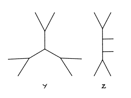
Figure 1: The two binary tree shapes on six leaves: (a) the shape $Y$; (b) the shape $Z$. There are 15 and 90 phylogenetic trees on a given leaf set that have the shapes $Y$ and $Z$, respectively.

We apply the above calculations to establish the following result.

Proposition 1

Let $T$ and $T^{\prime}$ be two unrooted binary phylogenetic trees of shapes $Z$ and $Y$ respectively. Consider a site pattern that is randomly generated on a coalescent tree on the same leaf set under the infinite alleles model with scaled mutation rate $\theta(=4N\mu)=\epsilon$. For a binary tree topology $W$, $\mathscr{P}_{W}(\chi)$ denote the parsimony score of a site pattern $\chi$ on $W$. Then

$$\mathbb{E}_{\mathrm{ESF}}[\mathscr{P}_{Z}(\chi)-\mathscr{P}_{Y}(\chi)]=\frac{1}{60}\epsilon+O(\epsilon^{2}).$$

where $\mathbb{E}_{\mathrm{ESF}}$ denotes the expectation under the infinite-alleles model.

Proof: We refer to a binary pattern on the leaf set $\{1,2,3,4,5,6\}$ as a $k$-clade if there are $k$ leaves in one state, and $6-k$ in another ($k\leq n/2$). Given such a binary pattern, the additional penalty of this clade is its homoplasy score (i.e. the parsimony score minus 1, unless the clade is a $0$-clade in which case the penalty is 0).

For a phylogenetic tree having shape $Y$ there are:

• $\binom{3}{2}\cdot 2\cdot 2=12$ in total 2-clades that cost an additional penalty of $+1$;

• $\frac{1}{2}\binom{3}{1}\cdot\binom{2}{1}\cdot 2=6$ in total 3-clades that cost an additional penalty of $+1$;

• $\frac{1}{2}2\cdot 2\cdot 2=4$ in total 3-clades that cost an additional penalty of $+2$.

Thus the expected value of the additional parsimony penalty $\Delta_{Y}$ for a tree phylogenetic tree having shape $Y$ is:

$$1\cdot P_{\epsilon,6}({\bf x})\cdot\frac{12}{\binom{6}{2}}+1\cdot P_{\epsilon,6}({\bf y})\cdot\frac{6}{\frac{1}{2}\binom{6}{3}}+2\cdot P_{\epsilon,6}({\bf y})\cdot\frac{4}{\frac{1}{2}\binom{6}{3}}.$$

Substituting Eqns. (1) and (2) into this last expression gives:

$$\mathbb{E}_{\mathrm{ESF}}[\mathscr{P}_{Y}(\chi)]=\frac{16}{15}\epsilon+O(\epsilon^{2}).$$ (3)

A similar analysis for a $Z$-shape tree shows that there are:

• $13$ in total 2-clades that cost an additional penalty of $+1$;

• $5$ in total 3-clades that cost an additional penalty of $+1$;

• $4$ in total 3-clades that cost an additional penalty of $+2$.

Thus the expected value of the additional parsimony penalty $\mathscr{P}_{Z}(\chi)$ for a tree phylogenetic tree having shape $Z$ is:

$$1\cdot P_{\epsilon,6}({\bf x})\cdot\frac{13}{\binom{6}{2}}+1\cdot P_{\epsilon,6}({\bf y})\cdot\frac{5}{\frac{1}{2}\binom{6}{3}}+2\cdot P_{\epsilon,6}({\bf y})\cdot\frac{4}{\frac{1}{2}\binom{6}{3}}.$$

Substituting Eqns. (1) and (2) into this last expression gives:

$$\mathbb{E}_{\mathrm{ESF}}[\mathscr{P}_{Z}(\chi)]=\frac{13}{12}\epsilon+O(\epsilon^{2}).$$ (4)

Combining Eqns. (3) and  (4) gives:

$$\mathbb{E}_{\mathrm{ESF}}[\mathscr{P}_{Z}(\chi)-\mathscr{P}_{Y}(\chi)]=\frac{1}{60}\epsilon+O(\epsilon^{2}).$$ (5)

Proposition 1 now follows from (5).

$\Box$

4 Proof of Theorem 1

Figure 2: Anomalous gene trees on a $6$-taxon species tree with shape $Z$. The event of deepest coalescence is depicted.

To establish Theorem 1 it suffices to do so for any number $n$ of taxa, and we do so for $n=6$. For the species tree $\mathcal{T}$, take any rooted tree that has the unrooted topology of the $Z$-shaped tree (caterpillar). Make all the edges $L$ of this tree less than $\beta$. We use the following notation:

• Denote by $G_{1},\ldots,G_{g}$ the gene trees generated by the multispecies coalescent on $\mathcal{T}$.

• Let $\mathbb{E}_{\mathcal{T}}$ denote the expectation under $\mathcal{T}$ and let $G$ be a gene tree generated under $\mathcal{T}$.

• Let $\mathcal{C}=[r]^{n}$ be the set of $r$-state characters on the set of $n$ taxa.

• Let $\chi_{k}^{f}\in\mathcal{C}$ be the $k$-th character of the $f$-th alignment, where $1\leq k\leq\ell$ and $1\leq f\leq g$, and let $\mathcal{X}=\{\chi_{k}^{f}\}_{k,f}$.

• For a character $\chi\in\mathcal{C}$, let $N_{\chi}^{f}$ be the number of times character $\chi$ appears in the $f$-th alignment and let $N_{\chi}$ be the number of times it appears overall.

Let $U$ be an $n$-leaf tree with mutation probabilites $\{q_{e}\}$. We denote by $p_{\chi}^{U}$ the probability that $\chi$ is produced by $U$ under the symmetric $r$-state site substitution model. Then the (mis-specified, i.e., not taking into account the coalescent) empirical minus log-likelihood under tree $U$ is given by

$$\mathscr{L}_{U}(\mathcal{X})=-\frac{1}{g\ell}\sum_{k,f}\log\left[rp_{\chi_{k}^{f}}^{U}\right]=-\frac{1}{g\ell}\sum_{\chi\in\mathcal{C}}N_{\chi}\log\left[rp_{\chi}^{U}\right].$$

We want to show that with high probability $\mathscr{L}_{U}(\mathcal{X})$ is not minimized on the species tree topology. We follow the proof sketched in Section 3.

For a binary tree topology $W$ and a character $\chi\in\mathcal{C}$ we let $\bar{\chi}^{W}$ denote a minimal extension of $\chi$ on $W$ and $\mathscr{P}_{W}(\chi)$, the parsimony score of $\chi$. Let

$$\mathscr{P}_{W}(\mathcal{X})=\frac{1}{g\ell}\sum_{k,f}\mathscr{P}_{W}(\chi_{k,f})=\frac{1}{g\ell}\sum_{\chi\in\mathcal{C}}N_{\chi}\mathscr{P}_{W}(\chi).$$

Let $E(W)$ and $V(W)$ be the edges and vertices of $W$. We assume that $W$ is binary and has $n$ leaves, hence $|E(W)|=2n-3$ and $|V(W)|=2n-2$. Let $\mathscr{L}_{W}^{*}(\mathcal{X})$ be the minus log-likelihood under an optimal choice of branch lengths (in $[0,+\infty]$) for $W$. Let $N_{0}$ denote the number of constant characters and $N_{\neq 0}=g\ell-N_{0}$.

Claim 1 (Parsimony-based approximation of the likelihood)

If

$$N_{0}>1,\qquad\frac{g\ell\mathscr{P}_{W}(\mathcal{X})}{N_{0}}\leq 1$$ (6)

then, for all $q_{0}\in(0,1)$,

$$\mathscr{L}_{W}^{*}(\mathcal{X})\leq-\mathscr{P}_{W}(\mathcal{X})\log\left(\frac{q_{0}}{r-1}\right)-2n\log\left(1-q_{0}\right)$$ (7)

and

$$\mathscr{L}_{W}^{*}(\mathcal{X})\geq-\mathscr{P}_{W}(\mathcal{X})\log\left(\frac{g\ell\mathscr{P}_{W}(\mathcal{X})}{(r-1)N_{0}}\right)-\frac{N_{\neq 0}}{g\ell}n\log r.$$ (8)

Proof: We adapt several bounds derived in Tuffley and Steel [30, Lemmas 5 and 6]. Letting $U$ have topology $W$ with all transition probabilities equal to $q_{0}$, by considering a minimal extension (see Tuffley and Steel [30, Equation (52)]) we have

$$rp_{\chi}^{U} \geq \left(\frac{q_{0}}{r-1}\right)^{\mathscr{P}_{W}(\chi)}\left(1-q_{0}\right)^{2n-3-\mathscr{P}_{W}(\chi)}$$

$$\geq \left(\frac{q_{0}}{r-1}\right)^{\mathscr{P}_{W}(\chi)}\left(1-q_{0}\right)^{2n},$$

and therefore

$$\mathscr{L}_{W}^{*}(\mathcal{X}) \leq -\frac{1}{g\ell}\left\{\sum_{\chi\neq 0}N_{\chi}\log\left[\left(\frac{q_{0}}{r-1}\right)^{\mathscr{P}_{W}(\chi)}\left(1-q_{0}\right)^{2n}\right]+N_{0}\log\left[\left(1-q_{0}\right)^{2n}\right]\right\}$$

$$= -\mathscr{P}_{W}(\mathcal{X})\log\left(\frac{q_{0}}{r-1}\right)-2n\log(1-q_{0}),$$

where we used that $N_{0}+\sum_{\chi\neq 0}N_{\chi}=g\ell$. This proves (7).

For the other direction, let $U$ be the tree with topology $W$ and optimal mutation probabilities $(q_{e}^{*})_{e}$. Let $\bar{q}=\max_{e}q_{e}$. Then, summing over all minimal extensions (see Tuffley and Steel [30, Equation (63)]),

$$rp_{\chi}^{U}\leq r^{n-2}\left(\frac{\bar{q}}{r-1}\right)^{\mathscr{P}_{W}(\chi)}\leq r^{n}\left(\frac{\bar{q}}{r-1}\right)^{\mathscr{P}_{W}(\chi)},$$

and by considering two leaves whose connecting path goes through an edge with probability $\bar{q}$ (see Tuffley and Steel [30, Equation (9)])

$$p_{0}^{U}\leq 1-\bar{q}.$$

Hence

$$\mathscr{L}_{U}(\chi) \geq -\frac{1}{g\ell}\left\{\sum_{\chi\neq 0}N_{\chi}\log\left[r^{n}\left(\frac{\bar{q}}{r-1}\right)^{\mathscr{P}_{W}(\chi)}\right]+N_{0}\log(1-\bar{q})\right\}$$

$$\geq -\frac{N_{\neq 0}}{g\ell}n\log r-\mathscr{P}_{W}(\mathcal{X})\log\left(\frac{\bar{q}}{r-1}\right)+\frac{N_{0}}{g\ell}\bar{q},$$

where we used $-\log(1-\bar{q})\geq\bar{q}$. Minimizing $\mathscr{L}_{U}(\chi)$ over $\bar{q}$ (see Tuffley and Steel [30, Equation (65) and (66)]), a lower bound is obtained by fixing $\bar{q}$ to $g\ell\mathscr{P}_{W}(\mathcal{X})/N_{0}$.

$\Box$

In order for the approximation in Claim 1 to be useful, we need that $N_{0}$ is asymptotically larger than $\max\{nN_{\neq 0},r\}$ and that $\mathscr{P}_{W}(\mathcal{X})$ is not too small. We proceed to prove that these two properties hold when the mutation rate is low enough.

We begin by showing that the empirical frequencies of characters are close to their expectation when $g\to+\infty$.

Claim 2 (Concentration of empirical frequencies)

With probability exceeding $1-2r^{n}\exp(-2g\zeta_{1}^{2})$, for all $\chi\in\mathcal{C}$,

$$\left|\frac{1}{g\ell}N_{\chi}-\mathbb{E}_{\mathcal{T}}[p_{\chi}^{G}]\right|<\zeta_{1}.$$ (9)

Proof: For all $\chi\in\mathcal{C}$,

$$\frac{1}{g\ell}N_{\chi}=\frac{1}{g\ell}\sum_{k,f}\mathbf{1}_{\{\chi_{k}^{f}=\chi\}}=\frac{1}{g}\sum_{f}\frac{1}{\ell}N_{\chi}^{f}=\frac{1}{g}\sum_{f}\left(\frac{1}{\ell}\sum_{k}\mathbf{1}_{\{\chi_{k}^{f}=\chi\}}\right).$$ (10)

Noting that the $\ell^{-1}N_{\chi}^{f}s$ are in $[0,1]$ and independent, Hoeffding’s inequality implies for all $\zeta>0$

$$\mathbb{P}_{\mathcal{T}}\left[\left|\frac{1}{g\ell}N_{\chi}-\frac{1}{g\ell}\mathbb{E}_{\mathcal{T}}[N_{\chi}]\right|\geq\zeta_{1}\right]\leq 2\exp\left(-2g\zeta_{1}^{2}\right).$$

Moreover by Eqn. (10)

$$\frac{1}{g\ell}\mathbb{E}_{\mathcal{T}}[N_{\chi}]=\frac{1}{g\ell}\sum_{k,f}\mathbb{E}_{\mathcal{T}}[\mathbf{1}_{\{\chi_{k}^{f}=\chi\}}]=\mathbb{P}_{\mathcal{T}}[\chi_{k}^{f}=\chi]=\mathbb{E}_{\mathcal{T}}[p_{\chi}^{G}].$$

The result follows from the fact that $|\mathcal{C}|=r^{n}$.

$\Box$

An immediate corollary is the concentration of the parsimony score.

Claim 3 (Concentration of parsimony score)

Under Eqn. (9),

$$\left|\mathscr{P}_{W}(\mathcal{X})-\mathbb{E}_{\mathcal{T}}[\mathscr{P}_{W}(\chi)]\right|\leq nr^{n}\zeta_{1}.$$

Proof: By definition,

$$\left|\mathscr{P}_{W}(\mathcal{X})-\mathbb{E}_{\mathcal{T}}[\mathscr{P}_{W}(\chi)]\right| = \left|\frac{1}{g\ell}\sum_{\chi}\mathscr{P}_{W}(\chi)N_{\chi}-\sum_{\chi}\mathscr{P}_{W}(\chi)\mathbb{E}_{\mathcal{T}}[p_{\chi}^{G}]\right|$$

$$\leq \sum_{\chi}\mathscr{P}_{W}(\chi)\left|\frac{1}{g\ell}N_{\chi}-\mathbb{E}_{\mathcal{T}}[p_{\chi}^{G}]\right|$$

$$\leq r^{n}n\zeta_{1}.$$

$\Box$

The next two claims relate the multispecies coalescent to the standard coalescent. We will refer to the population of $\mathcal{T}$ ancestral to all taxa as the master population. We let $\mathcal{D}$ be the gene tree event that no coalescence occurs before the master population, which we refer to as deepest coalescence. We let $\mathcal{T}_{\mathcal{D}}$ be the coalescent model on the master population (i.e., the standard $n$-coalescent). We further let $\mathcal{D}^{\prime}$ be the site event such that $\mathcal{D}$ occurs and further no mutation occurs below the master population. Let $M$ be the number of mutations on a site.

Claim 4 (Lower bound on the number of constant characters)

There is $\zeta_{2}$ (depending only on $n$ and $\beta$) such that, for any $\theta>0$,

$$\mathbb{E}_{\mathcal{T}}[p_{0}^{G}]\geq 1-\zeta_{2}\theta.$$

Proof: Note that

$$\{\chi=0\}\supseteq\{M=0\}.$$

The number of mutations on a site is stochastically dominated by the same quantity conditioned on $\mathcal{D}$. Indeed deepest coalescence ensures the highest total length of the gene tree. Hence

$$\mathbb{E}_{\mathcal{T}}[p_{0}^{G}]\geq\mathbb{P}_{\mathcal{T}}[M=0]\geq\mathbb{P}_{\mathcal{T}}[M=0\,|\,\mathcal{D}]=\mathbb{E}_{\mathcal{T}}\left[\exp\left(-\theta H_{G}\right)\,|\,\mathcal{D}\right]\geq\mathbb{E}_{\mathcal{T}}\left[1-\theta H_{G}\,|\,\mathcal{D}\right],$$

where $H_{G}$ is the total length of gene tree $G$. Note that, on $\mathcal{D}$,

$$H_{G}\leq n\cdot n\beta+H^{\prime}_{G},$$

where $H^{\prime}_{G}$ is the total length of the gene tree inside the master population. Letting $h^{(1)}_{n}$ be the expected length of the standard coalescent on $n$ samples, we have

$$\mathbb{E}_{\mathcal{T}}[p_{0}^{G}]\geq 1-\theta(n^{2}\beta+h^{(1)}_{n}).$$

Therefore we can take $\zeta_{2}=n^{2}\beta+h^{(1)}_{n}$.

$\Box$

Claim 5 (Reduction to standard coalescent)

For any $\theta$ and $\zeta_{3}>0$, there is $\beta$ small enough (depending only on $\zeta_{3}$, $n$, and $\theta$), such that

$$\left|\mathbb{E}_{\mathcal{T}}\left[\mathscr{P}_{W}(\chi)\right]-\mathbb{E}_{\mathcal{T}_{\mathcal{D}}}\left[\mathscr{P}_{W}(\chi)\right]\right|\leq\zeta_{3}.$$

Proof: Note that

$$\mathbb{E}_{\mathcal{T}}\left[\mathscr{P}_{W}(\chi)\,|\,\mathcal{D}^{\prime}\right]=\mathbb{E}_{\mathcal{T}_{\mathcal{D}}}\left[\mathscr{P}_{W}(\chi)\right].$$

Further

$$\mathbb{E}_{\mathcal{T}}\left[\mathscr{P}_{W}(\chi)\right] = \mathbb{E}_{\mathcal{T}}\left[\mathscr{P}_{W}(\chi)\,|\,\mathcal{D}^{\prime}\right]\mathbb{P}_{\mathcal{T}}[\mathcal{D}^{\prime}]+\mathbb{E}_{\mathcal{T}}\left[\mathscr{P}_{W}(\chi)\,|\,(\mathcal{D}^{\prime})^{c}\right]\mathbb{P}_{\mathcal{T}}[(\mathcal{D}^{\prime})^{c}]$$

$$\leq \mathbb{E}_{\mathcal{T}_{\mathcal{D}}}\left[\mathscr{P}_{W}(\chi)\right]+n\frac{\zeta_{3}}{n},$$

by choosing $\beta$ small enough to make the probability

$$\mathbb{P}_{\mathcal{T}}[\mathcal{D}^{\prime}]\geq(e^{-\binom{n}{2}\beta})^{n}\exp(-\theta(n\cdot n\beta))\geq 1-\frac{\zeta_{3}}{n}.$$

Above we used that $\mathscr{P}_{W}(\chi)\leq n$. Similarly,

$$\mathbb{E}_{\mathcal{T}}\left[\mathscr{P}_{W}(\chi)\right] = \mathbb{E}_{\mathcal{T}}\left[\mathscr{P}_{W}(\chi)\,|\,\mathcal{D}^{\prime}\right]\mathbb{P}_{\mathcal{T}}[\mathcal{D}^{\prime}]+\mathbb{E}_{\mathcal{T}}\left[\mathscr{P}_{W}(\chi)\,|\,(\mathcal{D}^{\prime})^{c}\right]\mathbb{P}_{\mathcal{T}}[(\mathcal{D}^{\prime})^{c}]$$

$$\geq \mathbb{E}_{\mathcal{T}_{\mathcal{D}}}\left[\mathscr{P}_{W}(\chi)\right]\left(1-\frac{\zeta_{3}}{n}\right)$$

$$\geq \mathbb{E}_{\mathcal{T}_{\mathcal{D}}}\left[\mathscr{P}_{W}(\chi)\right]-n\frac{\zeta_{3}}{n}.$$

$\Box$

Recall that $\mathbb{E}_{\mathrm{ESF}}$ is the expectation under the infinite-alleles model on $\mathcal{T}_{\mathcal{D}}$.

Claim 6 (Infinite-alleles approximation)

There is $\zeta_{4}$ depending only on $n$ such that, for any $\theta>0$,

$$\left|\mathbb{E}_{\mathcal{T}_{\mathcal{D}}}[\mathscr{P}_{W}(\chi)]-\mathbb{E}_{\mathrm{ESF}}[\mathscr{P}_{W}(\chi)]\right|\leq\zeta_{4}\theta^{2}.$$

Proof: Note that

$$\mathbb{E}_{\mathcal{T}_{\mathcal{D}}}[\mathscr{P}_{W}(\chi)\,|\,M\leq 1]=\mathbb{E}_{\mathrm{ESF}}[\mathscr{P}_{W}(\chi)\,|\,M\leq 1],$$

as a single mutation as the same effect on the characters of $r$-state symmetric and infinite-alleles models. Moreover, because both models are run with the same parameters, they have the same distribution of number of mutations. In particular,

$$\mathbb{P}_{\mathcal{T}_{\mathcal{D}}}[M\leq 1]=\mathbb{P}_{\mathrm{ESF}}[M\leq 1].$$

Note that

$$\mathbb{P}_{\mathrm{ESF}}[M>1] = \mathbb{E}_{\mathrm{ESF}}\left[\sum_{i\geq 2}e^{-\theta H_{G}}\frac{(\theta H_{G})^{i}}{i!}\right]$$

$$\leq \mathbb{E}_{\mathrm{ESF}}\left[(\theta H_{G})^{2}\sum_{i\geq 0}e^{-\theta H_{G}}\frac{(\theta H_{G})^{i}}{i!}\right]$$

$$= \theta^{2}h^{(2)}_{n},$$

where $h^{(2)}_{n}=\mathbb{E}_{\mathrm{ESF}}[H_{G}^{2}]$. Hence, since

$$\mathbb{E}_{\mathcal{T}_{\mathcal{D}}}[\mathscr{P}_{W}(\chi)] = \mathbb{E}_{\mathcal{T}_{\mathcal{D}}}[\mathscr{P}_{W}(\chi)\,|\,M\leq 1]\mathbb{P}_{\mathcal{T}_{\mathcal{D}}}[M\leq 1]$$

$$\qquad+\mathbb{E}_{\mathcal{T}_{\mathcal{D}}}[\mathscr{P}_{W}(\chi)\,|\,M>1]\mathbb{P}_{\mathcal{T}_{\mathcal{D}}}[M>1],$$

we have on the one hand

$$\mathbb{E}_{\mathcal{T}_{\mathcal{D}}}[\mathscr{P}_{W}(\chi)] \leq \mathbb{E}_{\mathrm{ESF}}[\mathscr{P}_{W}(\chi)\,|\,M\leq 1]\mathbb{P}_{\mathrm{ESF}}[M\leq 1]$$

$$\qquad+(\mathbb{E}_{\mathrm{ESF}}[\mathscr{P}_{W}(\chi)\,|\,M>1]+n)\mathbb{P}_{\mathrm{ESF}}[M>1]$$

$$= \mathbb{E}_{\mathrm{ESF}}[\mathscr{P}_{W}(\chi)]+n\theta^{2}h^{(2)}_{n}.$$

And, on the other hand, we have

$$\mathbb{E}_{\mathcal{T}_{\mathcal{D}}}[\mathscr{P}_{W}(\chi)] \geq \mathbb{E}_{\mathrm{ESF}}[\mathscr{P}_{W}(\chi)\,|\,M\leq 1]\mathbb{P}_{\mathrm{ESF}}[M\leq 1]$$

$$\qquad+(\mathbb{E}_{\mathrm{ESF}}[\mathscr{P}_{W}(\chi)\,|\,M>1]-n)\mathbb{P}_{\mathrm{ESF}}[M>1]$$

$$= \mathbb{E}_{\mathrm{ESF}}[\mathscr{P}_{W}(\chi)]-n\theta^{2}h^{(2)}_{n}.$$

$\Box$

Claim 7 (Final argument)

Let $\theta=\epsilon$. There are $\epsilon$ and $\beta$ small enough (depending on $n$ and $r$) such that $\mathscr{L}_{Z}^{*}(\mathcal{X})>\mathscr{L}_{Y}^{*}(\mathcal{X}),$ with probability exceeding $1-2r^{n}\exp(-2g\epsilon^{4})$.

Proof: Choosing $\beta$ small enough, $\zeta_{1}=\zeta_{3}=\epsilon^{2}.$ Claims 2 and 4 imply that, with probability exceeding $1-2r^{n}\exp(-2g\zeta_{1}^{2})$,

$$N_{0}\geq g\ell[1-\zeta_{2}\epsilon-\epsilon^{2}]=g\ell(1-O(\epsilon)),\qquad N_{\neq 0}=O(g\ell\epsilon).$$ (11)

When Eqn. (11) holds, by Claims 3,  5 and 6,

$$\left|\mathscr{P}_{W}(\mathcal{X})-\mathbb{E}_{\mathrm{ESF}}[\mathscr{P}_{W}(\chi)]\right|=O(\epsilon^{2}).$$ (12)

Together with Proposition 1, this implies that

$$\mathscr{P}_{Z}(\mathcal{X})-\mathscr{P}_{Y}(\mathcal{X})=\frac{1}{60}\epsilon+O(\epsilon^{2}).$$ (13)

We finally return to the likelihood. Note that (6) in Claim 1 is satisfied by (11) and

$$\mathscr{P}_{Y}(\mathcal{X})\leq nN_{\neq 0}/g\ell=O(n\varepsilon).$$ (14)

Hence, taking

$$q_{0}=g\ell\mathscr{P}_{Y}(\mathcal{X})/N_{0}=O(n\varepsilon),$$ (15)

in Claim 1 yields

$$\mathscr{L}_{Z}^{*}(\mathcal{X})-\mathscr{L}_{Y}^{*}(\mathcal{X}) \geq -[\mathscr{P}_{Z}(\mathcal{X})-\mathscr{P}_{Y}(\mathcal{X})]\log\left(\frac{g\ell\mathscr{P}_{Y}(\mathcal{X})}{(r-1)N_{0}}\right)$$

$$\qquad+2n\log\left(1-\frac{g\ell\mathscr{P}_{Y}(\mathcal{X})}{N_{0}}\right)-\frac{N_{\neq 0}}{g\ell}n\log r$$

$$\geq \left[\frac{1}{60}\epsilon+O(\epsilon^{2})\right]\log[\Omega((n\epsilon)^{-1})]$$

$$\qquad-2n\cdot O(n\epsilon)-n\log r\cdot O(\epsilon)$$

$$> 0,$$

by (14) and (15), when $\epsilon$ is small enough (depending on $n$ and $r$).

$\Box$

Theorem 1 now follows immediately from Claim 7 by noting that the lower bound $1-2r^{n}\exp(-2g\epsilon^{4})$ converges to 1 as $g$ grows; consequently, the probability that $Y$ has a higher likelihood than $Z$ (i.e. a lower minus log-likelihood) converges to $1$ as the number of alignments $g$ increases.

5 Concluding comments

Our statistical inconsistency result applies for the particular case of a tree with six leaves. While this suffices to establish inconsistency in general, we conjecture that an extension of our argument would apply to a tree with any number of leaves. However a detailed proof of this assertion is beyond the scope of this short note.

6 Acknowledgements

The authors thank the Simons Institute at UC Berkeley, where this work was carried out. S.R. is supported by NSF grants DMS-1248176 and DMS-1149312 (CAREER), and an Alfred P. Sloan Research Fellowship. M.S. would like to thank the NZ Marsden Fund and the Allan Wilson Centre for funding support.

References

- Bayzid and Warnow [2013] M. S. Bayzid and T. Warnow. Naive binning improves phylogenomic analyses. Bioinformatics, 29(18):2277–2284, 2013.
- Chifman and Kubatko [2014] J. Chifman and L. Kubatko. Identifiability of the unrooted species tree topology under the coalescent model with time-reversible substitution processes. arXiv, page 1406.4811, 2014.
- DeGiorgio and Degnan [2010] M. DeGiorgio and J. H. Degnan. Fast and consistent estimation of species trees using supermatrix rooted triples. Molecular Biology and Evolution, 27(3):552–569, 2010. doi: 10.1093/molbev/msp250. URL http://mbe.oxfordjournals.org/content/27/3/552.abstract.
- Degnan et al. [2009] J. Degnan, M. DeGiorgio, D. Bryant, and N. Rosenberg. Properties of consensus methods for inferring species trees from gene trees. Syst. Biol., 58(1):35–54, 2009.
- Degnan and Rosenberg [2009] J. H. Degnan and N. A. Rosenberg. Gene tree discordance, phylogenetic inference and the multispecies coalescent. Trends Ecol. Evol., 24(6):332–340, 2009.
- Durrett [2008] R. Durrett. Probability models for DNA sequence evolution (2nd ed.). Springer, 2008.
- Felsenstein [2004] J. Felsenstein. Inferring phylogenies, vol. 2. Sinauer Associates Sunderland, 2004.
- Gadagkar et al. [2005] S. R. Gadagkar, M. S. Rosenberg, and S. Kumar. Inferring species phylogenies from multiple genes: Concatenated sequence tree versus consensus gene tree. J. Exp. Zool. B Mol. Dev. Evol., 304:64–74, 2005.
- Gatesy and Springer [2013] J. Gatesy and M. S. Springer. Concatenation versus coalescence versus “concatalescence”. Proc. Natl. Acad. Sci. (USA)., 110(13):E1179, 2013.
- Heled and Drummond [2010] J. Heled and A. J. Drummond. Bayesian inference of species trees from multilocus data. Mol. Biol. Evol., 27(3):570–580, 2010.
- Huang et al. [2010] H. Huang, Q. He, L. S. Kubatko, and L. L. Knowles. Sources of error for species-tree estimation: Impact of mutational and coalescent effects on accuracy and implications for choosing among different methods. Syst. Biol., 59(5):573–583, 2010.
- Knowles and Kubatko [2010] L. L. Knowles and L. S. Kubatko. Estimating Species Trees: Practical and Theoretical Aspects. Wiley-Blackwell, 2010.
- Kubatko and Degnan [2007] L. S. Kubatko and J. H. Degnan. Inconsistency of phylogenetic estimates from concatenated data under coalescence. Syst. Biol., 56(1):17–24, 2007.
- Kubatko et al. [2009] L. S. Kubatko, B. C. Carstens, and L. L. Knowles. STEM: species tree estimation using maximum likelihood for gene trees under coalescence. Bioinformatics, 25(7):971–973, 2009. doi: 10.1093/bioinformatics/btp079. URL http://bioinformatics.oxfordjournals.org/content/25/7/971.abstract.
- Larget et al. [2010] B. R. Larget, S. K. Kotha, C. N. Dewey, and C. Ané. BUCKy: Gene tree/species tree reconciliation with Bayesian concordance analysis. Bioinformatics, 26(22):2910–2911, 2010. doi: 10.1093/bioinformatics/btq539. URL http://bioinformatics.oxfordjournals.org/content/26/22/2910.abstract.
- Leaché and Rannala [2011] A. D. Leaché and B. Rannala. The accuracy of species tree estimation under simulation: a comparison of methods. Syst. Biol., 60(2):126– 137, 2011.
- Liu et al. [2009a] L. Liu, L. Yu, L. Kubatko, D. K. Pearl, and S. V. Edwards. Coalescent methods for estimating phylogenetic trees. Molecular Phylogenetics and Evolution, 53(1):320– 328, 2009a.
- Liu et al. [2009b] L. Liu, L. Yu, D. K. Pearl, and S. V. Edwards. Estimating species phylogenies using coalescence times among sequences. Syst. Biol., 58(5):468– 477, 2009b.
- Maddison [1997] W. P. Maddison. Gene trees in species trees. Syst. Biol., 46(3):523–536, 1997.
- Meredith et al. [2011] R. W. Meredith, J. E. Janečka, J. Gatesy, O. A. Ryder, C. A. Fisher, E. C. Teeling, A. Goodbla, E. Eizirik, Simão. T. L. L., T. Stadler, D. L. Rabosky, R. L. Honeycutt, J. J. Flynn, C. M. Ingram, C. Steiner, T. L. Williams, T. J. Robinson, A. Burk-Herrick, M. Westerman, N. A. Ayoub, M. S. Springer, and W. J. Murphy. Impacts of the cretaceous terrestrial revolution and KPg extinction on mammal diversification. Science, 334(6055):521–524, 2011. doi: 10.1126/science.1211028. URL http://www.sciencemag.org/content/334/6055/521.abstract.
- Mirarab et al. [2014] Siavash Mirarab, Md Shamsuzzoha Bayzid, and Tandy Warnow. Evaluating summary methods for multi-locus species tree estimation in the presence of incomplete lineage sorting. Systematic Biology, 2014. doi: 10.1093/sysbio/syu063. URL http://sysbio.oxfordjournals.org/content/early/2014/08/26/sysbio.syu063.abstract.
- Mossel and Roch [2010] E. Mossel and S. Roch. Incomplete lineage sorting: consistent phylogeny estimation from multiple loci. IEEE/ACM Trans. Comput. Biol. Bioinf. (TCBB), 7(1):166 –171, 2010.
- Nichols [2001] R. Nichols. Gene trees and species trees are not the same. Trends Ecol. Evol., 16(7):358 –364, 2001.
- Roch [2013] S. Roch. An analytical comparison of multilocus methods under the multispecies coalescent: the three-taxon case. In Pacific Symposium on Biocomputing, pages 297– 306. World Scientific, 2013.
- Rokas et al. [2003] A. Rokas, B. L. Williams, N. King, and S. B. Carroll. Genome-scale approaches to resolving incongruence in molecular phylogenies. Nature, 425:798–804, 2003.
- Rosenberg [2002] N. A. Rosenberg. The probability of topological concordance of gene trees and species trees. Theor. Pop. Biol., 61:225– 247, 2002.
- Song et al. [2012] S. Song, L. Liu, S. V. Edwards, and S. Wu. Resolving conflict in eutherian mammal phylogeny using phylogenomics and the multispecies coalescent model. Proceedings of the National Academy of Sciences, 109(37):14942–14947, 2012.
- Steel [2013] M. Steel. Consistency of Bayesian inference of resolved phylogenetic trees. J. Theoret. Biol., 336:246–249, 2013.
- Tajima [1983] F. Tajima. Evolutionary relationships of DNA sequences in finite populations. Genetics, 105:437– 460, 1983.
- Tuffley and Steel [1997] C. Tuffley and M. A. Steel. Links between maximum likelihood and maximum parsimony under a simple model of site substitution. B. Math. Biol., 59(3):581–607, 1997.
- Wu et al. [2013] S. Wu, S. Song, L. Liu, and S. V. Edwards. Reply to Gatesy and Springer: The multispecies coalescent model can effectively handle recombination and gene tree heterogeneity. Proc. Natl. Acad. Sci. (USA), 110(13):E1180, 2013.