Quantifying Privacy: A Novel Entropy-Based Measure of Disclosure Risk

Abstract

It is well recognised that data mining and statistical analysis pose a serious treat to privacy. This is true for financial, medical, criminal and marketing research. Numerous techniques have been proposed to protect privacy, including restriction and data modification. Recently proposed privacy models such as differential privacy and k-anonymity received a lot of attention and for the latter there are now several improvements of the original scheme, each removing some security shortcomings of the previous one. However, the challenge lies in evaluating and comparing privacy provided by various techniques. In this paper we propose a novel entropy based security measure that can be applied to any generalisation, restriction or data modification technique. We use our measure to empirically evaluate and compare a few popular methods, namely query restriction, sampling and noise addition.

1 Introduction

Proliferation of computer, network and communication technology and applications, and in particular social networking and cloud computing had a great impact on the way personal data is collected, stored and used. Data collected in one location (e.g., hospital) can now be stored remotely in a cloud and accessed from anywhere in the world. These advances have undoubtedly changed the way we think about privacy [28, 4, 18] and what once could have been regulated by legislative measures alone now requires a sophisticated suite of privacy enhancing technologies. In this study we are concerned with a situation where confidential personal data is made available to a wide range of users who are authorised to perform data mining and statistical analysis, but not to access any individual data. There are various Statistical Disclosure Control (SDC) techniques that can be used to alleviate this problem [40, 2, 5, 13, 20] but, unfortunately, none of them is able to solve it completely, due to its intrinsic contradictory nature. On one hand, one must keep the risk of individual value disclosure as low as possible. On the other hand, the utility (usefulness) of the data must remain high. However, low risk implies low utility and high utility implies high risk. A good SDC technique aims at finding a right balance between the two. In order to achieve this balance, it is crucial to adequately measure both utility and disclosure risk. While measuring data utility has been well studied in the literature  [7, 9, 10, 11, 12, 22, 40], measuring disclosure risk is still considered as a difficult problem and has been only partly solved.

Contribution: (1) In this paper we propose a novel entropy based measure of disclosure risk, which we refer to Confidential Attribute Equivocation (CAE), and which is independent of the underlying SDC technique, and thus can always be used. The main novelty and advantage of our technique over similar ones is that it takes into account the candidate confidential values themselves, rather than just their probabilities, and is thus able to capture the risk of approximate disclosure of confidential values, rather than the exact disclosure alone. (2) We develop an efficient dynamic programming algorithm to evaluate the CAE. (3) We show how our technique can be applied to evaluate a few common SDC techniques, including sampling, query restriction and noise addition.

This paper is organised as follows. In the next section we present related work on disclosure risk measures and in Section 3 we present a scenario that is not adequately covered by any of the previous measures and introduce a novel entropy-based measure. In Section 4 we present a dynamic programming algorithm for calculating the disclosure risk, in Section 5 we use our measure to empirically evaluate a few existing SDC techniques, and in Section 6 we discuss the experimental results and give some concluding remarks.

2 Introduction to Statistical Disclosure Control and Related Work on Disclosure Risk Measures

Privacy is an elusive concept, and many privacy models have been proposed, with varying success. We next present a few of the most prominent models, including $k$-anonymity and differential privacy.

In a data set, some attributes may be considered public knowledge and used to identify records. They are refereed to as “identifying” attributes or “quasi-identifiers” (QI). A class of records where values of all QI attributes are the same is called equivalence class. To limit disclosure, Samarati and Sweeney [32] proposed a so-called k-anonymity that requires each equivalence class to have no less than $k$ records. The main problem with k-anonymity arises when all the records in an equivalence class share the same confidential value, which allows intruder to disclose the confidential value without actually re-identifying the record. In order to alleviate this problem, Machanavajjhala et al proposed l-diversity [30], which in its simplest form requires every QI to contain at least $l$ distinct values. While this model is indeed a great improvement over $k$-anonymity, it does not consider how close these values are from each other, and thus leaves room for approximate disclosure of confidential values. Li et al. [29] introduced t-closeness, which considers the distribution of confidential attribute values in each equivalence class and the distribution of the confidential attribute values in the whole dataset, and requires that the distance between these two distributions does not exceed a given threshold t. While it greatly reduces the disclosure risk, t-closeness is overly restrictive and severely impacts the utility of data. In this context, our measure of disclosure risk can be seen as bridging a gap between the l-diversity and the rigid t-closeness.

Another prominent privacy model is differential privacy [16], which requires that the results to all queries allowed on the database do not change significantly if a single record is added or deleted from the database. While this is certainly an efficient model against table linkage attack, it is not design to prevent attribute and record linkage [20] and in practice may be inferior to k-anonymity [36].

Each one of the above models can be implemented using different SDC techniques, which can be classified as modification techniques and query restriction techniques [13, 5, 40, 14]. Modification techniques involve some kind of alternation of the original data set before it is released to statistical users. This includes noise addition, data swapping, aggregation, suppression and sampling [5, 13, 23, 8, 24]. The common denominator of all modification techniques is that the modified dataset is released to users who are free to perform any query on it, but the answers they get are only approximate and not exact. On the other hand, query restriction techniques do not release database to a user but rather provide a query access. The SDC system decides whether or not to answer the query but if the query is answered, the answer will always be exact and not approximate as with modification techniques [14, 5].

In this study we are not concerned with SDC techniques or privacy models as such but rather with measuring disclosure risk. In the literature, disclosure risk measures are classified as measures for record re-identification or confidential value disclosure [15, 27, 5]. The latter focuses on measuring the risk of compromising a confidential value of a particular individual, while the former focuses on measuring the risk of inferring an individual’s identity. In either case the disclosure risk measures may be applied to the database as a whole, or to individual records.

Several methods have been proposed to estimate the disclosure risk in sampling and they fall under the category of record identification. Winkler [41] refers to these methods as Sample-Unique-Population-Unique (SUPU) methods as disclosure risk estimation requires assessing the uniqueness of records in the released sample and in the population. Skinner and Eliot [34] introduced a new disclosure risk measure for microdata which falls under SUPU methods [41]. Their measure is based on the probability $\theta=Pr(\mbox{correct match}|\mbox{unique match})$ that a microdata record and a population unit are correctly matched. Additionally, they introduced a simple variance estimator and claimed that their measure is able to evaluate the different ways of releasing microdata from a sample survey. Truta et el. [39] introduced other SUPU measures and termed them minimal, maximal, and weighted disclosure risk measures. The minimal disclosure risk measure is the percentage of records in a population that can be correctly re-identified by an intruder. All these records must be population unique. The maximum disclosure risk measure takes into account records that are not population unique while the weighted disclosure risk measure assigns more weights to unique records over other records. Their measures are not linked to a certain individual but compute the overall disclosure risk for the database. These measures can only be applied to limited SDC methods such as sampling and microaggregation and it is considered hard to choose the disclosure risk weight matrix [39]. However, assigning weights enables a data owner to setup different levels of confidentiality. These measures are useful in deciding the order of applying more than one SDC method on the initial data.

Trottini and Fienberg [38] proposed a simple Bayesian model for capturing user uncertainty after releasing the data by an agency. They distinguish between the legitimate user (researcher) uncertainty and the malicious user (intruder) uncertainty. This distinction is used as the basis of defining appropriate disclosure risk measure. The proposed measure is an arbitrary decreasing function of the user’s uncertainty about a confidential attribute value.

Spruill [35] measured confidentiality as a percentage of records in the released data where a link with the original data can not be made. In order to decide if there is such a link, for each released record, we add up either the square or the absolute value of the difference between the released value and the true value for all common numerical attributes. A link is said to be made if a released record was derived from the true record that has the minimum sum of differences. Spruill’s early work gave rise to record linkage, much studied in recent years [20].

There are some recent proposals that use information-theoretic approach to measure privacy and utility of various SDC techniques [31, 33]; however, none of them measures the “approximate” compromise, as we explain in the next section.

3 A Novel Entropy-Based Measure

Out of all disclosure risk measures, the closest to our proposal is a measure proposed by Onganian and Domingo-Ferrer [31] that evaluates the security of releasing tabular data. The measure is equal to the reciprocal of conditional entropy given the knowledge of an intruder:

$$DR(X)=\frac{1}{H(X|Y=y)}=\frac{1}{(-\sum_{x}p(x|y)\log_{2}p(x|y))}$$ (1)

where X represents a confidential attribute for a given record and Y represents intruder’s knowledge. The disclosure risk is inversely proportional to the uncertainty about the confidential attribute given intruder’s knowledge. The measure performs a posteriori, that is, after applying one of SDC methods to the tables. It is a complement to a priori measures such as some currently used sensitivity rules including (n,k)-dominance and pq-rule, which help a data owner in deciding whether to release the data or not. The main strength of the above a posteriori measure is its generality: it is applicable to various SDC methods such as Cell Suppression, Rounding, and Table Redesign. In order to evaluate this disclosure risk, one has to find a set of the possible confidential attribute values and their probabilities given the condition $Y=y$. A down side of this measure is that it does not capture accurately the knowledge that an intruder has about a confidential attribute, as it does not give careful consideration to the attribute values but only the probabilities with which the values occur. Our proposed method considers the attribute values in addition to their probabilities.

Before we proceed to describe our measure in more detail and compare some of the SDC techniques in the experimental section, we need to introduce the concept of “database compromise”. We say that a database is compromised if a sensitive statistic is disclosed  [14]. There are several distinct types of compromise, depending upon what is considered to be sensitive. For example, if only exact individual values are considered sensitive, we have the so-called exact compromise. Approximate compromise occurs when a user is able to infer that a confidential individual value $X$ lies within a range $[X_{0}-\frac{\huge{\varepsilon}}{2},X_{0}+\frac{\huge{\varepsilon}}{2}]$ for some predefined value of $\huge{\varepsilon}$. Approximate compromise will prove crucial for the definition of our new security measure.

We consider a scenario where an intruder is trying to unlawfully disclose confidential information from a database. She uses all the available information she can get from the database, as well as any external knowledge she may have. At the end of her analysis, the intruder is able to reduce the possibilities and limit her suspicion to certain data values. Shannon’s entropy can measure the intruder’s uncertainty, but does not take into consideration how far or close these values are from each other.

Table 1: Two Examples

	Example 1	Example 2
Q1:	SELECT MAX(Salary)	SELECT MAX(Salary)
	FROM AcademicStaff	FROM AcademicStaff
	WHERE Sex = ”F”	WHERE Age = $37$
A1:	Maximum salary = $107,000$	Maximum salary = $80,000$
Q2:	SELECT AVG(Salary)	SELECT AVG(Salary)
	FROM AcademicStaff	FROM AcademicStaff
	WHERE Sex = ”F”	WHERE Age = $37$
A2:	Average salary = $78,500$	Average salary = $78,500$

The first example in Table 1  shows the queries submitted by the intruder and the database response to them. Assuming that there are only two female academics, Layla and Angela, the intruder learns that Layla’s salary is one of the two values: It is either $107K$ or $50K$.

In the second example we assume that there are only two academics aged $37$, Qays and Tony. Then the intruder knows that Qays’s salary is either $80K$ or $77K$. If we use Shannon’s entropy to evaluate the intruder’s uncertainty in examples $1$ and $2$, we get the same result, 1 bit in each case. However, we argue that the intruder learns more in example $2$, as he can pretty accurately estimate the salary to be $78.5K\pm 1.5K$. This highlights the need for more accurate measure than Shannon’s entropy, which would be able to capture such differences.

Recall that a compromise can be exact or approximate. Shannon’s entropy can be considered a satisfactory measure for the disclosure risk that is related to the exact compromise. However, in the approximate compromise, we argue that Shannon’s entropy does not express precisely the intruder’s knowledge about a particular confidential value.

We introduce a notion of privacy for the so-called approximate compromise range ($\huge{\varepsilon}$). In the approximate compromise an intruder learns that the confidential value $X$ lies within a range $[X_{0}-\frac{\huge{\varepsilon}}{2},X_{0}+\frac{\huge{\varepsilon}}{2}]$. For the two example we have $X\in[X_{0}-28.5K,~{}X_{0}+28.5K]$ for Layla and $X\in[X_{0}-1.5K,~{}X_{0}+1.5K]$ for Qay, where in both cases $X_{0}=78.5K$. Obviously, the intruder knows more about Qay’s than Layla’s salary, as in the former the approximate compromise range is $3K$, while in the latter it is $57K$.

To capture the information about the range $\huge{\varepsilon}$, we use Shannon’s entropy $H$ as a function of $\huge{\varepsilon}$. The graphs in Figure 1 correspond to the intruder’s uncertainty $H(\huge{\varepsilon})$ in the above examples. We notice that the entropy $H(0)$ is the same in both cases, that is, the disclosure risks are the same for exact compromise. However, the area under $H(\huge{\varepsilon})$ is much larger for Layla implying that this case is more resistant against approximate compromise.

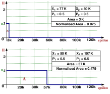
Figure 1: Our Security Measure: for (77K, 80K) and (50K, 107K).

In general, we can then evaluate intruder’s uncertainty for any given $\huge{\varepsilon}$. In particular, we use $H_{0}=H(0)$ to denote intruder’s uncertainty in the case of exact compromise, that is, approximate compromise range of “$0$” and we call it initial entropy. Additionally, in what follows we examine the area ($A$) determined as an integral: $A=\int_{0}^{\huge{\varepsilon}_{max}}H(\huge{\varepsilon})$, where “$\huge{\varepsilon}_{max}$” is the value of $\huge{\varepsilon}$ for which entropy $H(\huge{\varepsilon})$ drops to zero. Formally, $H(\huge{\varepsilon}_{max}=0)$ and $H(\huge{\varepsilon}>0)$ for all $\huge{\varepsilon}<\huge{\varepsilon}_{max}$

We next explain how $H(\huge{\varepsilon})$ is calculated in general. We introduce a “window” of length $\huge{\varepsilon}$. When a window “covers” two or more values, then they are replaced with a single value whose probability is equal to the sum of probabilities of all the values covered by the window. In general, there will be more than one way to cover the values with windows of length $\huge{\varepsilon}$ and we need to select the way that minimises the entropy $H(\huge{\varepsilon})$. We next formally define the problem of calculating $H(\huge{\varepsilon})$.

Calculating $H(\huge{\varepsilon})$
Input:
* Sorted values $x_{1},x_{2},\dots,x_{n}$, $x_{i}>x_{j}$ for any $i>j$
* Their corresponding probabilities: $p_{1},p_{2},\dots,p_{n}$
* Parameter $\huge{\varepsilon}\leq x_{n}-x_{1}$
Output:
* Collection $C$ of subsets $(x_{1},...x_{y_{1}}),(x_{y_{1}+1},...,x_{y_{2}}),\dots,(x_{y_{m}+1},...,x_{n})$, such that (1) $x_{y_{1}}-x_{1}\leq\huge{\varepsilon}$, (2) $x_{y_{i}}-x_{y_{i-1}+1}\leq\huge{\varepsilon}$, $2\leq i\leq m$, (3) $x_{n}-x_{y_{m}+1}\leq\huge{\varepsilon}$
* Corresponding probabilities $q_{1}=p_{1}+...+p_{y_{1}},...,q_{m+1}=p_{y_{m}+1}+...+p_{n}$
* $H(\huge{\varepsilon})$ calculated over probabilities $q$, such that $H(\huge{\varepsilon})$ is maximised over all collections $C$ satisfying conditions above.

Computing the minimum entropy $H(\huge{\varepsilon})$ as a function of $\huge{\varepsilon}$ is not straightforward and in Appendix we provide an example to illustrate the entropy calculation. In the next section we introduce a dynamic programming algorithm to find the optimal entropy and hence calculate the area ($A$) that together with the initial entropy ($H_{0}$) represents our disclosure risk.

4 A Dynamic Programming Algorithm to Compute $H(\huge{\varepsilon})$

We are given as input a set of values $x_{i}$ in increasing order ($x_{1}<x_{2}<x_{3}<\cdots<x_{n}$) where each $x_{i}$ has a given probability $p_{i}$ where $p_{i}~{}\geq~{}0$ and and $\Sigma p_{i}=1$. In order to produce our security measure, we need to calculate minimum $H(\huge{\varepsilon})$ for each $\huge{\varepsilon}$. We break the problem into stages (rows) and states (columns). Each row in the table corresponds to a stage or $\huge{\varepsilon}$. Column “$i$” in the table corresponds to the subproblem containing values $x_{1},~{}x_{2},\cdots,~{}x_{i}$. For a given row (stage) in the table, each cell in this row is viewed as a subproblem  $H(\huge{\varepsilon},i)$ of the original problem $H(\huge{\varepsilon})$. For a given stage and state,  $H(\huge{\varepsilon},i)$  is computed by the following recurrence:

$$H(\huge{\varepsilon},i)=min[(H(\huge{\varepsilon},i-1)+a_{i}),(H(\huge{\varepsilon},i-2)+a_{i-1}),...,(H(\huge{\varepsilon},j-1)+a_{j})]$$

where

$$a_{j}=(\sum_{k=j}^{i}p_{k})\cdot log(\frac{1}{(\sum_{k=j}^{i}p_{k})})$$

$X_{i}-X_{j}\leq\huge{\varepsilon}$, $X_{i}-X_{j-1}>\huge{\varepsilon}$ for $i,j\in[1,n]$ and $i\geq j$

$$H(0,\huge{\varepsilon})=0$$

$$H(1,\huge{\varepsilon})=p_{1}\cdot log(\frac{1}{p_{1}})$$

Input: $x[~{}]$: a set of integer values in ascending order;

           $p[~{}]$: a set of probabilities corresponding to the above integer values.

Output: $H(\huge{\varepsilon})$

$H_{0}\leftarrow\sum_{i=1}^{n}p(x_{i})\cdot log(\frac{1}{p(x_{i})})$;

foreach $\huge{\varepsilon}$ do  $H(\huge{\varepsilon},0)\leftarrow 0$;

$H(\huge{\varepsilon},1)\leftarrow p_{1}\cdot\log(\frac{1}{p_{1}})$;

for $i\leftarrow 2$ to $n$ do  $j\leftarrow i$;

$p_{partial}\leftarrow 0$;

$H(\huge{\varepsilon},i)\leftarrow H(\huge{\varepsilon-1},i)$;

while $(x_{i}-x_{j}\leq\huge{\varepsilon})~{}and~{}(j\neq 0)$ do  $p_{partial}\leftarrow p_{partial}+p_{j}$;

$H_{temp}\leftarrow p_{partial}\cdot\log(\frac{1}{p_{partial}})+H(\huge{\varepsilon},j-1)$;

if $H_{temp}<H(\huge{\varepsilon},i)$ then  $H(\huge{\varepsilon},i)\leftarrow H_{temp}$;

end $j\leftarrow j-1$;

end end $H(\huge{\varepsilon})\leftarrow H(\huge{\varepsilon},n)$;

Display: $H(\huge{\varepsilon})$ end

Algorithm 1 A dynamic programming algorithm to compute $H(\huge{\varepsilon})$

5 The Experiments: Description and Implementation

In this section we apply our proposed security measure to a few common Statistical Disclosure Control (SDC) techniques. In all instances we assume that the intruder has supplementary knowledge (SK) about an individual whose corresponding record is stored in the original dataset, which can be as limited as one attribute or can be as extensive as all attributes except the confidential one.

The comparative study is performed on three different data sets. Here we present results on PUMS dataset, whose decription can be found in the Appendix.

Sampling. In this experiment, we release a subset of records (sample) from the original microdata file (population). We use a simple random sample without replacement where each record in the original is equally likely to be included in the produced sample and duplicates are not allowed. The produced sample has a constant size specified as a percentage of the original dataset total size and referred to as “sampling size” (or “sampling factor”). In deciding on the structure of the sampling experiment, we follow work by Truta et el. [39] on disclosure risk measures for sampling, where we compute the overall disclosure risk for the database, rather than for a certain individual.

In order to study the effect of sample size on the security we use four different sampling factors: $5\%,10\%,20\%,50\%$. For each sample size, we generate $30$ different sample files. Additionally, we study the effect of the intruder’s supplementary knowledge. We start with supplementary knowledge as little as one attribute and extended it to reach all attributes except the confidential one. For each attribute we performed experiments for all possible values. The results in Figure 2 are the averaged over all 30 samples, all attributes and all values.

Query Restriction. In this experiment, we consider a scenario where an intruder submits a set of range queries to a DBMS. The intruder performs an analysis using the answers to the submitted queries as well as the supplementary knowledge with an aim to infer a confidential attribute value for the given record, e.g salary in PUMS dataset. We assume that the intruder has build a system of linear equations out of the responses to range queries. We use $Q=2l$ to denote the query set size for the queries a user (i.e., an intruder) is permitted to ask. For simplicity, we only consider even query set sizes. We use $k$ to denote the number of queries and thus also the number of linear equations: $k=\lfloor\frac{2n}{Q}\rfloor-1$.

We run the experiment for $5$ different query set size $\{2,4,8,16,32\}$. For each query set size, we shuffle the records in the original dataset to get different systems of linear equations. For each query set size, we produce randomly $30$ different systems of linear equations. Just like in the case of sampling, for each attribute we performed experiments for all possible values. The results in Figure 2 are the average results, over all $30$ systems of linear equations, all SK attributes and all values.

Noise Addition. We consider a scenario where a DBMS alters an original dataset by adding certain level of noise. The noise is added to all attributes in the dataset, sensitive and non-sensitive, categorical and numerical. We use additive noise studied in [25, 37, 19, 26, 43]. The amount of noise is drawn randomly from binomial probability distribution as the nature of attributes in our dataset is discrete. The DBMS then releases the perturbed version of the dataset and an intruder obtains a copy of it. The intruder performs an analysis using the released perturbed dataset together with the supplementary knowledge with an aim to infer a confidential attribute value, e.g salary in PUMS dataset, corresponding to the individual of concern. We assume there is only one confidential attribute; it is straightforward to generalize our experiments to cover more than one confidential attribute.

6 Discussion and Conclusion

As expected, for all three SDC techniques our privacy measure, CAE, increases with decrease in utility (Figure 2). In Sampling, utility is proportional to the sample size, in Query Restriction utility is inversely proportional to the query size, and in Noise Addition utility is inversely proportional to the amount of noise.

The experiments also show that privacy declines with additional supplementary knowledge that intruder might have, which is expressed on horizontal axis as the number of known attributes. We note that this decline is sometimes gentle and sometimes sharp, depending on the utility which is in Figure 2 given as a parameter: for low utility privacy only gently declines with supplementary knowledge, while for higher utility the decline is typically sharp.

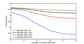
(a) Sampling: $H_{0}$ vs SK

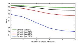
(b) Sampling: Area vs SK

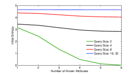
(c) QueryRestr.: $H_{0}$ vs SK

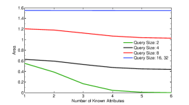
(d) QueryRestr.:Area vs SK

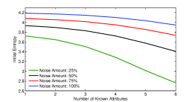
(e) NoiseAdd.: $H_{0}$ vs SK

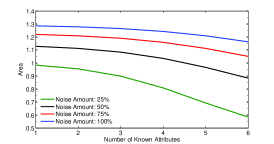
(f) NoiseAdd.: Area vs SK

Figure 2: Sampling, Query Restriction and Noise Addition

Importantly, our experiments demonstrate how we can compare different SDC techniques and select the most suitable one for specific application and requirements. For example, in the absence of supplementary knowledge sampling with size 50% and query restriction with query set size 8 provide similar level of privacy (blue line in Figure (a) and red line in Figure (c)); however, the privacy sharply drops with supplementary knowledge increases in sampling, while it remains flat in query restriction. Moreover, Figures (b) and (d) that indicate approximate compromise show a slight superiority of sampling in the absence of supplementary knowledge, but as supplementary knowledge grows sampling becomes much more vulnerable than query restriction.

In summary, unlike previously proposed privacy measures, our novel information theoretic privacy measure (CAE) has the ability to capture approximate compromise; it can also be applied to any SDC technique, as long as the probabilities of different confidential values can be estimated. In this paper we considered the most common SDC techniques and showed how CAE can be used to evaluate the privacy they offer, and how this privacy relates to both utility and supplementary knowledge.

Appendix

Calculation entropy

We demonstrate on a small example how $H(\huge{\varepsilon})$ is calculated. Consider as input a set of values $x_{i}$ of a confidential attribute $X$, where for each $x_{i}$ we have a given probability $p_{i}$, where $p_{i}~{}\geq~{}0$ and $\Sigma p_{i}=1$. In order to produce our security measure and compute the area, we need to calculate $H(\huge{\varepsilon})$ for each $\huge{\varepsilon}$. In our example, an intruder learns that a confidential variable $X~{}\in~{}[1-10]$ has four possible values with probabilities as follow:

$x_{1}~{}=~{}1$	$x_{2}~{}=~{}3$	$x_{3}~{}=~{}8$	$x_{4}~{}=~{}9$
$p_{1}~{}=~{}0.15$	$p_{2}~{}=~{}0.1$	$p_{3}~{}=~{}0.7$	$p_{4}~{}=~{}0.05$

1. We start by calculating initial entropy $H(\huge{\varepsilon}=0)$, as the approximate compromise range $\huge{\varepsilon}$ is initially “$0$”; this is equivalent to Shannon’s entropy for given events and their probabilities:

   $$H(0)=\sum_{i=1}^{4}p(x_{i})\cdot log(\frac{1}{p(x_{i})})=1.319$$

   

2. We calculate the minimum entropy when $\huge{\varepsilon}=1$, that is, $H(\huge{\varepsilon}=1)$. We cover $x_{3}$ and $x_{4}$ with window of length $1$ and we obtain a combined value $x_{3,4}=8.5$ with probability $p_{3,4}=p_{3}+p_{4}=0.75$:

   $$H(1)=p{1}\cdot log(\frac{1}{p{1}})~{}+~{}p{2}\cdot log(\frac{1}{p{2}})~{}+~{}(p{3}+~{}p{4})\cdot log(\frac{1}{(p{3}+~{}p{4})})=1.054$$

   

3. We calculate the minimum entropy when $\huge{\varepsilon}=2$, that is, $H(\huge{\varepsilon}=2)$. We cover $x_{3}$ and $x_{4}$ with window of length $1$ and $x_{1}$ and $x_{2}$ with window of length $2$:

   $$H(2)=H(X)=(p{1}+~{}p{2})\cdot log(\frac{1}{(p{1}+~{}p{2})})~{}+~{}(p{3}+~{}p{4})\cdot log(\frac{1}{(p{3}+~{}p{4})})=0.811$$

   

4. When $\huge{\varepsilon}=3$ or $4$, we can not do better than for $\huge{\varepsilon}=2$.

5. We calculate the minimum entropy when $\huge{\varepsilon}=5$, that is, $H(\huge{\varepsilon}=5)$. Here we have $2$ options so as how to cover the values with window of length $5$ or less. We choose with the option that gives us the minimum entropy, that is, covering $x_{3}$ and $x_{4}$ with window of length $1$ and $x_{1}$ and $x_{2}$ with window of length $2$:

   $$H(5)=H(X)=p{1}\cdot log(\frac{1}{p{1}})~{}+(p{2}+~{}p{3})\cdot log(\frac{1}{(p{2}+~{}p{3})})~{}+~{}p{4}\cdot log(\frac{1}{p{4}})=0.884$$

   

   $$H(5)=H(X)=(p{1}+~{}p{2})\cdot log(\frac{1}{(p{1}+~{}p{2})})~{}+~{}(p{3}+~{}p{4})\cdot log(\frac{1}{(p{3}+~{}p{4})})=0.811$$

6. We calculate the minimum entropy when $\huge{\varepsilon}=6$, that is, $H(\huge{\varepsilon}=6)$. We cover $x_{2},x_{3}$ and $x_{4}$ with window of length $6$:

   $$H(6)=p{1}\cdot log(\frac{1}{p{1}})~{}+(p{2}+~{}p{3}+~{}p{4})\cdot log(\frac{1}{(p{2}+~{}p{3}+~{}p{4})})=0.61$$

   

7. We calculate the minimum entropy when $\huge{\varepsilon}=7$, $H(\huge{\varepsilon}=7)$. We cover $x_{1},x_{2}$ and $x_{3}$ with window of length $7$:

   $$H(7)=(p{1}+~{}p{2}+~{}p{3})\cdot log(\frac{1}{(p{1}+~{}p{2}+~{}p{3})})~{}+~{}p{4}\cdot log(\frac{1}{p{4}})=0.286$$

   

8. We calculate the minimum entropy when $\huge{\varepsilon}=8$, $H(\huge{\varepsilon}=8)$. The window of length $8$ is wide enough to cover all the values and thus will produce an entropy of zero:

   $$H(8)=(p{1}+~{}p{2}+~{}p{3}+~{}p{4})\cdot log(\frac{1}{(p{1}+~{}p{2}+~{}p{3}+~{}p{4})})=0$$

   

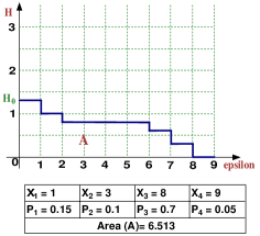
Figure 3: Our security measure for the numerical example.

Figure 3 shows $H(\huge{\varepsilon})$ and the computed area ($A$) for the above example. This calculation illustrates that computing the minimum entropy $H$ as a function of $\huge{\varepsilon}$ is not a straightforward task, as we have to make choices. In order to solve this problem efficiently, we design a dynamic programming algorithm to find the optimal entropy for each $\huge{\varepsilon}$ as a measure of disclosure risk (see Section 4).

PUMS Dataset

Our first data set is the Public Use Microdata Sample (PUMS) [1] (experiments on other datasets are ommitted due to length restriction of the paper). It is a sample of the actual responses to the American Community Survey (ACS) and is offered by the U.S. Census Bureau. We have chosen Illinoi state sample for the year $2006$ as a dataset. The dataset consists of $2500$ records. Each record is described by $7$ selected attributes that are shown in Table 2. The first column in the table shows the selected attributes. The minimum and maximum value for each attribute are shown in the second and third columns. For example, the minimum value for “$Salary$” is $10$ while the maximum is $250$. The fourth column indicates the data type for the corresponding attribute and it can be one of the following: Categorical, Numerical-Integer, or Numerical-Real. The next column, Rounding, indicates if the corresponding attribute values have been rounded. For example, for the attribute “$Salary$”, we round values to the nearest $10~{}K$. Symbol ”-” indicates no rounding. The last column contains number of values in the actual domain for the corresponding attribute after rounding. We select the first attribute, “$Salary$”, to be sensitive (confidential) and hence we need to keep its value confidential.

Table 2: The selected attributes from PUMS dataset

Attribute	Min.	Max.	Data Type	Rounding	No of Values
Salary	$10$	$250$	$Numerical-Integer$	$10$	$25$
Age	$16$	$84$	$Numerical-Integer$	$-$	$69$
Sex	$1$	$2$	$Categorical$	$-$	$2$
Education	$1$	$16$	$Categorical$	$-$	$16$
Industry	$1$	$18$	$Categorical$	$-$	$18$
Occupation	$1$	$25$	$Categorical$	$-$	$25$
Work Travel Time	$1$	$177$	$Numerical-Integer$	$-$	$177$

Details of Experiments

We use the following notation: (1) $n$ is a number of records in the original database; (2) $C$ is the confidential attribute; (3) $c_{i}$, $1\leq i\leq n$, is the value of the confidential attribute $C$ in record $i$; (4) $D$ is the domain of the confidential attribute $C$ in the original database; (5) $d_{i}$ is the $i^{th}$ value of the confidential attribute in the domain $D$, where $1\leq i\leq|D|$; (6) $p_{i}$ is the probability that the confidential attribute value is $d_{i}$; (7) $M_{o}$ is the set of records in the original dataset that matches the intruder supplementary knowledge.

Sampling. We consider a scenario where an intruder obtains a copy of the released sample file and performs an analysis using the released sample together with the supplementary knowledge with an aim to infer a confidential attribute value corresponding to the individual in question, e.g., salary in PUMS dataset.

We introduce the following notation specific to sampling: (1) $M_{s}$ is the set of records in the released sample dataset that matches the intruder’s supplementary knowledge (2) $f_{d_{i}}$ is the frequency of $d_{i}$ in $M_{s}$, that is, how many times $d_{i}$ appears in records that belong to $M_{s}$.

To compute the initial and average entropy, we need a set of $d_{i}$’s and their corresponding $p_{i}$’s. We first identify $|M_{s}|$ and $|M_{o}|$ and then calculate $f_{d_{i}}$ for each $d_{i}$. Then for each $d_{i}$ we compute a corresponding $p_{i}$, that is, the probability that the record in question is in the sample and $d_{i}$ is its confidential value $or$ that the record does not appear in the sample and $d_{i}$ is its confidential value. Note that for those records that do not appear in the sample the equal probability of all $|D|$ values is assumed. We also assume that $|M_{o}|$ is a part of the intruder’s supplementary knowledge.

$$p_{i}=\frac{f_{d_{i}}}{|M_{s}|}\cdot\frac{|M_{s}|}{|M_{o}|}+\frac{|M_{o}|-|M_{s}|}{|M_{o}|}\cdot|D|$$

Query Restriction. The intruder obtains a system of $k$ linearly independent equations in $n$ unknowns. To be able to solve the system and completely compromise the database, the intruder needs $n$ linearly independent equations. Nevertheless, with $k<n$ linearly independent equations, the intruder is able to find the upper and lower bounds (min, max) for the confidential attribute value in each record.

We follow the evaluation of an entropy based measure of disclosure risk presented in [31] and solve two linear programming problems, maximisation and minimisation, to find $L$ and $U$, the upper and the lower bound for $r_{i}$, the value of the confidential attribute $C$ in record $i$ that matches the intruder’s SK. The constraints for the linear programming problems consist of the given system of $k$ linearly independent equations in $n$ unknowns, plus a system of inequalities of the form $r_{i}\geq d_{min}$ and $r_{i}\leq d_{max}$, where $d_{min}$ and $d_{max}$ are the minimum and the maximum value in the domain $D$. The linear function to be maximised (minimised) is the confidential value in the record $i$. We use $L$ and $U$ for each record that matches the intruder’s SK to find the probability $p_{i}$ for each value $d_{i}$ in the domain $D$. See Algorithm 3 bellow.

Noise Addition. Algorithm 3 shows the steps that are followed in order to analyse noise and obtain a set of $d_{i}$ and their corresponding $p_{i}$. Figure 4 shows the average of initial and average entropy over $30$ perturbed files, each size of the intruder’s SK, and for each amount of noise. By $k\%$ noise, we mean that the maximum noise $M$ is $k\%$ of $|D|-1$, rounded to the nearest $2$.

Output: $d[~{}],p[~{}]$

// Find the set of records in the original dataset that matches the intruder’s SK.

$Find~{}M_{o}$;

foreach $i$ in $[1,|D|]$ do  $p_{i}\leftarrow 0$;

end foreach record belonging to $M_{o}$ do  // Find $L$ and $U$, that is, the lower and the upper bound for the confidential attribute value in the current record.

$Find~{}L~{}and~{}U$;

foreach $i$ such that $d_{i}$ in $[L,U]$ do  $p_{i}\leftarrow p_{i}+(\frac{1}{U-L+1}\cdot\frac{1}{|M_{o}|})$;

end

end

Display: $d[~{}],~{}p[~{}]$

Algorithm 2 Finding $d_{i}$ and their corresponding $p_{i}$

Output: $d[~{}],p[~{}]$

// Find the set of records in the original dataset that matches the intruder’s SK.

$Find~{}M_{o}$;

foreach $i$ in $[1,|D|]$ do  $p_{i}\leftarrow 0$;

end foreach record belonging to $M_{o}$ do  // Find $L$ and $U$, that is, the lower and the upper bound for the confidential attribute value in the current record.

$Find~{}L~{}and~{}U$;

foreach $i$ such that $d_{i}$ in $[L,U]$ do  $p_{i}\leftarrow p_{i}+(\frac{1}{U-L+1}\cdot\frac{1}{|M_{o}|})$;

end

end

Display: $d[~{}],~{}p[~{}]$

Algorithm 3 Finding $d_{i}$ and their corresponding $p_{i}$

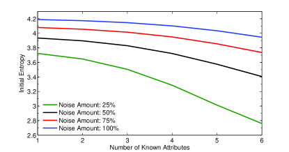
(a) $H_{0}$ vs Intruder’s SK

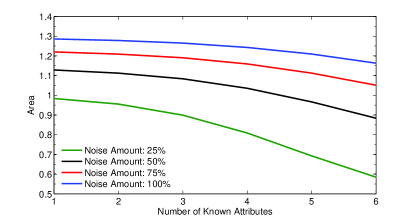
(b) Area vs Intruder’s SK

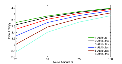
(c) $H_{0}$ vs Noise Amount

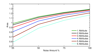
(d) Area vs Noise Amount

Figure 4: SDC: Noise Addition, Dataset: PUMS.

References

- [1] Public Use Microdata Sample (pums), 2006.
- [2] Adam, N.R., John C. Worthmann, J.C.: Security-control methods for statistical databases: a comparative study, ACM Comput. Surv. 21(4), 515–556, 1989.
- [3] Blake, C.L.: Wine Recognition Data, 1998.
- [4] Brankovic, L. and Estivill-Castro, V.: Privacy Issues in Knowledge Discovery and Data Mining. In Proceedings of the Australian Institute of Computer Ethics Conference (AICE1999), 89–99, 1999.
- [5] Brankovic, L., Giggins, H.: Security, privacy, and trust in modern data management, Data-Centric Systems and Applications, ch. Statistical Database Security, pp. 167–181, Springer Berlin Heidelberg, 2007.
- [6] Brankovic, L., Horak, P., Miller, M.: An Optimization Problem in Statistical Databases, SIAM Journal on Discrete Mathematics 13(3), 46–353, 2000.
- [7] Brankovic, L., Horak, P., Miller, M., Wrightson, G.: Usability of Compromise-Free Statistical Databases for Range Sum Queries. In Proceedings of the 9th International Conference on Scientific and Statistical Database Management, IEEE Computer Society, August 11-13, Olympia, Washington, 144–154, 1997.
- [8] Brankovic, L., Lopez, N., Miller, M., Sebe, F.: Triangle randomization for social network data anonymization. Ars Mathematica Contemporanea, 7(2), 461–477, 2014.
- [9] Brankovic, L., Miller, M., Siran, J.: Range Query Usability of Statistical Databases. International Journal of Computer Mathematics, 79(12), 1265–1271, 2002.
- [10] Brankovic, L.: Usability of secure statistical databases. PhD Thesis, Newcastle, Australia, 1998.
- [11] Brankovic, L., Siran, J.: 2-Compromise Usability in 1-Dimensional Statistical Databases. In Proceedings of COCOON2002, H. Ibarra and L. Zhang (Eds.), LNCS 2387, 448–455, 2002.
- [12] Brankovic, L., Miller, M., Siran, J.: Usability of k-compromise-free statistical databases. Proceedings of the 11th Australasian Workshop on Combinatorial Algorithms (AWOCA2000), Hunter Valley, 159–166, 2000.
- [13] Brankovic, L., Islam, Md.Z., Giggins, H.:Security, privacy, and trust in modern data management, Data-Centric Systems and Applications, ch. Privacy-Preserving Data Mining, 151–165, Springer Berlin Heidelberg, 2007.
- [14] Denning, D.E.: Cryptography and data security. Addison-Wesley Longman Publishing Co., Inc., Boston, MA, USA, 1982.
- [15] Duncan, G.T., Lambert, D.: Disclosure-limited data dissemination. Journal of the American Statistical Association, 81, 10–28, 1986.
- [16] Dwork, C.: Differential privacy. In Proceedings of the 33rd International Colloquium on Automata, Languages and Programming (ICALP), 10-14 July, Venice, 1–12, 2006.
- [17] Estivill-Castro, V., Brankovic, L.: Data Swapping: Balancing Privacy Against Precision in Mining for Logic Rules. In Proceedings of Data Warehousing and Knowledge Discovery (DaWaK99), LNCS 1676, 389–399, 1999.
- [18] Estivill-Castro, V., Brankovic, L. and Dowe, D.L.: Privacy in Data Mining. Privacy - Law and Policy Reporter, 9(3), 33–35, 1999.
- [19] Fuller, W.A.: Masking procedures for microdata disclosure limitation. Journal of Official Statistics, 9(2), 383–406, 1993.
- [20] Fung, C.C.M., Wang, K., Chen, R., Yu, P.S.: Privacy-Preserving Data Publishing: A Survey of Recent Developments. ACM Computing Surveys, 42(4), Article 14, 14.2–14.53, 2010.
- [21] Horak, P., Brankovic, L., Miller, M.: A Combinatorial Problem in Database Security. Discrete Applied Mathematics 91(1-3), 119–126, 1999.
- [22] Islam, Md.Z., Barnaghi, P.M., Brankovic, L.: Measuring Data Quality: Predictive Accuracy vs. Similarity of Decision Trees. In Proceedings of the 6th International Conference On Computer And Information Technology (ICCIT2003), December, Dhaka, Bangladesh, 457–462, 2003.
- [23] Islam, Md.Z., Brankovic, L.: Noise Addition for Protecting Privacy in Data Mining. In Proceedings of the 6th Engineering Mathematics and Applications Conference (EMAC2003), Sydney, 85–90, 2003.
- [24] Islam, Md.Z., Brankovic, L.: Detective: A Decision Tree Based Categorical Value Clustering And Perturbation Technique In Privacy Preserving Data Mining. In Proceedings of the 3rd International IEEE Conference On Industrial Informatics (Indin2005), Perth, Australia, 701-708, 2005.
- [25] Kim, J.J.: A method for limiting disclosure in microdata based on random noise and transformation. Proceedings of the Section on Survey Research Methods, American Statistical Association, 303–308, 1986.
- [26] Kim, J.J., Winkler, W.E.: Masking microdata files. Proceedings of the Section on Survey Research Methods, American Statistical Association, 114–119, 1995.
- [27] Lambert, D.: Measures of disclosure risk and harm. Journal of Official Statistics, 9,313–331, 1993.
- [28] King, T., Brankovic, L., Gillard, P.: Perspectives of Australian adults about protecting the privacy of their health information in statistical databases, International Journal of Medical Informatics, 81(4), 2012, pp. 279–89.
- [29] Li, N., Li, T., Venkatasubramanian, S.: t-closeness: Privacy beyond k-anonymity and l-diversity. In Proceedings of IEEE International Conference on Data Engineering, 2007.
- [30] Machanavajjhala, A., Kifer, D., Gehrke, J., Venkitasubramaniam, M.: l-diversity: Privacy beyond k-anonymity. ACM Trans. Knowl. Discov. Data 1, 2007.
- [31] Oganian, A., Domingo-Ferrer, J.: A posteriori disclosure risk measure for tabular data based on conditional entropy. SORT - Statistics and Operations Research Transactions, 27(2), 175–190, 2003.
- [32] Samarati, P., Sweeney, L.: Protecting privacy when disclosing information: k-anonymity and its enforcement through generalization and suppression. Technical Report SRI-CSL-98-04, SRI Computer Science Laboratory, Palo Alto, CA., 1998.
- [33] Sankar, L., Rajagopalan, S.R., Poor, H.V.: Utility-Privacy Tradeoffs for Databases: An Information-theoretic Approach. IEEE Transactions on Information Forensics and Security, Special Issue on Privacy and Trust Management in the Cloud and Distributed Data Systems, 9(6), 838–852, 2013.
- [34] Skinner, C.J., Elliot, M.J.: A measure of disclosure risk for microdata. Journal of the Royal Statistical Society 64(4), 855–867, 2002.
- [35] Spruill, N.L.: Measures of confidentiality. Statistics of Income and Related Administrative Record Research, 131–136, 1982.
- [36] Sramka, M., Safavi-Naini, R., Denzinger, J., Askari, M.: A Practice-oriented Framework for Measuring Privacy and Utility in Data Sanitization Systems. In Proceedings of EDBT/ICDT2010 Workshops, March 22-26, Lausanne, Switzerland, 315–333, 2010.
- [37] Tendick, P.: Optimal noise addition for preserving confidentiality in multivariate data. Journal of Statisical Planning and Inference 27, 341–353, 1991.
- [38] Trottini, M., Fienberg, S.E.: Modelling user uncertainty for disclosure risk and data utility. International Journal of Uncertainty, Fuzziness and Knowledge-Based Systems 10(5), 511–527, 2002.
- [39] Truta, T.M., Fotouhi, F., Barth-Jones, D.: Disclosure risk measures for the sampling disclosure control method. SAC ’04: Proceedings of the 2004 ACM symposium on Applied computing, March, NY, USA, 301–306, 2004.
- [40] Willenborg, L., de Waal, T.: Elements of statistical disclosure control. Lecture Notes in Statistics, 155, Springer-Verlag, New York, 2001.
- [41] Winkler, W.E.: Privacy in statistical databases, ch. Masking and Re-identification Methods for Public-Use Microdata: Overview and Research Problems, pp. 231–246, Springer Berlin Heidelberg, 2004.
- [42] Wolberg, W.H., Street, W.N., Mangasarian, O.L.: Wisconsin Diagnostic Breast Cancer, 1995.
- [43] Yancey, W.E., Winkler, W.E., Creecy, R.H.: Disclosure risk assessment in perurbative microdata protection. Lecture Notes in Computer Science: Inference Control in Statistical Databases, Springer, 2002.