Inflation of small true vacuum bubble by quantization of Einstein$-$Hilbert action

Abstract

We study the quantization of the Einstein$-$Hilbert action for a small true vacuum bubble without matter or scalar field. The quantization of action induces an extra term of potential called quantum potential in Hamilton$-$Jacobi equation, which gives expanding solutions, including the exponential expansion solutions of the scalar factor $a$ for the bubble. We show that exponential expansion of the bubble continues with a short period, no matter whether the bubble is closed, flat, or open. The exponential expansion ends spontaneously when the bubble becomes large, that is, the scalar factor $a$ of the bubble approaches a Planck length $l_{p}$. We show that it is the quantum potential of the small true vacuum bubble that plays the role of the scalar field potential suggested in the slow-roll inflation model. With the picture of quantum tunneling, we calculate particle creation rate during inflation, which shows that particles created by inflation have the capability of reheating the universe.

I Introduction

The inflationary cosmology model by Starobinsky aas79 ; aas80 and Guth ahg81 presents a way to resolve cosmological puzzles of the flatness, horizon and the primordial monopole. The recent detection of B modes in the polarization of the cosmic microwave background by BICEP2 par14 gives a solid evidence for inflationary theory of cosmology. In Guth’s original work, inflation was regarded as a delayed first-order phase transition from the supercooled false vacuum to the lower energy true vacuum. It was soon realized that such a cosmological model has a serious problem called the graceful exit problem. Soon after that, slow-roll inflation model was suggested to overcome this problem al821 ; al822 ; as82 .

The slow-roll model suggested by Linde al821 ; al822 and Albrecht and Steinhardt as82 is based on the symmetry breaking mechanism called Coleman$-$Weinberg mechanism cw73 that allows the phase transition to occur by forming bubbles, while the potential barrier at low temperature is very small. The essence of the slow-roll model is the assumption of the existence of a scalar field $\varphi$, or called inflaton, that makes the value of the potential $V(\varphi)$ be very large but quite flat at the beginning. With the scalar field rolling very slowly down the potential, the bubble experiences a nearly exponential expansion before the field changes very much. However, scientists do not know what the scalar field exactly is until now. A possible candidate is the Higgs field, while the energy Higgs boson is so far from that of inflaton.

It is widely believed that true vacuum without matter or scalar field cannot expand, at least it has no inflationary solution to create the universe bd12 . That is the reason why scientists have to assume the existence of scalar field in inflation theory. Recently, with the de Broglie$-$Bohm quantum trajectory theory and Wheeler$-$DeWitt equation (WDWE), we have proven there are exponential expansion solutions of scalar factor $a$ for a small true vacuum bubble when the operator ordering factor takes a specific value $p=-2$ (or 4 for equivalence), which shows the possibility of spontaneous creation of the universe from nothing, in principle our14 .

In this paper, we extend our previous study on the inflation for a small true vacuum bubble by quantizing its Einstein$-$Hilbert action. When the action of the small true vacuum bubble is quantized with de Broglie$-$Bohm quantum trajectory method, it induces an extra term, usually called quantum potential, in the Hamilton$-$Jacobi equation. The quantization of the action for a small true vacuum bubble can give an exponential expansion solution of the scalar factor $a$ of the bubble with specific ordering factor $p$. We show it is the quantum potential that provides the power for inflation, so that the assumption of the existence of scalar field $\varphi$ in the slow-roll model is not necessary. Numerical solutions show that the Hubble parameter is almost a constant as $H(t)\sim 1/t_{p}$ when the universe is very small ($a\lesssim l_{p}$). The value of Hubble parameter decreases rapidly when the universe becomes large ($a>l_{p}$), and thus the inflation ends. Quantum tunneling method is applied to calculating particle creation rate during inflation, which shows particles created by inflation have the capability of reheating the universe.

II WDWE for a true vacuum bubble

Heisenberg’s uncertainty principle indicates that a small true vacuum bubble can be created probabilistically in a metastable false vacuum, in principle. In fact, it is important to study the behaviors of the small true vacuum bubble after its formation, rather than the process of bubble formation. The small true vacuum bubble can be described by a minisuperspace model npn00 ; npn12 ; apk97 with one single parameter of the scale factor $a$ since it only has one degree of freedom, the bubble radius. The Einstein$-$Hilbert action for the vacuum bubble can be written as

$$S=\frac{c^{3}}{16\pi G}\int\mathcal{R}\sqrt{-g}d^{4}x,$$ (1)

where $c$ is speed of light and $G$ is the gravitational constant. The bubble may be homogeneous and isotropic since it is true vacuum bubble. So, the metric of the bubble in the minisuperspace model is given by

$$ds^{2}=\sigma^{2}\left[-N^{2}(t)c^{2}dt^{2}+a^{2}(t)d\Omega_{3}^{2}\right].$$ (2)

Here, $d\Omega_{3}^{2}=dr^{2}/(1-kr^{2})+r^{2}(d\theta^{2}+\sin^{2}\theta d\phi^{2})$ is the metric on a unit three-sphere, $N(t)$ is an arbitrary lapse function, and $\sigma^{2}=2/3\pi$ is a normalizing factor chosen for later convenience. It should be noted that $r$ is dimensionless and the scale factor $a(t)$ has length dimension Weinberg . From Eq. (2), we can get $\sqrt{-g}=N\sigma^{4}ca^{3}$, and the scalar curvature is given by

$$\mathcal{R}=6\frac{\ddot{a}}{\sigma^{2}c^{2}N^{2}a}+6\frac{\dot{a}^{2}}{\sigma^{2}c^{2}N^{2}a^{2}}+\frac{6k}{\sigma^{2}a^{2}}.$$ (3)

Inserting Eqs. (2) and (3) into Eq. (1), we can get

$$S =\frac{6\sigma^{2}Nc^{4}}{16\pi G}\int\left(\frac{a^{2}\ddot{a}}{N^{2}c^{2}}+\frac{a\dot{a}^{2}}{N^{2}c^{2}}+ka\right)d^{4}x,$$

$$=\frac{6\sigma^{2}Nc^{4}V}{16\pi G}\int\left(\frac{a^{2}\ddot{a}}{N^{2}c^{2}}+\frac{a\dot{a}^{2}}{N^{2}c^{2}}+ka\right)dt,$$

$$=\frac{Nc^{4}}{2G}\int\left(-\frac{a\dot{a}^{2}}{N^{2}c^{2}}+ka\right)dt.$$

The Lagrangian of the bubble can thus be written as

$$\mathcal{L}=\frac{Nc^{4}}{2G}\left(ka-\frac{a\dot{a}^{2}}{N^{2}c^{2}}\right),$$ (4)

where the dot denotes the derivative with respect to time, $t$, and the momentum $p_{a}$ is

$$p_{a}=\frac{\partial\mathcal{L}}{\partial\dot{a}}=-\frac{c^{2}a\dot{a}}{NG}.$$

The Hamiltonian can be expressed by Lagrangian $\mathcal{L}$ and momentum $p_{a}$ in the canonical form:

$$\mathcal{H=}p_{a}\dot{a}-\mathcal{L}.$$

Taking $N=1$, we can get the Hamiltonian

$$\mathcal{H=-}\frac{1}{2}\left(\frac{Gp_{a}^{2}}{c^{2}a}+\frac{c^{4}ka}{G}\right).$$

In quantum cosmology theory, the evolution of the universe is completely determined by its quantum state that should satisfy the WDWE. With $\mathcal{H}\Psi=0$ and $p_{a}^{2}=-\hbar^{2}a^{-p}\frac{\partial}{\partial a}(a^{p}\frac{\partial}{\partial a})$, we get the WDWE for the true vacuum bubble bd67 ; swh84 ; av94 :

$$\left(\frac{\hbar^{2}}{m_{p}}\frac{1}{a^{p}}\frac{\partial}{\partial a}a^{p}\frac{\partial}{\partial a}-\frac{E_{p}}{l_{p}^{2}}ka^{2}\right)\psi(a)=0.$$ (5)

Here, $k=1,0,-1$ are for spatially closed, flat, and open bubbles, respectively. The factor $p$ represents the uncertainty in the choice of operator ordering. $m_{p}$, $E_{p}$, $l_{p}$, and $t_{p}$ are Planck mass, Planck energy, Planck length, and Planck time, respectively.

III Quantization of the action

Mathematically, a complex function $\psi(a)$ in Eq. (5) can be rewritten as

$$\psi(a)=R(a)\exp(iS(a)/\hbar),$$ (6)

where $R$ and $S$ are real functions. Inserting $\psi(a)$ into Eq. (5) and separating the equation into real and imaginary parts, we get two equations bd52 ; prh93 :

$$\frac{\hbar}{m_{p}}\left(S^{\prime\prime}+2\frac{R^{\prime}S^{\prime}}{R}+\frac{p}{a}S^{\prime}\right) =0,$$ (7)

$$\frac{(S^{\prime})^{2}}{m_{p}}+V+Q =0.$$ (8)

Here, $V(a)=E_{p}ka^{2}/l_{p}^{2}$ is the classical potential of the minisuperspace, the prime denotes derivatives with respect to $a$, and $Q(a)$ is the quantum potential, which is given by

$$Q(a)=-\frac{\hbar^{2}}{m_{p}}\left(\frac{R^{\prime\prime}}{R}+\frac{p}{a}\frac{R^{\prime}}{R}\right).$$ (9)

It is easy to verify that Eq. (7) is the continuity equation our14 ; av88 . Eq. (8) is similar to the classical Hamilton$-$Jacobi equation, supplemented by an extra term called quantum potential $Q(a)$. $R$ and $S$ in Eq. (8) can be obtained conveniently from $\psi(a)$ by solving Eq. (5) with relations:

$$\psi(a) =U+iW=R(a)\exp(iS(a)/\hbar),$$ (10)

$$R^{2} =U^{2}+W^{2},\,\,\,S=\hbar\tan^{-1}(W/U).$$ (11)

It is interesting that the Einstein$-$Hilbert action of the true vacuum bubble in Eq. (1) has been quantized in Eq. (11). The quantization of the action gives an extra term $Q(a)$ in Eq. (8), which determines quantum behaviors of the small true vacuum bubble rv14 ; ad14 ; mvj14 . It is clear that a classical true vacuum bubble cannot expand, while, as we show below, a quantized small true vacuum bubble has expanding solutions, including exponential expansion solutions.

By analogy with cases of non-relativistic particle physics and quantum field theory in flat space$-$time, quantum trajectories can be obtained from the guidance relation lpg93 ; npn00 ,

$$\frac{\partial\mathcal{L}}{\partial\dot{a}} =\frac{-c^{2}}{G}a\dot{a}=\frac{\partial S}{\partial a}\,,$$ (12)

$$\dot{a} =-\frac{G}{c^{2}a}\frac{\partial S}{\partial a}\,.$$ (13)

Eq. (13) is a first-order differential equation, so the 3-metric for all values of the parameter $t$ can be obtained by integration. With Eqs. (8) and (13), we can get the Hubble parameter of the bubble:

$$H(t)=\frac{\dot{a}}{a}=\frac{G}{c^{2}}\frac{\sqrt{-m_{p}(Q+V)}}{a^{2}}.$$ (14)

Alternatively, the Hubble parameter can also be obtained from Eqs. (11) and (13). These two methods are equivalent.

IV Expansion solutions of quantized true vacuum bubbles

In this section, we briefly review how to solve the WDWE of the bubble with $k=1,-1,0$, respectively. The quantized action and hence the evolution equations of the scalar factor $a(t)$ of the bubble can be obtained with the wave functions of the bubble our14 .

IV.1 The closed bubble

In this case $k=1$, the analytic solution of Eq. (5) is

$$\psi(a)=\left(\frac{a}{l_{p}}\right)^{\frac{1-p}{2}}\left[ic_{1}I_{\nu}\left(\frac{a^{2}}{2l_{p}^{2}}\right)-c_{2}K_{\nu}\left(\frac{a^{2}}{2l_{p}^{2}}\right)\right],$$ (15)

where $I_{\nu}$’s are modified Bessel functions of the first kind, $K_{\nu}$’s are the modified Bessel function of the second kind, the coefficients $c_{1}$ and$\ c_{2}$ are arbitrary constants, and $\nu=|1-p|/4$. Generally speaking, the wave function of the bubble should be complex. Specially, if the wave function of the universe is pure real or pure imaginary, we have $S^{\prime}=0$ so there are no expansion solutions. For simplicity, we set $c_{1}$ and$\ c_{2}$ as real numbers to find the expansion solutions.

Using Eqs. (10) and (11), we can get

$$S=\hbar\tan^{-1}\left[-\frac{c_{1}}{c_{2}}\frac{I_{\nu}\left(\frac{a^{2}}{2l_{p}^{2}}\right)}{K_{\nu}\left(\frac{a^{2}}{2l_{p}^{2}}\right)}\right]$$

and

$$R=a^{(1-p)/2}\sqrt{\left[c_{1}I_{\nu}\left(\frac{a^{2}}{2l_{p}^{2}}\right)\right]^{2}+\left[c_{2}K_{\nu}\left(\frac{a^{2}}{2l_{p}^{2}}\right)\right]^{2}}\,\,.$$

Here, we omit the sign “$\pm$” and “$l_{p}$” in front of $R$, since they don’t affect the value of $Q(a)$ in Eq. (9). For small arguments $0<x\ll\sqrt{\nu+1}$, Bessel functions take the following asymptotic forms:

$$I_{\nu}(x)\sim\frac{1}{\Gamma(\nu+1)}\left(\frac{x}{2}\right)^{\nu}$$

and

$$K_{\nu}(x)\sim\frac{\Gamma(\nu)}{2}\left(\frac{2}{x}\right)^{\nu},\,\,\,\,\nu\neq 0,$$

where $\Gamma(z)$ is the Gamma function. It is easy to get

$$S(a\ll l_{p})\approx-\frac{2\hbar c_{1}}{c_{2\Gamma(\nu)\Gamma(\nu+1)}}\left(\frac{a^{2}}{4l_{p}^{2}}\right)^{2\nu},\,\,\,\,\,\,\nu\neq 0.$$

Using the guidance relation (13), we can get the trajectories for any small scale factor

$$a(t)=\left\{\begin{aligned} &\left[\frac{(3-4\nu)\lambda(\nu)}{3}(t+t_{0})\right]^{\frac{1}{3-4\nu}},\,\,\,\,\,\,\nu\neq 0,\,\,\frac{3}{4},\\ &e^{\lambda(3/4)(t+t_{0})},\,\,\,\,\,\,\,\,\,\,\,\,\,\,\,\,\,\,\,\,\,\,\,\,\,\,\,\,\,\,\,\,\,\,\,\,\,\,\,\,\,\,\,\,\,\,\,\,\,\nu=\frac{3}{4},\\ \end{aligned}\right.$$

where $\lambda(\nu)=6c_{1}/(t_{p}4^{2\nu}c_{2}\Gamma(\nu)\Gamma(\nu+1))$ has dimension of $T^{-1}$. For the case of $p=1$ (i.e., $\nu=0$), there is no expansion solution for the WDWE no matter whether the bubble is closed, flat, or open.

It is clear that only the ordering factor takes the value $p=-2$ (or $p=4$ for equivalence), i.e., $\nu=3/4$, has the scale factor $a(t)$ an exponential behavior. In this case, the quantum potential of the small true vacuum bubble is

$$Q(a\rightarrow 0)=-\frac{E_{p}}{l_{p}^{2}}\left(a^{2}+\frac{\lambda(3/4)^{2}}{c^{2}}a^{4}\right).$$ (16)

We find that the first term in quantum potential $Q(a\rightarrow 0)$ exactly cancels the classical potential $V(a)=E_{p}a^{2}/l_{p}^{2}$. The effect of the second term $-E_{p}\lambda(3/4)^{2}a^{4}/l_{p}^{2}$ is quite similar to that of the scalar field potential in hhh12 or the cosmological constant in dhc05 for inflation. Numerically solutions for the evolution of Hubble parameter $H=\dot{a}/a$ of the closed bubble will be discussed later.

IV.2 The open bubble

For the case $k=-1$, the analytic solution of Eq. (5) is found to be

$$\psi(a)=\left(\frac{a}{l_{p}}\right)^{\frac{1-p}{2}}\left[ic_{1}J_{\nu}\left(\frac{a^{2}}{2l_{p}^{2}}\right)+c_{2}Y_{\nu}\left(\frac{a^{2}}{2l_{p}^{2}}\right)\right],$$ (17)

where $J_{\nu}$’s are Bessel functions of the first kind, and $Y_{\nu}$’s are Bessel function of the second kind and $\nu=|1-p|/4$. With the relations in Eqs. (10) and (11), we can get

$$S=\hbar\tan^{-1}\left[\frac{c_{1}}{c_{2}}\frac{J_{\nu}(\frac{a^{2}}{2l_{p}^{2}})}{Y_{\nu}(\frac{a^{2}}{2l_{p}^{2}})}\right],$$

and

$$R=a^{(1-p)/2}\sqrt{\left[c_{1}J_{\nu}\left(\frac{a^{2}}{2l_{p}^{2}}\right)\right]^{2}+\left[c_{2}Y_{\nu}\left(\frac{a^{2}}{2l_{p}^{2}}\right)\right]^{2}}\,\,.$$

For small arguments $0<x\ll\sqrt{\nu+1}$, Bessel functions take the following asymptotic forms, $J_{\nu}(x)\sim(x/2)^{\nu}/\Gamma(\nu+1)$, and $Y_{\nu}(x)\sim-\Gamma(\nu)2^{\nu-1}/x^{\nu}$ for $(\nu\neq 0)$. So, we have

$$S(a\ll 1)\approx-\frac{\hbar\pi c_{1}}{c_{2\Gamma(\nu)\Gamma(\nu+1)}}\left(\frac{a^{2}}{4l_{p}^{2}}\right)^{2\nu},\,\,\,\,v\neq 0.$$

and

$$a(t)=\left\{\begin{aligned} &\left[\frac{(3-4\nu)\bar{\lambda}(\nu)}{3}(t+t_{0})\right]^{\frac{1}{3-4\nu}},\,\,\,\,\,\nu\neq 0,\,\,\frac{3}{4}\\ &e^{\bar{\lambda}(3/4)(t+t_{0})},\,\,\,\,\,\,\,\,\,\,\,\,\,\,\,\,\,\,\,\,\,\,\,\,\,\,\,\,\,\,\,\,\,\,\,\,\,\,\,\,\,\,\,\,\,\,\,\,\nu=\frac{3}{4},\end{aligned}\right.$$

where $\bar{\lambda}(\nu)=3\pi c_{1}/(t_{p}4^{2\nu}c_{2}\Gamma(\nu)\Gamma(\nu+1))$.

Similarly, the scale factor $a(t)$ has an exponential behavior for the special case of $p=-2$ (or 4). In this case, the quantum potential for the bubble can be obtained as

$$Q(a\rightarrow 0)=\frac{E_{p}}{l_{p}^{2}}\left(a^{2}-\frac{\bar{\lambda}(3/4)^{2}}{c^{2}}a^{4}\right).$$ (18)

The terms $a^{2}$ in quantum potential $Q(a\rightarrow 0)$ and classical potential $V(a)$ cancel each other exactly. Thus, it is the second term $-E_{p}\bar{\lambda}(3/4)^{2}a^{4}/l_{p}^{2}c^{2}$ in quantum potential $Q(a\rightarrow 0)$ that causes the exponential expansion.

IV.3 The flat bubble

For the case of $k=0$, the analytic solution of Eq. (5) is

$$\psi(a)=\frac{ic_{1}}{1-p}\left(\frac{a}{l_{p}}\right)^{1-p}-c_{2},$$ (19)

where $p\neq 1$, and hence

$$S =\tan^{-1}\left[-\frac{c_{1}}{c_{2}(1-p)}\left(\frac{a}{l_{p}}\right)^{1-p}\right],\,\,\,\,p\neq 1,$$

$$R =\sqrt{c_{2}^{2}+\left(\frac{c_{1}}{1-p}\frac{a^{1-p}}{l_{p}^{1-p}}\right)^{2}},\,\,\,\,p\neq 1.$$

With the guidance relation (13), we can get the form of time-dependent scalar factor $a(t)$ as

$$a(t)=\left\{\begin{aligned} &\left[\frac{c_{1}}{c_{2}}(3-|1-p|)\frac{(t+t_{0})}{t_{p}}\right]^{\frac{1}{3-|1-p|}},\,|1-p|\neq 0,3,\\ &e^{\frac{c_{1}}{c_{2}}\frac{(t+t_{0})}{t_{p}}},\,\,\,\,\,\,\,\,\,\,\,\,\,\,\,\,\,\,\,\,\,\,\,\,\,\,\,\,\,\,\,\,\,\,\,\,\,\,\,\,\,\,\,\,\,\,\,\,\,\,\,\,\,\,\,\,\,\,\,\,\,\,\,\,|1-p|=3.\end{aligned}\right.$$

It is clear that only the ordering factor takes the value $p=-2$ (or 4), will the small true vacuum bubble have the exponential expansion solutions. The accompanying quantum potential for the flat bubble is $Q(a\rightarrow 0)=-E_{p}(c_{1}/c_{2})^{2}a^{4}/l_{p}^{4}$, while the classical potential is $V(a)=0$ on this condition. This definitely means that it is the quantum potential $Q(a)$ that is the origin of exponential expansion for the small true vacuum bubble.

V Hubble parameter and quantum potential

From the discussion above, we can see that both Hubble parameter and quantum potential of the bubble depend on three parameters: the operator ordering $p$, the boundary condition $c_{1}/c_{2}$, and the initial condition $a_{0}$. In this section, we study the time-dependent evolutions of Hubble parameters and quantum potential numerically with different $p$ and $c_{1}/c_{2}$.

V.1 Hubble parameter with different $p$

With the real part $R(a)$ of wave function, we can get the value of quantum potential $Q(a)$ using Eq. (9). The evolution of Hubble parameter can thus be obtained from Eq. (14).

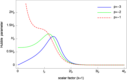
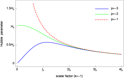
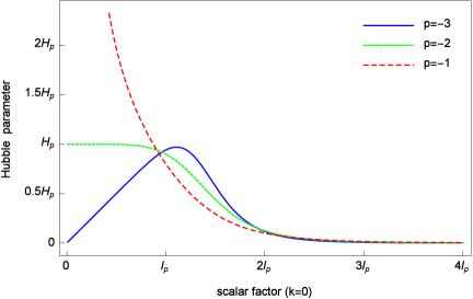
Figure 1: (color online)  Hubble parameters for closed,open and flat bubbles, respectively. Here, we have set $c_{1}/c_{2}=1$.

Detailed calculations show that when the bubble is very small, that is, $a\rightarrow 0$, Hubble parameters are divergent for $\nu<3/4$, and it approaches zero for $\nu>3/4$. Only $\nu$ takes value $\nu=3/4$, that is, $p=-2$ (or 4 for equivalence), has the bubble exponential expansion solutions. In the limit of large bubble, different operator ordering factors give the same behavior of Hubble parameters. Explicitly numerical solutions can be found in Fig. 1. It is clear that the effect of the operator ordering $p$ is significant when the bubble is small (i.e., $a\lesssim l_{p}$), while its effects are too small to be negligible when the bubble becomes large (i.e., $a\gg l_{p}$). In this case, we can conclude that the ordering factor $p$ represents quantum effects of the bubble as described by Eq. (5).

V.2 Quantum potential of a true vacuum bubble

We have shown that the small true vacuum bubble expands exponentially no matter the bubble is closed, open, or flat as long as the ordering factor takes a specific value $p=-2$ (or 4). As discussed previously, it is the quantum potential that provides power for inflation. In the following, we study the evolutions of quantum potential of the bubble with the increase of $a$. For simplicity, we set $p=-2$ and $c_{1}/c_{2}=1$ in numerical solutions.

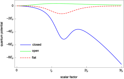
Figure 2: (color online)   The value of quantum potential for the closed, open, and flat bubbles with the variation of $a$.

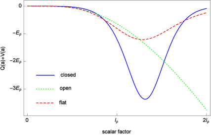
Figure 3: (color online)   The value of quantum potential plus classical potential (that is, the value of $V(a)+Q(a)$) for closed, open, and flat bubbles versus $a$.

In Fig. 2, we find that $Q(a\gg l_{p})\rightarrow 0$ for the open and flat bubbles, which indicates the quantum effects can be neglected when the bubble becomes large enough. For the closed bubble, the asymptotic behavior of its quantum potential is $Q(a\gg 1)\sim-a^{2}$, which exactly cancels the value of classical potential. This indicates that the quantum effect of the closed bubble is significant no matter how large the bubble is. According to the de Broglie$-$Bohm quantum trajectory theory, the closed bubble should be in a steady state in the large limit. Thus, we can conclude that the scale factor $a$ of a small true vacuum bubble stops accelerating when the bubble becomes very large, no matter whether the bubble is closed, open, or flat.

When the bubble is very small, that is, $a\lesssim l_{p}$, the sum of quantum potential plus classical potential is directly proportional to $-a^{4}$, $Q(a)+V(a)\sim-a^{4}$, no matter whether the bubble is closed, open, or flat. As shown in Fig. 3, $Q(a)+V(a)$ changes very slowly when $a$ is small ($a\lesssim l_{p}$), while it decreases quickly when $a$ of the bubble becomes large ($a>l_{p}$), which completely satisfies the slow-roll inflation conditions al821 ; al822 ; as82 . Here, we can conclude that it is the quantum potential that provides the power for the vacuum bubble inflation, which plays the role of the assumed scalar field in the slow-roll inflation theory.

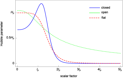
Figure 4: (color online)   The evolution of Hubble parameter with scale factor for closed, open, and flat bubbles, respectively, with the operator ordering factor $p=-2$ and $c1/c2=1$.

Numerical solutions in Fig. 4 show that the Hubble parameter $H$ is almost a constant when the bubble is very small, i.e., $a\ll l_{p}$. For the closed or flat bubbles, Hubble parameters decrease to zero when the scalar factor $a$ becomes large enough ($a\gg 3l_{p}$). For an open large bubble, its Hubble parameter is inverse to $a$ (i.e., $H(a)\sim 1/a$), which means the bubble expands with a constant velocity when the bubble is very large. Then, we can get the conclusion again: the vacuum bubble will stop accelerating when it becomes very large, no matter whether it is closed, flat, or open.

V.3 Hubble parameter with different $c_{1}/c_{2}$

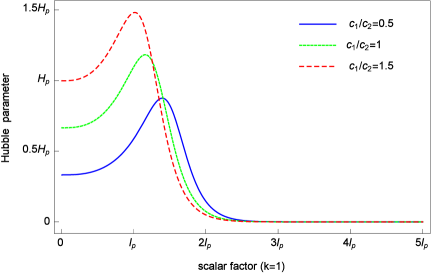
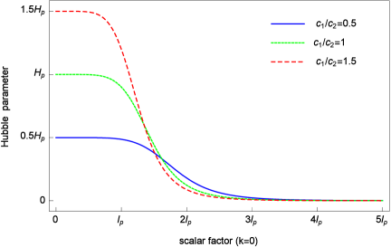
Figure 5: (color online)   Hubble parameter for closed or flat bubbles with different $c_{1}/c_{2}$.

We study the case of inflation solutions ($p=-2$) with different values of $c_{1}/c_{2}$. Numerical solutions in Fig. 5 show that the evolutions of Hubble parameter have similar form with different values of $c_{1}/c_{2}$ for closed or flat vacuum bubble. However, for open bubbles, Fig. 6 shows Hubble parameters decrease with oscillations as $a$ increases when $c_{1}/c_{2}\neq 1$. For a bubble with finite value of $c_{1}/c_{2}$, its Hubble parameter approaches zero when the bubble becomes large enough. The oscillations of quantum potential increases while the oscillations of the companying Hubble parameters decrease with the increase of $a$. This implies that the inflation will exit when the bubble becomes large enough, no matter the bubble is closed, open, or flat.

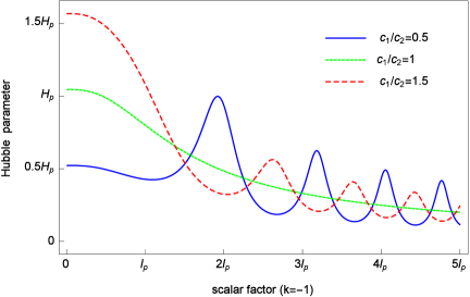
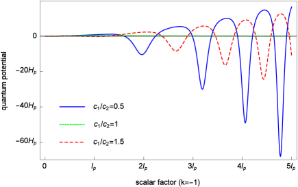
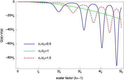
Figure 6: (color online)   Hubble parameters and the accompanying quantum potential for open bubbles with different $c_{1}/c_{2}$.

V.4 The e-folding number

Let us consider how long the inflation sustains. It has been shown above that inflation will exit when the scale factor approaches Planck length, $a\sim l_{p}$. During inflationary stage, we have $a\approx a_{0}e^{Ht}$, where $a_{0}$ is the initial value of $a$ at $t=0$. So, the e-folding number can be obtained as

$$N\sim\ln{\frac{l_{p}}{a_{0}}}\approx Ht_{end}.$$ (20)

The e-folding number $N$ is determined by the initial condition of the bubble, $a_{0}\sim l_{p}e^{-N}$. The early universe has enough time ($t_{end}\approx Nt_{p}$) to maintain inflation as long as $a_{0}$ is small enough. In practice, the standard cosmological model requires the e-folding number $N\gtrsim 60$, which implies that the exponential expansion of the early universe continues at least more than 60 Planck time.

VI Particle creation by inflation

There is no doubt that the space and time of the early universe will emerge by the exponential expansion of the bubble. One may ask an important question how matter appears in the early universe. In the scalar field inflationary model, almost all matter, antimatter, and photons were produced by the energy of scalar field that was released following the phase transition. However, in our calculations, it is the quantum potential that provides the power for inflation. In the following, we show that particles can be created by the exponential expansion of the bubble with quantum tunneling mechanism.

The change of the spacetime metric at the end of inflation will itself create particles due to their coupling to the spacetime curvature, which has been discussed in many papers lp69 ; asl78 ; ndb82 ; lhf87 . In 2000, Parikh and Wilczek applied quantum tunneling method to Hawking radiation mkp00 . This method gives a nonthermal spectrum which has been used to recover the lost information in Hawking radiation zbc09a ; zczy13 . Another method called Hamilton$-$Jacobi method kt99 ; lgr11 has also been suggested to obtain the tunneling probability. We apply this method to inflationary universe which has a de Sitter spacetime (the metric for a free observer who stays in an exponential expansion spacetime) to calculate particle creation.

VI.1 The Friedmann$-$Robertson$-$Walker (FRW) spacetime

The line element of a homogeneous and isotropic universe can be written as

$$ds^{2}=-dt^{2}+a^{2}(t)d\Omega^{3}.$$ (21)

The metric above is equivalent to that in Eq. (2). Here, we omit the normalizing factor $\sigma$ in Eq. (2), because the normalizing factor doesn’t influence our calculation. During the inflationary phase, the scale factor takes the form $a(t)=e^{Ht}$, and $H=\overset{.}{a(t)}/a(t)$ is Hubble parameter. For simplicity, we set $\hbar=c=k_{B}=1$ hereafter.

The frame of an observer at some spacetime point in the de Sitter phase is described by the static coordinates. The static de Sitter coordinates $(\widetilde{t},\widetilde{r},\theta,\varphi)$ are given in terms of the FRW coordinates $(t,r,\theta,\varphi)$ by rhb85

$$\widetilde{r} =e^{Ht}r,$$ (22)

$$\widetilde{t} =-\frac{1}{2H}\ln\left[e^{-2Ht}-(rH)^{2}\right].$$ (23)

These relations are valid in the region $\widetilde{r}<1/H$. From Eqs. (22) and (23), we can get

$$dt =d\widetilde{t}-\frac{H\widetilde{r}}{1-H^{2}\widetilde{r}^{2}}d\widetilde{r},$$ (24)

$$dr =-\frac{e^{-H\widetilde{r}}H\widetilde{r}}{\sqrt{1-H^{2}\widetilde{r}^{2}}}d\widetilde{t}+\frac{e^{-H\widetilde{r}}}{\left(1-H^{2}\widetilde{r}^{2}\right)^{3/2}}d\widetilde{r}.$$ (25)

Inserting Eqs. (22)$-$(25) into FRW line element (21), we can get the static de Sitter metric:

$$ds^{2}=-(1-H^{2}\widetilde{r}^{2})d\widetilde{t}^{2}+(1-H^{2}\widetilde{r}^{2})^{-1}d\widetilde{r}^{2}+\widetilde{r}^{2}d\Omega^{2}.$$ (26)

Here, we have set $k=0$ for simplicity (it has been discussed that $k$ is unimportant for particle creation during inflation sd12 ; lgr11 ). Taking the substitution $H^{2}\rightarrow 2M/\widetilde{r}^{3}$, we can find that this metric is similar to the usual Schwarzschild metric, and the horizon is located at $\widetilde{r}_{H}=1/H$.

The static metric has a limitation that it is only valid up to the horizon, since there is a singularity at $\widetilde{r}_{H}=1/H$. It is well known that Painlevé metric can describe across-horizon phenomena of a black hole mkp00 ; lgr11 . Then, we translate the de Sitter metric to Painlevé-type metric via the transformations

$$d\widetilde{t}=dT-\frac{H\widetilde{r}}{1-H^{2}\widetilde{r}^{2}}d\widetilde{r}.$$

With this choice, the metric (26) reads

$$ds^{2}=-(1-H^{2}\widetilde{r}^{2})dT^{2}-2H\widetilde{r}dTd\widetilde{r}+d\widetilde{r}^{2}+\widetilde{r}^{2}d\Omega^{2}.$$ (27)

At a fixed time, the spatial geometry described by (27) is Euclidean, while at any fixed radius, the boundary geometry is the same as that in (26). The metric is no more singular at the horizon $\widetilde{r}_{H}$. Furthermore, the spacetime is stationary, but no more static. The $T$ coordinate is nothing more than the proper time along a radial geodesic worldline, such as a free-falling observer.

VI.2 Tunneling across the cosmological horizon

The great utility for a coordinate system which is well behaved at the horizon is that one can study across-horizon physics. In this section, we study a scalar field placed in a background spacetime. Physically, these fields come from vacuum fluctuations that permeate the spacetime given by the metric. The minimally coupled Klein$-$Gordon equation for a scalar field $\phi$ of mass $m$ in curved spacetime $g_{\mu\nu}$ has the form ndb82 :

$$\left[\frac{1}{\sqrt{-g}}\partial_{\mu}\left(\sqrt{-g}g^{\mu\nu}\partial_{\nu}\right)-\frac{m^{2}c^{2}}{\hbar^{2}}\right]\phi=0.$$ (28)

Inserting the scalar field in terms of a phase factor as $\phi=\phi_{0}e^{iS(t_{p},\widetilde{r})/\hbar}$ into Eq. (28), and taking the limitation $\hbar\rightarrow 0$, we can get the Hamilton$-$Jacobi equation for the action $S$ of the field $\phi$ in the gravitational background adg10 :

$$g^{\mu\nu}\left(\partial_{\mu}S\right)\left(\partial_{\nu}S\right)+m^{2}=0.$$ (29)

For stationary spacetime, the action $S$ can be split into two part, the time part and space part, $S(T,\widetilde{r})=ET+S_{0}(\widetilde{r})$. In the Wentzel$-$Kramers$-$Brillouin limit, the probability of tunneling is related to the imaginary part of the action for the classically forbidden trajectory mkp00 :

$$\Gamma\sim e^{-2\operatorname{Im}S}.$$ (30)

Applying the stationary Painlevé metric in Eq. (27) to the Hamilton$-$Jacobi in Eq. (29), we can get

$$-E^{2}-2EH\widetilde{r}\partial_{\widetilde{r}}S+(1-H^{2}\widetilde{r}^{2})\left(\partial_{\widetilde{r}}S\right)^{2}+m^{2}=0.$$

In this case, the action $S$ can be obtained as

$$S=\int\frac{EH\widetilde{r}}{1-H^{2}\widetilde{r}^{2}}d\widetilde{r}\pm\int\frac{\sqrt{E^{2}-m^{2}(1-H^{2}\widetilde{r}^{2})}}{1-H^{2}\widetilde{r}^{2}}d\widetilde{r}.$$ (31)

Here, the positive and negative signs indicate ingoing and outgoing particles, respectively. It should be pointed out that the energy of ingoing particle is positive and the energy of outgoing particle is negative, which are different from those in Hawking radiation as tunneling. The contour integral includes a singularity at $\widetilde{r}=1/H$ and it has to be made by going around the pole at singularity. In this way, we can obtain the imaginary part of the ingoing particle as

$$\operatorname{Im}S=\frac{\pi E}{H}.$$

When we consider outgoing particles, a minus sign should be added to the first term in the right of Eq. (31) zbc09b . Similarly, we can get $\operatorname{Im}S=\pi E/H$ for the outgoing particles. Finally, we can obtain the tunneling probability for two channels as

$$\Gamma\sim e^{-\frac{2\pi E}{H}}.$$ (32)

Comparing the tunneling rate with the Boltzmann factor, we find the temperature of the bubble, which is given by

$$T_{H}=\frac{H}{2\pi}.$$ (33)

In principle, the inflationary universe should radiate all particles in the standard model with a black body spectrum. To obtain the radiation rate of fermionic particles across the horizon of de Sitter spacetime, one should replace the Klein$-$Gordon equation with the Dirac equation in curved spacetime, and the similar results as those in Eq. (33) can be obtained lgr11 ; km08 .

VI.3 Reheating

The Hubble constant of the present universe is $H_{now}\approx 2.29\times 10^{-18}\operatorname{s}^{-1}$, so the temperature $T$ at present is about

$$T=\frac{\hbar H_{now}}{2\pi k_{B}}\approx 2.78\times 10^{-30}\operatorname{K}.$$ (34)

This temperature is much less than the temperature of microwave background radiation. Except the inflation period, the universe has a very small Hubble parameter $H\ll 1/t_{p}$, so the effect of particle creation is negligible after the inflation exits.

Let us estimate whether Hawking radiations created by inflation have the capacity of reheating the universe or not. In the minisuperspace model, all observers would see a horizon at $\widetilde{r}_{H}$ and a Hawking temperature $T_{H}$. So, the temperature of the universe is identical everywhere during inflation. Because the Hubble parameter changes slowly, according to the Stephan$-$Boltzmann radiation law, the energy density $\rho_{end}$ at the end of inflationary universe is

$$\rho_{end}=\frac{4\sigma}{c}T_{H}^{4}=\frac{\hbar H^{4}}{240\pi^{2}c^{3}}.$$ (35)

Here, $\sigma=\pi^{2}k_{B}^{4}/60\hbar^{3}c^{2}$ is the Stephan$-$Boltzmann constant. The universe was dominated by radiations after inflation, and then it graded into the stage dominated by matter. Suppose that it was at $t_{m}$ that matter began to dominate the universe with energy density $\rho_{m}$. In the radiation dominance stage, the energy density $\rho\propto a^{-4}$ and the scalar factor $a\propto t^{1/2}$, so we have

$$\frac{\rho_{end}}{\rho_{m}}=\left(\frac{a_{m}}{a_{end}}\right)^{4}=\left(\frac{t_{m}}{t_{end}}\right)^{2}.$$ (36)

In matter dominance phase, the energy density $\rho\propto a^{-3}$ and the scalar factor $a\propto t^{2/3}$, so we have

$$\frac{\rho_{m}}{\rho_{now}}=\left(\frac{a_{now}}{a_{m}}\right)^{3}=\left(\frac{t_{now}}{t_{m}}\right)^{2}.$$ (37)

Combine the Eqs. (36) and (37), we can obtain

$$\frac{\rho_{end}}{\rho_{now}}=\frac{\rho_{end}}{\rho_{m}}\frac{\rho_{m}}{\rho_{now}}=\left(\frac{t_{now}}{t_{end}}\right)^{2}.$$

According to the Planck data, the age of the universe is 13.82 billion years, that is, $t_{now}\approx 4.36\times 10^{17}\operatorname{s}$, and the matter density (including dark matter and ordinary matter) of the present universe is $\rho_{now}\approx\Omega_{m}\rho_{c}\approx 2.6\times 10^{-27}\operatorname{kg}/\operatorname{m}^{3}$. From equation (20), we can get $t_{end}=N/H$. In the standard cosmological model, $N\approx 60$. In our model, it is sound that the Hubble parameter $H$ takes the value $H\sim 1/t_{p}\sim 1.8\times 10^{43}\operatorname{s}^{-1}$. From Eq. (35), we can get

$$\rho_{end}\left(\frac{t_{end}}{t_{now}}\right)^{2}=1.21\times 10^{-25}\operatorname{kg}/\operatorname{m}^{3}.$$

Then, we have $\rho_{end}\left(\frac{t_{end}}{t_{now}}\right)^{2}>\rho_{now}$, which suggests that the particles created by inflation have the capability of reheating the universe and of being the source of the matter in the universe.

The origin of the matter$-$antimatter asymmetry is one of the great questions in cosmology. According to tunneling picture, particle and anti-particle should be created at the same time and with the same quantity. However, there is good evidence that there are no large regions of antimatter at any but cosmic distance scales cas98 ; mar04 . It was Sakharov who first suggested that the baryon density might not represent some sort of initial condition, but might be understandable in terms of microphysical laws sad67 . He listed three ingredients to such an understanding: (1) baryon-number violation, (2) charge parity violation, and (3) departure from thermal equilibrium. If the reheating temperature is greater than the mass of the gauge bosons, one can generate the observed baryon asymmetry by charge parity violation decays of these bosons. Baryon asymmetry can also be generated by the decay of Higgs bosons if the reheating temperature is at least $10^{11}\operatorname{GeV}$ mar04 . In our calculation, the temperature is high enough ($T_{H}\sim 2\times 10^{31}\operatorname{K}$, or the energy scale is about $2\times 10^{18}\operatorname{GeV}$) to satisfy these conditions, so it is possible to generate baryon asymmetry during the inflationary universe.

VII Energy particle conversion

The temperature of inflationary universe can also be obtained by the Unruh effect. The Unruh temperature, derived by William Unruh in 1976 un76 , is the effective temperature experienced by a uniformly accelerating detector in a vacuum field:

$$T=\frac{\kappa}{2\pi},$$ (38)

where $\kappa$ is acceleration. Inserting the surface gravity on horizon into Eq. (38), one can easily recover the result in Eq. (33).

For flat FRW metric, the gravity at $\widetilde{r}$ is rs05

$$\kappa=-\frac{\widetilde{r}}{2}\left(\dot{H}+2H^{2}\right).$$ (39)

Since the horizon is located at $\widetilde{r}=1/H$, we can get $\kappa=-H$. Here, the minus sign indicates that the direction of radiation flux from the cosmological horizon is opposite to the radiation flux from a black hole horizon. For black holes, the positive energy particles escape from the event horizon to asymptotic infinity. However, for the horizon of FRW spacetime, the positive energy particles go inward from the horizon. The temperature is $T=\mid\kappa\mid/2\pi=H/2\pi$ for an empty de Sitter spacetime.

Once there is a particle created by inflation, the spacetime is no longer empty. In this case, the gravity of the particle will affect the cosmological horizon and the surface gravity. When there is a particle with positive energy $\omega$ in de Sitter spacetime, the Einstein field equation reads

$$\left(\frac{\dot{a}}{a}\right)^{2}=\frac{8\pi G}{3}\rho_{\gamma}+\frac{\Lambda}{3},$$ (40)

$$\frac{\ddot{a}}{a}=-\frac{4\pi G}{3}\left(\rho_{\gamma}+3p_{\gamma}\right)+\frac{\Lambda}{3}.$$ (41)

Here, the energy $\omega$ is relativistic particle, so we have $p_{\gamma}=\rho_{\gamma}/3$, and $\rho_{\gamma}=3\omega H_{f}^{3}/4\pi\ll\Lambda/3$. $H_{i}$ represents the Hubble constant for an empty de Sitter spacetime, and $H_{f}$ represents the Hubble constant after the energy $\omega$ emit into de Sitter spacetime. $H_{i}$ can be obtained by setting $\rho_{\gamma}=0$ in Eq. (40) as $H_{i}=\sqrt{\Lambda/3}.$ Using Eqs. (40) and (41), we can get

$$\dot{H_{f}} =-\frac{16\pi G}{3}\rho_{\gamma}=-4G\omega H_{f}^{3},$$ (42)

$$H_{f} =\sqrt{\frac{8\pi G}{3}\rho_{\gamma}+H_{i}^{2}}=\sqrt{2G\omega H_{f}^{3}+H_{i}^{2}}.$$ (43)

When there is a particle $\omega$, the surface gravity on the horizon becomes

$$\kappa_{f}=-\frac{1}{2H_{f}}\left(\dot{H_{f}}+2H_{f}^{2}\right).$$ (44)

Inserting (42) and (43) into (44), and expanding $\kappa$ in power of $\omega$, we can get

$$\mid\kappa_{f}\mid =\frac{H_{i}^{2}}{H_{f}}\approx\frac{H_{i}}{\sqrt{2G\omega H_{i}+1}}$$

$$\approx H_{i}(1-G\omega H_{i}).$$ (45)

Here, we have used the fact that the energy of the tunneled particle $\omega$ is small, and $H_{i}$ and $H_{f}$ only have a tiny difference. The temperature of the universe can thus be obtained as

$$T_{f}=\frac{H_{i}(1-G\omega H_{i})}{2\pi},$$ (46)

which is lower than the temperature of the empty de Sitter spacetime $T_{i}$. This result is physically reasonable because it is consistent with (33) when $\omega\rightarrow 0$. The expression (42) shows that $\dot{H_{f}}<0$, which means the Hubble constant will decrease and the horizon radius expends after the energy $\omega$ enters the cosmological horizon. At the beginning of the particle creation, there were a few particles in space, so the Hubble parameter decrease very slowly. With the time increasing, there are more and more particles created in the space, which induce a rapid decrease of the Hubble parameter and the temperature. In this way, the energy of quantum potential changes to particles by exponential expansion of the space and the inflation turns off.

VIII Discussion and conclusion

For inflation driven by a scalar inflaton field $\phi$, the power spectra of curvature and tensor perturbations are defined as bt06

$$\mathcal{P}_{R} \simeq\left(\frac{V^{3}}{m_{p}^{6}(V^{\prime})^{2}}\right)_{k=aH},$$ (47)

$$\mathcal{P}_{T} \simeq\left(\frac{V}{m_{p}^{4}}\right)_{k=aH},$$ (48)

where $V(\phi)$ is the potential of the scalar inflaton field $\phi$ and the primed means derivative with respect to $\phi$. For the slow-roll inflation model, we have the energy density of the scalar field $\rho=\dot{\phi}^{2}/2+V(\phi)\approx V(\phi)$, and $\rho=3m_{p}^{2}H^{2}/8\pi$. The scalar and tensor perturbations are related by $\mathcal{P}_{T}=r\mathcal{P}_{R}$. Observations par14 tell us that $r\approx 0.2$ and $\mathcal{P}_{R}\approx 10^{-9}$, which yield $\mathcal{P}_{T}\approx 10^{-10}$, $\rho\approx 10^{-10}m_{p}^{4}$, and $H\approx 10^{-5}m_{p}$. We should point out that the result $H\lesssim 10^{-5}m_{p}$ is model dependent. In our inflation model, there is no scalar inflaton field. It is not obvious whether these results can be directly applied to our model or not. So, in our calculation of reheating, $H$ takes a value at Planck scale. How to determine the value of Hubble parameter will be studied in future.

In summary, we have discussed the expansion solutions of a small true vacuum bubble. We found there is an extra term called quantum potential in the Hamilton$-$Jocabi equation after the action of the bubble was quantized. The exponential expansion solutions of the bubble can be obtained with a specific operator ordering $p=-2$ (or 4). Numerical calculations show that the Hubble parameter $H=\dot{a}/a\sim 1/t_{p}$ during the inflationary stage, and the exponential expansion will end when the scale factor approaches $a\sim l_{p}$. The value of quantum potential plus classical potential is proportional to $a^{4}$ for a small bubble ($a\lesssim l_{p}$), while it decreases rapidly after the bubble grows up ($a>l_{p}$). This indicates that the quantum potential of the vacuum bubble satisfies the conditions required by slow-roll inflation. Thus, we can conclude that it is the quantum potential of the vacuum bubble that plays the role of the scalar field potential assumed in the slow-roll inflation model.

We have also studied particle creation by inflation with the picture of quantum tunneling through the cosmological horizon. We show that the particle production mechanism is similar to Hawking radiation of a black hole with time inverse. The temperature at the end of inflation is $T_{H}\sim 10^{31}\operatorname{K}\approx 10^{18}\operatorname{GeV}$, which suggests that particles created by inflation have the capability of reheating the universe and being the source of the matter in the universe.

References

- (1) A. A. Starobinsky, JETP Lett. 30, 682 (1979) [Pisma Zh. Eksp. Teor. Fiz. 30,719 (1979)].
- (2) A. A. Starobinsky, Phys. Lett. B 91, 99 (1980).
- (3) A. H. Guth, Phys. Rev. D 23,347(1981).
- (4) P. A. R. Ade et al., Phys. Rev. Lett. 112, 241101 (2014).
- (5) A. D. Linde, Phys. Lett. B 108, 389 (1982).
- (6) A. D. Linde,Phys. Lett. B 129, 177 (1982).
- (7) A. Albrecht and P. Steinhardt, Phys. Rev. Lett. 48, 1220 (1982).
- (8) S. Coleman and E. Weinberg, Phys. Rev. D 7, 1888 (1973).
- (9) A. R. Brown and A. Dahlen, Phys. Rev. D 85, 104026 (2012).
- (10) D. He, D. Gao and Q.-y. Cai, Phys. Rev. D 89, 083510 (2014).
- (11) N. Pinto-Neto and J. C. Fabris, Class. Quantum Grav. 30, 143001 (2013).
- (12) N. Pinto-Neto, F. T. Falciano, R. Pereira, and E. S. Santini, Phys. Rev. D 86, 063504 (2012).
- (13) S. P. Kim, Phys. Lett. A 236, 11 (1997).
- (14) S. Weinberg, Gravitation and Cosmology: Principles and Applications of the General Theory of Relativity. New York, 1972.
- (15) B. S. DeWitt, Phys. Rev. 160, 1113 (1967).
- (16) A. Vilenkin, Phys. Rev. D 50, 2581 (1994).
- (17) S. W. Hawking, Nucl. Phys. B 239, 257 (1984).
- (18) D. Bohm, Phys. Rev. 85, 166 (1952).
- (19) P. R. Holland, The quantum Theory of Motion. Cambridge University Press, Cambridge (1993).
- (20) A. Vilenkin, Phys. Rev. D 37, 888 (1988).
- (21) P. Roser and A. Valentini, arXiv:1404.1207 (gr-qc).
- (22) A. F. Ali and S. Das, arXiv:1404.3093 (gr-qc).
- (23) M. V. John, arXiv:1405.7957 (gr-qc).
- (24) L. P. Grishchuk, Class. Quantum Grav. 10, 2449 (1993).
- (25) J. B. Hartle, S. W. Hawking, and T. Hertog, JCAP 01 (2014) 015; arXiv:1207.6653v2 (hep-th).
- (26) D. H. Coule, Class. Quantum Grav. 22, R125 (2005).
- (27) L. Parker, Phys. Rev. 183, 1057(1969).
- (28) A. S. Lapedes, J. Math. Phys. 19, 2289(1978).
- (29) N. D. Birrell, and P. C. W. Davies, Quantum Fields in Curved Space (Cambridge University Press, London)(1982).
- (30) L. H. Ford, Phys. Rev. D 35, 2955(1987).
- (31) M. K. Parikh and F. Wilczek, Phys. Rev. Lett. 85, 5042 (2000).
- (32) B. Zhang, Q.-y. Cai, L. You and M. S. Zhan, Phys. Lett.B 675, 98 (2009).
- (33) B. Zhang, Q.-y. Cai, M. S. Zhan and L. You, Int. J. Mod. Phys. D 22, 1341014 (2013). First prize in the 2013 Essay Competition of the Gravity Research Foundation.
- (34) K. Srinivasan and T. Padmanabhan, Phys. Rev. D 60, 024007(1999).
- (35) L. Vanzo, G. Acquaviva and R. Di Ctiscienzo, Classical Quantum Gravity 28, 183001(2011).
- (36) R. H. Brandenberger, Rev. Mod. Phys. 57, 1(1985).
- (37) S. K. Modak and D. Singleton, Phys. Rev. D 86, 123515 (2012).
- (38) A. de Gill, D. Singleton, V. Akhmedova, and T. Pilling. Am. J. Phys. 78, 685 (2010).
- (39) B. Zhang, Q.-y. Cai, and M. S. Zhan, Phys. Lett.B 671, 310 (2009).
- (40) K. R. and R. B. Mann, Classical Quantum Gravity 25, 09501 (2008).
- (41) A. G. Cohen, A. De Rujula and S. L. Glashow, Astrophys. J. 495, 539 (1998).
- (42) M. Dine, A. Kusenko and R. Bnl, Rev. Mod. Phys. 76, 1 (2004).
- (43) A. D. Sakharov, JETP Lett. 6, 24.(1967)
- (44) W. Unruh, Phys. Rev. D 14, 870 (1976).
- (45) R.-G. Cai and S. P. Kim, JHEP 0502, 050 (2005).
- (46) B. A. Bassett, S. Tsujikawa, and D.Wands, Rev. Mod. Phys. 78, 537 (2006).