MUSE observations of the lensing cluster SMACSJ2031.8-4036: new constraints on the mass distribution in the cluster core

Abstract

We present new observations of the lensing cluster SMACSJ2031.8-4036 obtained with the MUSE integral field spectrograph as part of its commissioning on the Very Large Telescope. By providing medium-resolution spectroscopy over the full 4750-9350 Å domain and a 1x1 arcmin² field of view, MUSE is ideally suited for identifying lensed galaxies in the cluster core, in particular multiple-imaged systems. We perform a redshift analysis of all sources in the datacube and identify a total of 12 systems ranging from $z=1.46$ to $z=6.4$, with all images of each system confirmed by a spectroscopic redshift. This allows us to accurately constrain the cluster mass profile in this region. We foresee that future MUSE observations of cluster cores should help us discover very faint Lyman-$\alpha$ emitters thanks to the strong magnification and the high sensitivity of this instrument.

1 Introduction

Galaxy cluster cores contain large concentrations of dark matter, and in such act as powerful gravitational lenses. At its strongest, the deflection of light rays from distant galaxies can create multiple images of a single source (Kneib & Natarajan, 2011), and the location of such multiples can be used to infer the total mass distribution in cluster cores (Richard et al., 2010; Zitrin et al., 2012).

Since the discovery of the first lensed systems in cluster cores, dedicated whole-sky cluster searches such as the MAssive Cluster Survey (MACS, Ebeling et al. 2001, 2010), followed up by multi-band Hubble imaging, have provided a large number of multiple systems in individual lensing clusters (Zitrin et al., 2011; Limousin et al., 2012). The largest number of multiple systems so far have been found in the clusters Abell 1689 (34 systems, Limousin et al. 2007), and the recent Frontier fields clusters (Richard et al. 2014; Jauzac et al. 2014a, b with 68 systems for MACSJ0416.1-2403).

An important part of the mass modelling relies on getting accurate spectroscopic redshifts for the lensed sources, to completely confirm the lensing system and to avoid degeneracies in the mass normalisation. As the typical magnitude range for lensed sources found with Hubble is $\sim$23-25 AB (Richard et al., 2009; Jauzac et al., 2014a), deep spectroscopy is required. Large spectroscopic campaigns have been performed with multi-object spectrographs (Johnson et al. 2014; Grillo & et al. 2014), but they rely on a preselection based on deep multi-band Hubble images and are quite inefficient since all multiple images are crowded in the cluster core.

The advent of the Multi Unit Spectroscopic Explorer (MUSE, Bacon et al. 2010), recently commissioned on the Very Large Telescope, may well set a new benchmark in the study of galaxy cluster cores. By providing integral field optical spectroscopy over a sky area of 1$\times$1 arcmin², MUSE perfectly catches the full locus of multiple images in a moderately massive cluster. MUSE acts as a powerful redshift machine to identify faint emission lines of high equivalent width not appearing in classical continuum imaging, in particular Lyman-$\alpha$ emitters at $2.8<z<6.7$ probing the high-redshift Universe.

Here, we present the first results obtained on deep pointed MUSE observations towards a massive cluster, SMACSJ2031.8-4036. We perform a redshift measurement of all sources in the MUSE field of view and identify multiply-imaged systems based on spectroscopic redshifts, the majority of which are not detected with short exposure Hubble images. This allows us to improve the cluster mass model in this region very significantly. Throughout this Letter, we adopt a $\Lambda$-CDM cosmology with $\Omega_{\Lambda}$=0.7, $\Omega_{\rm M}$=0.3 and $H=70$ km/s/Mpc. At the redshift of the cluster $z=0.331$, 1$\arcsec$ on sky corresponds to a physical distance of 4.763 kpc.

2 Observations

SMACSJ2031.8-4036 ($\alpha$=20:31:47.843, $\delta$=-40:36:54.76, $z=0.331$, Christensen et al. 2012, hereafter SMACSJ2031) has been observed with the Hubble Space Telescope as part of snapshot programs 12166 and 12884 (PI: Ebeling), using the ACS and WFC3 cameras. The ACS data were taken in the F606W and F814W filters for 1.2 and 1.44 ksec respectively, and the WFC3 data were taken in F110W and F140W for 0.7 ksec each. The data were reduced using multidrizzle (Koekemoer et al., 2002) and the astrometry tied to the USNO catalog.

The Hubble images reveal a bimodal cluster, with two distinct concentrations of cluster galaxies located 1.2 arcmin apart. The HST images are centred on the NW subcluster, and therefore the WFC3 data only partially cover the SE subcluster ($\sim$40% of the MUSE field of view described below).

An early analysis of these images revealed a 5-imaged strongly lensed system identified by its morphology, and measured by Christensen et al. (2012) at $z=3.5077$ using XShooter (images 1.1 to 1.5 in Figure 1). Additional candidate radial arcs were discovered around the SE sub cluster, showing the potential for confirming more multiple images in this region.

For this reason, SMACSJ2031 was targeted as part of MUSE commissioning (ESO program 60.A-9100(B)) to demonstrate the power of MUSE once combined with lensing magnification. A total of 10.4 hours of observations were obtained in nominal (WFM-NOAO-N) mode between Apr 30th and May 7th 2014, and the 1x1 arcmin² field-of-view was centred on the SE cluster to cover the predicted locus of multiple images (Figure 1). A small random dithering pattern (within a 0.6” box) and 90 degree rotations of the instrument were performed between each exposure of 1200 sec.

The MUSE data were reduced and combined into a single datacube using the MUSE data reduction software (Weilbacher et al. in prep.), and further processed with the ZAP software (Soto et al. in prep.) which suppresses residuals of sky subtraction using a principal component analysis. Flux calibration was performed based on observations of the spectrophotometric standard HD49798 (O6 star) and GD108 (subdwarf B star). The final datacube is sampled at a pixel scale of 0.2” and covers the wavelength range 4750-9350 Å with a dispersion of 1.25 Å per pixel and a resolution increasing from R$\sim$2000 to R$\sim$4000 between the blue and red end. The seeing varied from 0.6 to 1.2” between each exposure and is measured to be $\sim 0.95$” in the final combined datacube based on the brightest star in the field. More details about the data reduction and quality of the final products will be given in Patricio et al. (to be submitted).

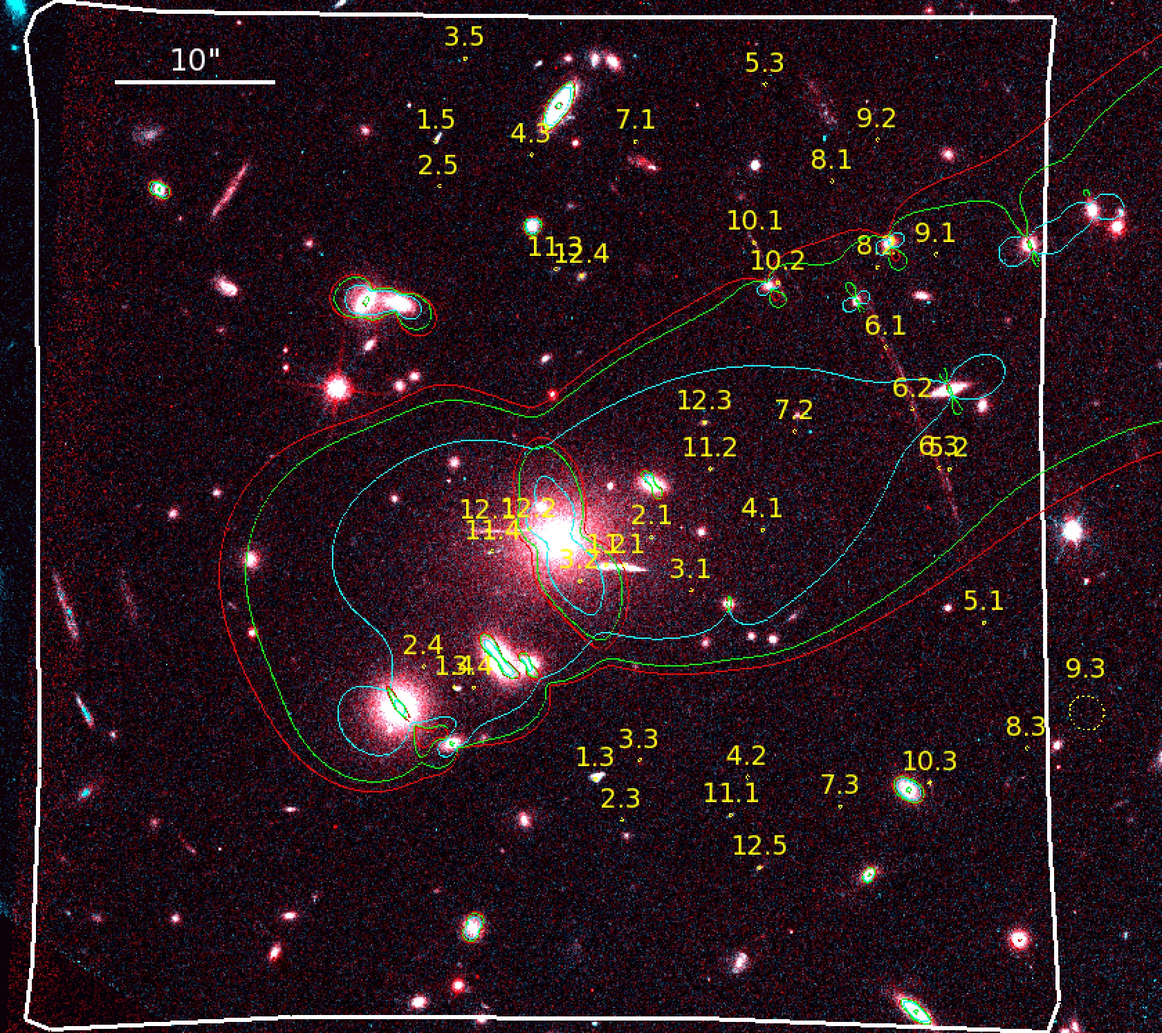
Figure 1: Overview of all multiple-image systems (in yellow) identified over a Hubble color image combining the F606W and F814W bands (north up, east left). The white polygon delineates the 1x1 arcmin² region covered by the MUSE observations used in this paper. The cyan, green and red lines show the critical lines predicted by our revised mass model (Sect. 4) at $z=1.46$ (system 6), $z=3.5077$ (systems 1 and 2) and $z=6.4085$ (system 9).

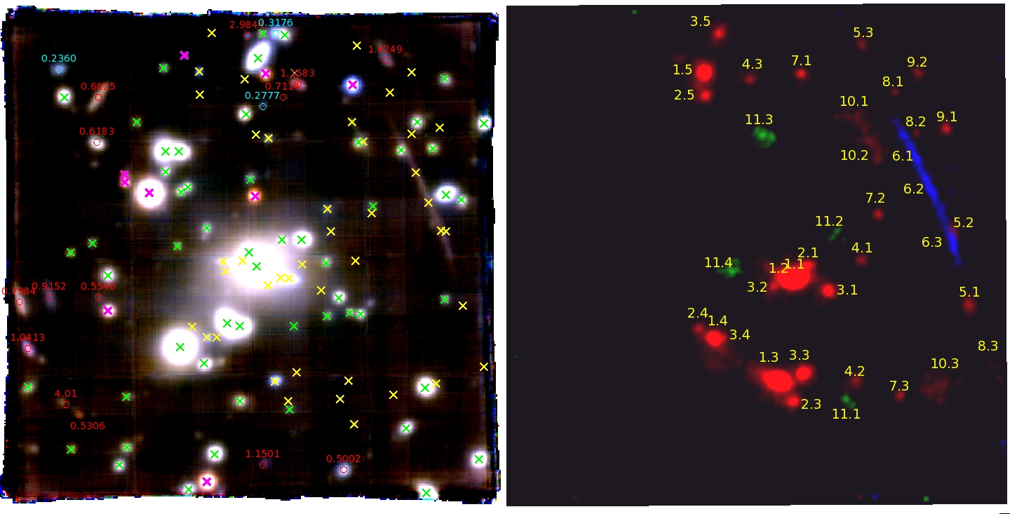
Figure 2: Overview of all redshifts measured in MUSE observations. The left panel shows a MUSE color image produced by collapsing three contiguous wavelength ranges in the whole cube. The green crosses identify cluster members confirmed by our spectroscopy. Cyan and red circles show the redshifts of foreground and single image background sources, respectively, while the yellow crosses mark the location of multiple images. The right panel shows a combination of all narrow band images showing the emission lines in multiply imaged systems 1 to 12. Lyman-$\alpha$ emitters are presented in red, while [OII] and CIII] emitters are shown in blue and green, respectively.

3 Data Analysis

We searched the MUSE datacube for spectral features, both for continuum-detected sources and for objects dominated by nebular emission lines. We first produced “white-light” and color images by collapsing the cube over its full wavelength range or in the blue/green/red wavelengths (Fig. 2, left panel). We ran SExtractor (Bertin & Arnouts, 1996) to identify objects in the white-light image and measured their continuum levels at 3 wavelengths. The spectra of these continuum sources were extracted using the spatial extent measured in the white light image.

In addition, we produced pseudo narrow-band images by performing a running average of 5 adjacent wavelength planes (6.25Å width) in the whole cube, using a weighting scheme to enhance the detection of typical $\sigma\sim 100$ km/s emission lines. We ran SExtractor again in each of these narrow-band images, and compared the detections with the previous continuum measurements to identify emission lines associated with continuum sources and isolated emission lines. Examples of continuum-subtracted narrow-band detections are given in Fig. 2 (right panel). All emission lines are well-detected and resolved over multiple wavelength planes throughout the cube.

Redshifts were measured for both continuum and emission-line dominated sources by identifying a combination of emission and absorption line features. The large majority of continuum sources identified are formed by cluster members (53) and foreground sources (3), easily recognisable with K 3933 Å and H 3969 Å absorption features (green and cyan crosses respectively in the left panel of Fig. 2). Background sources are all identified through their emission lines or Lyman-$\alpha$ break, in particular [OIII] 5007 Å at $z<0.8$, [OII] 3727 Å at $<1.5$, but for the large majority with Lyman-$\alpha$ 1216 Å at $z>2.8$ (Table 3). As Lyman-$\alpha$ is usually the only spectral feature visible in the MUSE wavelength range, we rely on its typical asymmetric shape and the absence of a doublet or other emission lines to ascertain the redshift (Fig. 3). We also measured the redshifts of candidate arcs and multiple images visible in HST images, through [OII] at $z=1.46$ (system 6), CIII] 1907,1909 Å at $z=2.2556$ (system 11) or a Lyman-$\alpha$ break at $z=3.41$ (system 12).

We searched through the redshifts measured in the cube for multiple images based on a preliminary mass modelling of the cluster core, which used only the 5-imaged system at $z=3.5077$ (Christensen et al., 2012). We found reliable connections for 43 sources forming a total of 12 systems (combining continuum and emission-line dominated sources), with the predictions from the model always lying within 1 arcsec from the detection. We then compared the extracted spectra for all 12 multiple images and found a very good match, as seen in Fig. 3. Together with our improved mass model (see Sect. 4) this clearly confirms these sources as multiple systems.

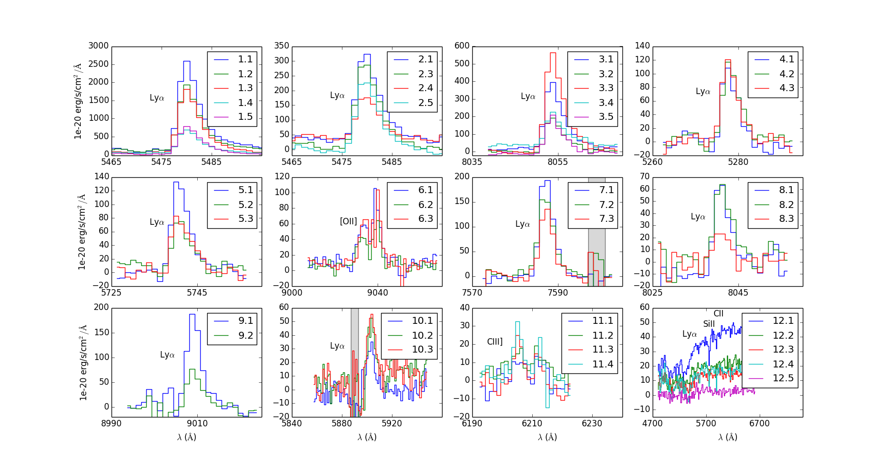
Figure 3: Extracted spectra of the strongest emission line in all identified multiple images, grouped by lensing system (in reading order). One can clearly see the asymmetric profile of all Lyman-$\alpha$ emission lines, as well as the doublet for [OII] and CIII]. In system 12 the main feature is the Lyman-$\alpha$ break as well as rest-frame UV absorption lines (SiII 1304 Å , CII 1334 Å). The grey areas mark the location of strong sky line residuals.

ID	$\alpha$ (hrs)	$\delta$ (deg)	$z_{\rm spec}$	$\mu$	line	flux
	20:31:	-40:37:				10-18 erg/s/cm2
1.1	52.90	32.5	3.508	$19.9\pm 1.9$	Ly$\alpha$	$185\pm 5$
1.2	52.99	32.5	3.508	$11.7\pm 1.2$	Ly$\alpha$	$169\pm 4$
1.3	53.05	45.8	3.508	$6.8\pm 0.2$	Ly$\alpha$	$270\pm 3$
1.4	53.83	40.1	3.508	$2.5\pm 0.1$	Ly$\alpha$	$42\pm 0.6$
1.5	53.93	06.0	3.508	$3.5\pm 0.1$	Ly$\alpha$	$110\pm 2$
2.1	52.74	30.7	3.508	$4.7\pm 0.2$	Ly$\alpha$	$22.4\pm 0.6$
2.2	[53.12]	[31.1]
2.3	52.91	48.4	3.508	$4.7\pm 0.1$	Ly$\alpha$	$21.1\pm 0.8$
2.4	53.99	38.8	3.508	$2.7\pm 0.1$	Ly$\alpha$	$10.4\pm 0.6$
2.5	53.90	08.9	3.508	$3.9\pm 0.1$	Ly$\alpha$	$16.4\pm 0.7$
3.1	52.53	34.1	5.623	$5.3\pm 0.2$	Ly$\alpha$	$37.6\pm 1.4$
3.2	53.14	33.5	5.623	$2.6\pm 0.1$	Ly$\alpha$	$17.7\pm 1.1$
3.3	52.81	44.6	5.623	$8.2\pm 0.3$	Ly$\alpha$	$56.6\pm 1.8$
3.4	53.72	40.1	5.623	$2.2\pm 0.1$	Ly$\alpha$	$11.6\pm 0.9$
3.5	53.76	00.9	5.623	$3.3\pm 0.1$	Ly$\alpha$	$24.8\pm 1.4$
4.1	52.14	30.3	3.340	$4.1\pm 0.1$	Ly$\alpha$	$8.3\pm 0.7$
4.2	52.22	45.7	3.340	$5.0\pm 0.1$	Ly$\alpha$	$12.6\pm 1.0$
4.3	53.40	06.9	3.340	$5.2\pm 0.1$	Ly$\alpha$	$9.9\pm 0.8$
5.1	50.92	36.1	3.723	$9.1\pm 0.2$	Ly$\alpha$	$14.3\pm 1.0$
5.2	51.11	26.5	3.723	$18.1\pm 0.8$	Ly$\alpha$	$6.8\pm 0.7$
5.3	52.12	02.5	3.723	$5.1\pm 0.1$	Ly$\alpha$	$6.5\pm 0.7$
6.1	51.46	18.9	1.425	$19.5\pm 1.0$	[OII]	$582\pm 13$
6.2	51.31	22.8	1.425	$11.8\pm 0.5$	[OII]	$578\pm 12$
6.3	51.17	26.4	1.425	$18.2\pm 0.6$	[OII]	$553\pm 11$
7.1	52.83	06.1	5.240	$4.9\pm 0.1$	Ly$\alpha$	$14.5\pm 0.8$
7.2	51.96	24.2	5.240	$4.2\pm 0.1$	Ly$\alpha$	$8.1\pm 0.6$
7.3	51.71	47.6	5.240	$4.1\pm 0.1$	Ly$\alpha$	$6.7\pm 0.5$
8.1	51.75	08.6	5.613	$15.0\pm 0.5$	Ly$\alpha$	$3.4\pm 0.4$
8.2	51.51	13.9	5.613	$14.0\pm 0.6$	Ly$\alpha$	$2.7\pm 0.3$
8.3	50.69	43.9	5.613	$4.1\pm 0.1$	Ly$\alpha$	$0.4\pm 0.1$
9.1	51.19	13.1	6.408	$14.8\pm 0.9$	Ly$\alpha$	$10.3\pm 0.8$
9.2	51.51	06.0	6.408	$13.8\pm 0.6$	Ly$\alpha$	$5.5\pm 0.7$
9.3	[50.36]	[41.7]
10.1	52.18	12.4	3.856	$14.1\pm 0.4$	Ly$\alpha$	$4.0\pm 0.8$
10.2	52.05	14.9	3.856	$4.1\pm 0.1$	Ly$\alpha$	$9.6\pm 1.3$
10.3	51.22	46.1	3.856	$6.1\pm 0.2$	Ly$\alpha$	$8.9\pm 1.3$
11.1	52.31	48.1	2.256	$3.7\pm 0.1$	CIII]	$2.5\pm 0.8$
11.2	52.42	26.5	2.256	$3.4\pm 0.1$	CIII]	$1.4\pm 0.6$
11.3	53.27	14.0	2.256	$5.6\pm 0.1$	CIII]	$9.6\pm 2.6$
11.4	53.62	31.6	2.256	$4.9\pm 0.3$	CIII]	$6.3\pm 1.4$
11.5	[53.27]	[30.8]
12.1	53.64	30.3	3.414	$5.6\pm 0.4$	Ly$\alpha$b
12.2	53.42	30.2	3.414	$4.3\pm 0.3$	Ly$\alpha$b
12.3	52.45	23.6	3.414	$4.4\pm 0.1$	Ly$\alpha$b
12.4	53.13	14.4	3.414	$7.3\pm 0.2$	Ly$\alpha$b
12.5	52.15	51.4	3.414	$3.2\pm 0.1$	Ly$\alpha$b

s1 & 55.37 49.2 4.010 $3.5\pm 0.1$ Ly$\alpha$ $12.8\pm 1.1$ s2 53.37 01.2 2.984 $3.4\pm 0.1$ Ly$\alpha$ $38.7\pm 1.5$ s3 51.80 04.1 1.425 $4.2\pm 0.2$ [OII] $75.6\pm 2.3$ s4 52.79 07.4 1.158 $3.1\pm 0.1$ [OII] $60.2\pm 2.0$ s5 53.16 56.3 1.150 $2.1\pm 0.1$ [OII] $19.1\pm 1.7$ s6 55.85 41.7 1.041 $2.3\pm 0.1$ [OII] $48.7\pm 1.7$ s7 55.61 35.0 0.9152 $2.5\pm 0.1$ [OII] $62.7\pm 1.4$ s8 55.94 35.6 0.7984 $2.0\pm 0.1$ [OII] $100.7\pm 1.3$ s9 52.97 09.0 0.7114 $2.2\pm 0.1$ [OII] $3.9\pm 0.8$ s10 55.06 09.2 0.6825 $1.7\pm 0.1$ [OII] $75.7\pm 1.9$ s11 55.07 15.2 0.6183 $1.8\pm 0.1$ [OII] $47.8\pm 1.9$ s12 55.05 35.0 0.5546 $1.4\pm 0.1$ [OII] $4.2\pm 1.0$ s13 55.27 50.1 0.5306 $1.9\pm 0.1$ K,H s14 52.28 57.2 0.5002 $1.4\pm 0.1$ [OII] $112.8\pm 3.9$

Table 1: Multiple image systems (top part) and other single image lensed sources (bottom part). From left to right we give their positions (J2000.0), measured redshifts, magnifications, main line feature detected and corresponding line flux. Ly$\alpha$b refers to the Lyman-$\alpha$ absorption break. Positions marked with brackets are not detected with MUSE but are predicted by the lens model (see text for details).

4 Cluster mass modelling

Following our previous work on cluster mass modelling (Limousin et al., 2007; Jauzac et al., 2014a), we used the locations and redshifts of the 12 multiple systems identified to constrain a parametric mass model of the cluster using the Lenstool (Jullo et al., 2007) software. In short, we adopt a dual pseudo-isothermal elliptical mass distribution (dPIE, also known as truncated PIEMD, see Elíasdóttir et al. 2007), which corresponds to an isothermal profile with two characteristic radii: a core radius r_core (producing a flattening of the mass distribution at the centre), and a cut radius r_cut (producing a drop-off of the mass distribution on large scales). Our preliminary mass model of SMACSJ2031, which we used in Christensen et al. (2012) to derive magnification factors, assumed a single cluster-scale dPIE component centred on the SE cluster as well as individual galaxy-scale dPIE profiles on each cluster member following a scaling relation with luminosity (see e.g. Richard et al. 2010).

With the addition of new multiple images, we refine this mass model by incorporating a second cluster-scale mass component centred on the NW cluster, located 1.2 arcmin away. This extends the critical line in the NW-SE direction (Fig. 1) and gives a much better match with the new systems 6 to 10 located in this region. One can clearly see the effect of this extension of the critical line towards the upper-right corner of the MUSE field-of-view, with an absence of multiple images identified in the lower-left corner. The best fit parameters of the new mass model are presented in Table 3.

Table 2: Best-fit model parameters of the cluster-scale dPIE profiles (SE and NW subclusters) and the scaling relation of cluster members (shown for a L^∗ galaxy. From left to right: center in arcsecs from the origin fixed at the location of the brightest cluster galaxy ($\alpha$=20:35:11.835,$\delta$=-40:27:08.47), ellipticity and position angle, core and cut radii, central velocity dispersion. Values in brackets are fixed in the modelling.

The two-component mass model now reproduces all 12 multiple systems with an rms of 0.41” in the image plane. Although the centroid precision of the emission lines is much better than this for the MUSE data (typically 0.1”) such a scatter is expected because of additional lensing structures along the line of sight (see the discussion in Jullo et al. 2010). An illustration of the ability to reproduce the systems is shown in the critical lines presented in Fig. 1 as we expect a symmetry of multiple images against the corresponding critical line. The projected cluster mass profile (radially integrated from the location of the brightest galaxy in the SE cluster) is presented in Fig. 4, together with the strong lensing constraints. We can see that the profile is best constrained within 10-150 kpc by the large number of multiple images. The precision obtained on the integrated mass in this region is a few percent, about 5 times better than the previous model.

We use this mass model to estimate the magnifications for all background sources, and report the values in Table 3. Errors on the magnification factors are estimated for each source by producing 500 mass models sampling the posterior probability distribution of the dPIE parameters, and measuring the distribution of magnifications at this location. Thanks to the high density of constraints in the cluster core, the relative error on magnification factors are typically $5-30\%$, which is similar to the precision reached in the Hubble Frontier Fields (Jauzac et al., 2014a).

We also check that all of the 14 other background sources identified (s1 to s14 in Table 3, ranging from $z=0.5$ to $z=4.01$) are indeed predicted to be single images by this model, as they are all located in the SE corner of the MUSE field-of-view. Three counter images identified are not detected in the observations for the following reasons: image 9.3 is predicted to lie outside of the MUSE field of view, and images 2.2 and 11.5 are predicted to be located under the brightest cluster member, thus suffering from strong cluster light contamination.

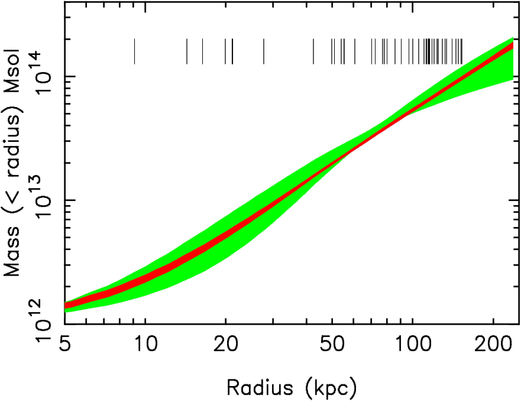
Figure 4: Projected cluster mass profile integrated over the radial distances from the center of the SE cluster (red curve). The radial distance of all multiple images used as strong-lensing constraints are marked with black ticks. We overplot in green the range of mass profiles allowed by the previous mass model (which only used constraints from system 1), showing the gain in precision obtained with the MUSE data.

To summarise, the sensitivity, resolution and wide field-of-view of MUSE, when coupled with the strong lensing region of a cluster core, form the perfect combination to detect numerous lensing systems and use them as constraints to measure the cluster mass profile. Further, more detailed analysis could include the resolved constraints from cluster members in the cluster core, for which we can measure the individual velocity dispersions with the MUSE data.

In addition, accounting for the magnification factor, we show here that we can reliably measure the redshifts for Lyman-$\alpha$ emitters that are intrinsically as faint as $2\times 10^{-19}$ erg/s/cm² (images 8.1 and 8.2) and up to $z=6.4$ (system 9). The multiplicity of these sources in the strong lensing regime helps to confirm these faint lines to be Lyman-$\alpha$. We expect that targeting lensing cluster with MUSE will result in the detection of a large number of such faint emitters at high redshift.

Acknowledgments

We thank Eric Emsellem for his comments on the manuscript. JR and VP acknowledges support from the ERC starting grant CALENDS. JR acknowledges support from the CIG grant 294074. Based on observations made with ESO Telescopes at the La Silla Paranal Observatory under programme ID 60.A-9100(B). We thank all the staff at Paranal Observatory for their valuable support during the commissioning of MUSE. Also based on observations made with the NASA/ESA Hubble Space Telescope (PID 12166 and 12884).

References

- Bacon et al. (2010) Bacon R. e. al., 2010, in Society of Photo-Optical Instrumentation Engineers (SPIE) Conference Series Vol. 7735 of Society of Photo-Optical Instrumentation Engineers (SPIE) Conference Series
- Bertin & Arnouts (1996) Bertin E., Arnouts S., 1996, Astronomy & Astrophysics Supplement, 117, 393
- Christensen et al. (2012) Christensen L., Richard J., Hjorth J., Milvang-Jensen B., Laursen P., Limousin M., Dessauges-Zavadsky M., Grillo C., Ebeling H., 2012, MNRAS, 427, 1953
- Ebeling et al. (2001) Ebeling H., Edge A. C., Henry J. P., 2001, ApJ, 553, 668
- Ebeling et al. (2010) Ebeling H., Edge A. C., Mantz A., Barrett E., Henry J. P., Ma C. J., van Speybroeck L., 2010, MNRAS, 407, 83
- Elíasdóttir et al. (2007) Elíasdóttir Á., Limousin M., Richard J., Hjorth J., Kneib J.-P., Natarajan P., Pedersen K., Jullo E., Paraficz D., 2007, astro-ph/0710.5636
- Grillo & et al. (2014) Grillo C., et al. 2014, submitted, arXiv/1407.7866
- Jauzac et al. (2014a) Jauzac M., Clément B., Limousin M., Richard J., Jullo E., Ebeling H., Atek H., Kneib J.-P., Knowles K., Natarajan P., Eckert D., Egami E., Massey R., Rexroth M., 2014, MNRAS, 443, 1549
- Jauzac et al. (2014b) Jauzac M., Jullo E., Eckert D., Ebeling H., Richard J., Limousin M., Atek H., Kneib J.-P., Clément B., Egami E., Harvey D., Knowles K., Massey R., Natarajan P., Rexroth M., 2014, submitted to MNRAS, astro-ph/1406.3011
- Johnson et al. (2014) Johnson T. L., Sharon K., Bayliss M. B., Gladders M. D., Coe D., Ebeling H., 2014, ApJ submitted, arXiv:1405.0222
- Jullo et al. (2007) Jullo E., Kneib J.-P., Limousin M., Elíasdóttir Á., Marshall P. J., Verdugo T., 2007, New Journal of Physics, 9, 447
- Jullo et al. (2010) Jullo E., Natarajan P., Kneib J.-P., D’Aloisio A., Limousin M., Richard J., Schimd C., 2010, Science, 329, 924
- Kneib & Natarajan (2011) Kneib J.-P., Natarajan P., 2011, A&A Rev., 19, 47
- Koekemoer et al. (2002) Koekemoer A. M., Fruchter A. S., Hook R. N., Hack W., 2002, in S. Arribas, A. Koekemoer, & B. Whitmore ed., The 2002 HST Calibration Workshop pp 337–+
- Limousin et al. (2012) Limousin M., Ebeling H., Richard J., Swinbank A. M., Smith G. P., Jauzac M., Rodionov S., Ma C.-J., Smail I., Edge A. C., Jullo E., Kneib J.-P., 2012, A&A, 544, A71
- Limousin et al. (2007) Limousin M., Richard J., Jullo E., Kneib J.-P., Fort B., Soucail G., Elíasdóttir Á., Natarajan P., Ellis R. S., Smail I., Czoske O., Smith G. P., Hudelot P., Bardeau S., Ebeling H., Egami E., Knudsen K. K., 2007, ApJ, 668, 643
- Richard et al. (2014) Richard J., Jauzac M., Limousin M., Jullo E., Clément B., Ebeling H., Kneib J.-P., Atek H., Natarajan P., Egami E., Livermore R., Bower R., 2014, MNRAS, 444, 268
- Richard et al. (2009) Richard J., Pei L., Limousin M., Jullo E., Kneib J. P., 2009, A&A, 498, 37
- Richard et al. (2010) Richard J., Smith G. P., Kneib J.-P., Ellis R. S., Sanderson A. J. R., Pei L., Targett T. A., Sand D. J., Swinbank A. M., Dannerbauer H., Mazzotta P., Limousin M., Egami E., Jullo E., Hamilton-Morris V., Moran S. M., 2010, MNRAS, 404, 325
- Zitrin et al. (2011) Zitrin A., Broadhurst T., Barkana R., Rephaeli Y., Benítez N., 2011, MNRAS, 410, 1939
- Zitrin et al. (2012) Zitrin A., Rosati P., Nonino M., Grillo C., Postman M., Coe D., Seitz S., Eichner T., Broadhurst T., Jouvel S., Balestra I., Mercurio A., Scodeggio M., Benítez N., Bradley L., 2012, ApJ, 749, 97