Improving the Precision of Weak Measurements by Postselection Measurement

Abstract

Postselected weak measurement is a useful protocol for amplifying weak physical effects. However, there has recently been controversy over whether it gives any advantage in precision. While it is now clear that retaining failed postselections can yield more Fisher information than discarding them, the advantage of postselection measurement itself still remains to be clarified. In this Letter, we address this problem by studying two widely used estimation strategies: averaging measurement results, and maximum likelihood estimation, respectively. For the first strategy, we find a surprising result that squeezed coherent states of the pointer can give postselected weak measurements a higher signal-to-noise ratio than standard ones while all standard coherent states cannot, which suggests that raising the precision of weak measurements by postselection calls for the presence of “nonclassicality” in the pointer states. For the second strategy, we show that the quantum Fisher information of postselected weak measurements is generally larger than that of standard weak measurements, even without using the failed postselection events, but the gap can be closed with a proper choice of system state.

Introduction.— Postselected weak measurement is a quantum measurement protocol first invented by Aharonov, Albert, and Vaidman in 1988 Aharonov et al. (1988). It involves weak coupling between the system and the pointer, but the postselection on the system leads to a surprisingly counterintuitive effect: the average shift of the final pointer state can go far beyond the eigenvalue spectrum of the system observable (multiplied by the coupling constant) in sharp contrast to the projective quantum measurement. The mechanism behind this effect is the coherence between the pointer states translated by different eigenvalues of the system observable, which has an enlightening interpretation based on superoscillation Berry and Shukla (2012).

Postselected weak measurement has aroused enormous research interest in different fields, due to its ability to amplify tiny physical effects. Thanks to technical progress in recent years, the weak value has been measured in experiments Ritchie et al. (1991); Pryde et al. (2005); Groen et al. (2013); Campagne-Ibarcq et al. (2014), and postselected weak measurements have been applied to measuring small parameters in various systems, including optical systems Hosten and Kwiat (2008); Dixon et al. (2009); Starling et al. (2009, 2010a, 2010b); Pfeifer and Fischer (2011); Turner et al. (2011); Egan and Stone (2012); Gorodetski et al. (2012); Hofmann et al. (2012); Zhou et al. (2012); Viza et al. (2013); Xu et al. (2013); Goswami et al. (2014); Magaña Loaiza et al. (2014); Mirhosseini et al. (2014); Viza et al. (2015), atomic systems Shomroni et al. (2013) and NMR Lu et al. (2014). More experimental protocols have also been proposed Brunner and Simon (2010); Feizpour et al. (2011); Li et al. (2011); Zilberberg et al. (2011); Götte and Dennis (2012); Nishizawa et al. (2012); Wu and Żukowski (2012); Dressel et al. (2013); Hayat et al. (2013); Strübi and Bruder (2013); Zhou et al. (2013); Huang and Agarwal (2015); Lyons et al. (2015). A general framework for postselected weak measurement is given in Wu and Li (2011), and reviews of the field can be found in Shikano (2012); Kofman et al. (2012); Dressel et al. (2014). Of course, weak value amplification cannot be arbitrarily large in practice. The condition for the validity of the weak value formalism was discussed in Duck et al. (1989), and the limit of amplification has been studied in Koike and Tanaka (2011); Susa et al. (2012); Di Lorenzo (2014); Pang et al. (2014a).

One of the major goals in postselected weak measurement is to enhance the sensitivity of estimating small parameters. The experiment of Starling et al. Starling et al. (2009) and the proposal of Feizpour et al. Feizpour et al. (2011) showed that postselection can significantly raise the signal-to-noise ratio (SNR) of weak measurement. Nevertheless, some other work has led to a negative conclusion Knee et al. (2013). In recent research, it was shown that the failed postselections contain Fisher information Tanaka and Yamamoto (2013); Ferrie and Combes (2014); Zhang et al. (2015), and even the distribution probabilities of postselection results can carry Fisher information Zhang et al. (2015); thus, discarding postselection results will generally lead to a loss of precision Combes et al. (2014).

To address the issue of low postselection efficiency, Dressel et al. Dressel et al. (2013) and Lyons et al. Lyons et al. (2015) proposed recycling the unpostselected photons to improve the precision. It was later found Jordan et al. (2014); Pang et al. (2014b); Pang and Brun (2015) that the successful postselections can concentrate most of the Fisher information in the pointer, and the Fisher information of postselected weak measurement can approximately reach the Heisenberg limit Jordan et al. (2014); Pang et al. (2014b); Jordan et al. (2015); Zhang et al. (2015); Pang and Brun (2015). More surprising, weak value amplification can improve the precision in the presence of technical noise Feizpour et al. (2011); Jordan et al. (2014); Pang and Brun (2015), and technical noise may increase the SNR of postselected weak measurement Kedem (2012). A review of the controversy over the advantage of weak value amplification is given in Knee et al. (2014).

The postselection in a weak measurement includes two steps: first, measure the system, second, postselect the measurement results. Most previous research focused on whether failed postselections should be retained or not, provided the system is measured. However, a more fundamental problem is whether the system should be measured at all in order to enhance the precision of weak measurement. If the measurement on the system could not give any advantage, then it would become meaningless to study whether the failed postselections should be used or not. So, this question lies at the heart of postselected weak measurement: what is the significance of measuring the system in a weak measurement compared to the standard weak measurement (i.e., without measuring the system)? Since postselecting and nonpostselecting the results of measuring the system only lead to a negligible difference in the Fisher information Pang et al. (2014b); Pang and Brun (2015), we will focus only on comparing postselected weak measurement to the standard weak measurement.

At first glance, this question seems easy to answer: since measuring the system with proper postselection can amplify the signal, the SNR can then also be increased. However, the efficiency of postselection is rather low, which may cancel the benefits of the amplification effect in the SNR, so the problem becomes subtle. In fact, the numerical results in Zhu et al. (2011) showed that postselecting the system with Gaussian pointer states cannot improve the SNR compared with standard weak measurements, and Knee and Gauger (2014) found similar results for the Fisher information of measuring the position or momentum of the pointer, with the pointer states being real or Gaussian and the weak values being real or imaginary, respectively.

However, it is important to note that those studies did not optimize over the choice of the system and pointer states, so they do not rule out the existence of other choices that may allow postselected weak measurements to have higher precision. In particular, the Gaussian states considered heretofore are quite “classical,” so it is of great interest whether using more “quantum” states can bring any advantage for precision. In fact, it has been shown that nonclassical quantum states can be favorable to some other weak measurement protocols, e.g., consecutive violations of Clauser-Horne-Shimony-Holt (CHSH) inequalities Silva et al. (2015). Moreover, the measurement basis of the pointer was not optimized either; hence it is also possible to have the Fisher information increased by measurements other than those along the basis of position or momentum of the pointer.

Answering these questions will clarify the advantage of postselection in weak measurements, and it is exactly the aim of this Letter. We study the optimal precision of both postselected and standard weak measurements for general system and pointer states, and investigate when or whether postselected weak measurements can have higher precision than standard weak measurements. Moreover, different estimation strategies may also influence the precision, so we consider two principal estimation strategies: averaging the measurement results of the pointer (AMR), and maximum likelihood estimation (MLE), both of which have been widely used in practice.

For the strategy of AMR, an interesting result we find is that all standard (i.e., unsqueezed) coherent states do not give weak measurements an improvement in SNR with postselection, but properly squeezed coherent states do. This suggests that, for weak value amplification to enhance the precision, a necessary ingredient is some nonclassicality in the initial pointer states which was missing from previous studies. This result extends the understanding and feasibility of postselected weak measurement in parameter estimation.

For the strategy of MLE, we obtain the optimum quantum Fisher information and show that, even without using the failed postselections, the quantum Fisher information of postselected weak measurements is generally higher than that of standard weak measurements.

Weak value formalism.— First, we review the weak value formalism for postselected weak measurement. Suppose the initial state of the system is $|\Psi_{i}\rangle$ and the initial state of the pointer is $|D\rangle$. The interaction Hamiltonian between the system and the pointer is

$$H_{\mathrm{int}}=gA\otimes\Omega\delta(t-t_{0}),$$ (1)

where the $\delta$ function indicates that the interaction is instantaneous at time $t_{0}$. Let $\hbar=1$. After the interaction (1), the system is postselected to $|\Phi_{f}\rangle$, then the state of the pointer collapses to $|D_{f}\rangle=\langle\Phi_{f}|\exp(-\mathrm{i}gA\otimes\Omega)|\Phi_{i}\rangle|D\rangle$ (unnormalized). It can be derived that $|D_{f}\rangle\approx\langle\Phi_{f}|\Phi_{i}\rangle(1-\mathrm{i}gA_{w}\Omega)|D\rangle$ when $gA_{w}\ll 1$, where $A_{w}$ is the weak value, defined as

$$A_{w}=\frac{\langle\Phi_{f}|A|\Phi_{i}\rangle}{\langle\Phi_{f}|\Phi_{i}\rangle}.$$ (2)

If one measures an observable $M$ on the pointer state $|D_{f}\rangle$, it can be obtained sup that the average shift is

$$\langle\Delta M\rangle_{f} \approx g\mathrm{Im}A_{w}(\langle\{\Omega,M\}\rangle_{D}-2\langle\Omega\rangle_{D}\langle M\rangle_{D})$$ (3)

$$+\mathrm{i}g\mathrm{Re}A_{w}\langle[\Omega,M]\rangle_{D},$$

where $\langle D|\cdot|D\rangle$ is denoted as $\langle\cdot\rangle_{D}$ for short. And the success probability of postselection is $P_{s}\approx|\langle\Phi_{f}|\Phi_{i}\rangle|^{2}.$

The weak value (2) can be very large when $\langle\Phi_{f}|\Phi_{i}\rangle\ll 1$, and the dependence of $\langle\Delta M\rangle_{f}$ on $A_{w}$ in Eq. (3) indicates that the average shift can go beyond any eigenvalue of $A$ in this case. This is the origin of the weak value amplification.

Optimal signal-to-noise ratio.— First, we study the precision of postselected weak measurement, then compare it with that of standard weak measurement, to determine when or whether postselection can assist weak measurement in precision.

To quantify the precision of estimating the parameter $g$, a widely used benchmark is the signal-to-noise ratio of the estimates, defined as

$$\mathrm{SNR}_{{\rm post}}=\frac{\sqrt{NP_{s}}\langle\Delta M\rangle_{f}}{\sqrt{\mathrm{Var}(M)_{{}_{f}}}},$$ (4)

where $N$ is the total number of measurements. The factor $\sqrt{P_{s}}$, due to $\mathrm{Var}(M)_{{}_{f}}$, scales inversely with the number of successful postselections. In the first order approximation with respect to $g$, the spread of the pointer wave function is almost unchanged, so $\mathrm{Var}(M)_{{}_{f}}\approx\mathrm{Var}(M)_{D}.$

Note that the quantity defined in Eq. (4) is the SNR of the AMR estimator, not of the measurement results, and it is directly related to the estimation precision of postselected weak measurement sup .

With different pre- and postselections of the system, the SNR is usually different, so a proper measure for the precision of postselected weak measurement is the maximum SNR over all possible pre- and postselections. Direct maximization of the SNR by usual means (such as the variation method) is rather difficult, since the variation of $\mathrm{SNR}_{{\rm post}}$ (4) produces a nonlinear equation that is not easy to deal with.

However, the results of Pang et al. (2014b) offer an alternative possible approach to this hard problem. In that Letter, the largest success probability over all postselections of the system for a given weak value $A_{w}$ was shown to be

$$\max_{|\Phi_{f}\rangle}P_{s}\approx\frac{\mathrm{Var}(A)_{i}}{\langle A^{2}\rangle_{i}-2\langle A\rangle_{i}\mathrm{Re}A_{w}+|A_{w}|^{2}},$$ (5)

where $\langle\cdot\rangle_{i}$ is short for $\langle\Phi_{i}|\cdot|\Phi_{i}\rangle$. By exploiting this result, the task of maximizing the SNR over all pre- and postselections can be simplified to maximizing over all weak values $A_{w}$.

Usually the weak value $A_{w}$ is complex, and can be denoted as $A_{w}=|A_{w}|\mathrm{e}^{\mathrm{i}\theta}$, so we can follow a two-step procedure to obtain the maximum of the $\mathrm{SNR}_{{\rm post}}$ over $A_{w}$: first, maximize $\mathrm{SNR}_{{\rm post}}$ over $|A_{w}|$, then maximize it over $\theta$.

The mathematical detail of this optimization is left for the Supplemental Material. The result of the maximized $\mathrm{SNR}_{{\rm post}}$ turns out to be

$$g\eta(\varphi)\sqrt{N\frac{(\langle\{\Omega,M\}\rangle_{D}-2\langle\Omega\rangle_{D}\langle M\rangle_{D})^{2}+|\langle[\Omega,M]\rangle_{D}|^{2}}{\mathrm{Var}(M)_{D}}},$$ (6)

where $\varphi=\arctan\frac{\mathrm{i}\langle[\Omega,M]\rangle_{D}}{\langle\{\Omega,M\}\rangle_{D}-2\langle\Omega\rangle_{D}\langle M\rangle_{D}}$ and $\eta(\varphi)=\sqrt{\mathrm{Var}(A)_{i}+\langle A\rangle_{i}^{2}\sin^{2}\varphi}$.

In sup , we also obtained an upper bound on the optimal $\mathrm{SNR}_{{\rm post}}$ based on (6).

When can SNR be increased?— The maximum SNR (6) quantifies the metrological performance of postselected weak measurement. To address the question of when (or whether) postselection can improve the SNR of weak measurement, we need to further compare (6) with the maximum SNR of standard weak measurement.

Before proceeding with this question, it is helpful to note that in the average shift of the pointer (3), the real part of the weak value is assigned with the commutator between $\Omega,\,M$ and the imaginary part with the covariance between $\Omega,\,M$. These coefficients can be quite large with proper pointer states and will not be counterbalanced by the low postselection probability while the weak values may be. So it opens the possibility of increasing the SNR by postselection.

In a standard weak measurement, the average shift in the observable $M$ on the postinteraction pointer state is $\langle\Delta M\rangle=\mathrm{i}g\langle A\rangle_{i}\langle[\Omega,M]\rangle_{D}$ sup , and $\max\langle A\rangle_{i}=\lambda_{\max}(A)$, so the optimal SNR is

$$\max\mathrm{SNR}_{{\rm std}}=g\frac{\sqrt{N}|\lambda_{\max}(A)\langle[\Omega,M]\rangle_{D}|}{\sqrt{\mathrm{Var}(M)_{D}}}.$$ (7)

The ratio between the optimal SNR of postselected and standard weak measurements is, therefore,

$$s=\frac{\sqrt{\mathrm{Var}(A)_{i}\csc^{2}\varphi+\langle A\rangle_{i}^{2}}}{|\lambda_{\max}(A)|}.$$ (8)

Obviously, since $\csc^{2}\varphi\geq 1$, when $|\Phi_{i}\rangle\rightarrow|\lambda_{\max}(A)\rangle$, $\sqrt{\mathrm{Var}(A)_{i}\csc^{2}\varphi+\langle A\rangle_{i}^{2}}\geq|\lambda_{\max}(A)|$, and thus $s\geq 1,$ which means that postselection in weak measurement will not reduce the SNR at least, but this is still not enough. The key question is when (or whether) $\csc^{2}\varphi>1$ can hold, so that postselection gives an increase of the SNR compared with standard weak measurement.

To answer this question, we move to Fock space. Suppose that $\Omega=q,\,M=p$. Then $[\Omega,M]{}_{D}=\mathrm{i}.$ In Fock space, $q$ and $p$ can be represented by $q=(a+a^{\dagger})/\sqrt{2},\,p=(a-a^{\dagger})/\sqrt{2}\mathrm{i},$ so $\{q,p\}=\mathrm{i}(a^{\dagger 2}-a^{2}),$ and $\csc^{2}\varphi=1+\left|\langle a^{\dagger 2}\rangle+\langle a\rangle_{D}^{2}-\langle a^{\dagger}\rangle_{D}^{2}-\langle a^{2}\rangle_{D}\right|^{2}.$

When the initial pointer state $|D\rangle$ is a standard coherent state, $\csc^{2}\varphi=1$, so standard coherent states cannot give postselected weak measurements any advantage in SNR over standard weak measurements. This generalizes the results of Zhu et al. (2011); Knee and Gauger (2014), and suggests that “classical” pointer states are not able to improve the SNR of postselected weak measurements.

An interesting question is whether introducing “nonclassicality” to the pointer state can “activate” the advantage of postselected weak measurement in SNR. Consider squeezed coherent states for the pointer. Suppose the initial state $|D\rangle$ of the pointer is

$$|\xi,\alpha\rangle=\exp\frac{1}{2}(\xi^{*}a^{2}-\xi a^{\dagger 2})|\alpha\rangle,$$ (9)

where $\xi$ is the squeeze parameter. Let $\xi=r\mathrm{e}^{\mathrm{i}\theta}$, then one can find sup

$$\csc^{2}\varphi=1+4(\sin\theta\sinh r\cosh r)^{2}.$$ (10)

It is clear from (10) that when $\sin\theta\neq 0$, one can acquire $\csc^{2}\varphi>1$ with a large $r$, so according to (8), if $\mathrm{Var}(A)_{i}\neq 0$, the SNR of postselected weak measurements exceeds that of standard weak measurements in this case. This shows that nonclassicality really can assist the postselection to improve the SNR of weak measurements. It is in a similar spirit to Ref. Feizpour et al. (2011): correlations, classical or quantum, can increase the SNR of weak measurements.

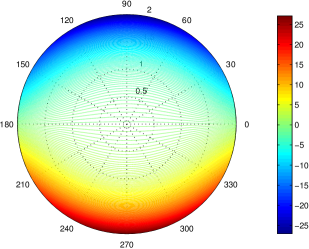
Figure 1: (Color online) The contours of $s$ are plotted for the squeezed vacuum states $|\xi,0\rangle=\exp\frac{1}{2}(\xi^{*}a^{2}-\xi a^{\dagger 2})|0\rangle$ with $|\xi|\leq 2$ and $|\arg\xi|\leq\pi$. The interaction Hamiltonian is $g\sigma_{z}\otimes q$ with $g=10^{-5}$. The weak value is fixed to $20\mathrm{i}$. The momentum $p$ is measured on the pointer after the postselection. Each point in the figure represents a $\xi$ on the complex plane, and the color indicates the corresponding value of $s$, which is the ratio between the SNR of postselected and standard weak measurements. It clearly shows $|s|$ can be much larger than $1$ with proper $\xi$, implying an increase in the SNR by postselecting the system. The sign of $s$ denotes the relative sign between the results of postselected and standard weak measurements.

To illustrate the above result, Fig. 1 plots the contours of the ratio $s$ on the complex plane of $\xi$ for the squeezed vacuum state $|\xi,0\rangle$. Improvement of SNR can be explicitly observed in the figure.

Why are squeezed coherent states more beneficial to the SNR than standard coherent states? It can be roughly understood from the following. The SNR of postselected weak measurement can be shown to be bounded by $\sqrt{\mathrm{Var}(\Omega)_{D}}$ sup , and the SNR of standard weak measurement is proportional to $1/\sqrt{\mathrm{Var}(M)_{D}}$ (see Eq. (7)). The ratio between them is approximately $\sqrt{\mathrm{Var}(\Omega)_{D}\mathrm{Var}(M)_{D}}$. Since coherent states have minimal uncertainty, $\sqrt{\mathrm{Var}(\Omega)_{D}\mathrm{Var}(M)_{D}}$ does not change and keeps the minimum for conjugate quadratures $\Omega$ and $M$. In contrast, squeezing can increase $\mathrm{Var}(\Omega)_{D}$ and decrease $\mathrm{Var}(M)_{D}$, so it can simultaneously increase the SNR of both types of weak measurements. However, squeezed coherent states no longer have the minimum uncertainty, so $\sqrt{\mathrm{Var}(\Omega)_{D}\mathrm{Var}(M)_{D}}$ can be increased. Hence, the SNR of postselected weak measurement can be raised more than that of standard weak measurement.

It is worth noting that squeezing may also simultaneously decrease $\mathrm{Var}(\Omega)_{D}$ and increase $\mathrm{Var}(M)_{D}$ instead, and the SNR of postselected weak measurement can still be higher than that of standard weak measurement. But in this case, the SNR of both types of weak measurements are decreased, so it should be avoided in practice.

Optimal quantum Fisher information.— Next, we turn to the precision of weak measurements using maximum likelihood estimation strategy. Once again, our goal is to determine whether postselected or standard weak measurement has greater precision, and what conditions determine the advantage.

The exact variance of the MLE estimator is usually difficult to obtain; however, Cramér and Rao Cramér (1946) showed that it is inversely bounded by the Fisher information, and this bound can be saturated in the asymptotic limit. So we will use Fisher information as the measure of precision for MLE instead.

As different measurements on the pointer produce different Fisher information, a proper benchmark for the precision of MLE is the maximum Fisher information over all possible measurements on the pointer, called the quantum Fisher information Braunstein and Caves (1994); Braunstein et al. (1996), and it gives a more general bound than that found by working in only one specific measurement basis. For a pure $g$-dependent state $|\psi_{g}\rangle$, the quantum Fisher information of estimating $g$ is $F^{(Q)}=4(\langle\partial_{g}\psi_{g}|\partial_{g}\psi_{g}\rangle-|\langle\psi_{g}|\partial_{g}\psi_{g}\rangle|^{2})$.

In a postselected weak measurement, the pointer state after postselecting the system is $|D_{f}\rangle\approx\mathrm{e}^{-\mathrm{i}gA_{w}\Omega}|D\rangle$, so $|\partial_{g}D_{f}\rangle\approx-(\mathrm{i}A_{w}\Omega+\langle\Omega\rangle_{D}\mathrm{Im}A_{w})|D\rangle$, and the quantum Fisher information is approximately sup

$$F_{{\rm post}}^{(Q)}\approx 4P_{s}|A_{w}|^{2}\mathrm{Var}(\Omega)_{D},$$ (11)

where we note the dependence on the postselection probability $P_{s}$. The maximum $P_{s}$ is given by (5), therefore, the maximum quantum Fisher information over all postselections given the weak value $A_{w}$ is

$$F_{{\rm post}}^{(Q)}\approx\frac{4|A_{w}|^{2}\mathrm{Var}(A)_{i}\mathrm{Var}(\Omega)_{D}}{\langle A^{2}\rangle_{i}-2\langle A\rangle_{i}\mathrm{Re}A_{w}+|A_{w}|^{2}}.$$ (12)

Now, the task is just to maximize $F_{{\rm post}}^{(Q)}$ over $A_{w}$. This maximization can be achieved by a two-step procedure similar to maximizing $\mathrm{SNR}_{{\rm post}}$ sup , and the result is

$$\max F_{{\rm post}}^{(Q)}\approx 4\langle A^{2}\rangle_{i}\mathrm{Var}(\Omega)_{D}.$$ (13)

As a comparison, consider the standard weak measurement. In this case, the postinteraction pointer state is generally a mixed state since the pointer is entangled with the system by the weak interaction. The quantum Fisher information for mixed states is much more complex than that for pure states, and a general analytical result is unavailable.

However, with the weak coupling limit $gA_{w}\ll 1$, this difficulty can be significantly reduced, since the postinteraction pointer state can be approximated to a pure state $|D_{f}\rangle\approx\mathrm{e}^{-\mathrm{i}g\langle A\rangle_{i}\Omega}|D\rangle$ sup . Then, one can immediately derive the quantum Fisher information for standard weak measurement

$$F_{{\rm std}}^{(Q)}\approx 4\langle A\rangle_{i}^{2}\mathrm{Var}(\Omega)_{D}.$$ (14)

Now, comparing $F_{{\rm std}}^{(Q)}$ with $F_{{\rm post}}^{(Q)}$, the ratio between them can be obtained:

$$\frac{F_{{\rm post}}^{(Q)}}{F_{{\rm std}}^{(Q)}}\approx\frac{\langle A^{2}\rangle_{i}}{\langle A\rangle_{i}^{2}}.$$ (15)

The result (15) compares the quantum Fisher information between postselected and standard weak measurements for every possible state of the system, in contrast to Ref. Knee and Gauger (2014); Knee et al. (2014) where the Fisher information of measuring the pointer along the position or momentum basis was compared between the two types of weak measurements for their respective optimal system states (with additional assumptions as reviewed in the Introduction). Eq. (15) indicates that the initial state of the system decides the ratio of quantum Fisher information, and implies the postselected weak measurement generally possesses more Fisher information than the standard weak measurement, except that the latter can catch up when the initial system is in an eigenstate of $A$.

Ref. Tanaka and Yamamoto (2013); Ferrie and Combes (2014); Zhang et al. (2015) made the comparison between using and discarding failed postselections, given that the system is measured. Ref. Jordan et al. (2014); Pang et al. (2014b); Pang and Brun (2015) showed that the difference between the Fisher information in these two cases can be shrunk to be negligibly small. Combining (15) with those results, if we denote the quantum Fisher information retaining all failed postselections as $F_{{\rm all}}^{(Q)}$, then

$$F_{{\rm all}}^{(Q)}\gtrsim F_{{\rm post}}^{(Q)}\geq F_{{\rm std}}^{(Q)}.$$ (16)

This clearly shows the relation of the quantum Fisher information between different types of weak measurements, and clarifies when the postselected weak measurement has metrological advantage. The first inequality of (16) reflects the results of Tanaka and Yamamoto (2013); Ferrie and Combes (2014); Jordan et al. (2014); Pang et al. (2014b); Zhang et al. (2015); Pang and Brun (2015), and the equality sign of the second inequality accords with Knee and Gauger (2014); Knee et al. (2014).

Remark.— The results for SNR and Fisher information at first glance seem quite different: a significant advantage can be given by postselected weak measurements over standard weak measurements in SNR, while the advantage is quite limited in Fisher information. The difference is rooted in the performances of the two estimators behind them, AMR and MLE, respectively. MLE has the minimum variance over all estimators, while AMR does not, and the Fisher information is usually an upper bound on the precision of MLE (except for Gaussian distributions) which can be achieved only asymptotically. Because of these differences, the SNR has more room to be improved than the Fisher information by optimizing the measurement strategy and the initial states of the system and pointer. These results indicate that the advantage of postselected weak measurements has dependence on the choice of estimation strategy.

This research was supported by the ARO MURI under Grant No. W911NF-11-1-0268.

Supplemental Material

I Average shift of the pointer

In this section, we show how to derive the average shift of the pointer for postselected weak measurements and standard weak measurements, respectively.

I.1 Postselected weak measurements

The interaction Hamiltonian between the system and the pointer is

$$H_{\mathrm{int}}=gA\otimes\Omega\delta(t-t_{0}).$$ (S1)

Suppose the initial state of the system is $|\Phi_{i}\rangle$, and the initial state of the pointer is $|D\rangle$. The system is postselected in the state $|\Phi_{f}\rangle$ after the interaction (S1), and the pointer collapses to the state (unnormalized)

$$|D_{f}\rangle=\langle\Phi_{f}|\exp(-\mathrm{i}gA\otimes\Omega)|\Phi_{i}\rangle|D\rangle.$$ (S2)

When $g$ is sufficiently small, $|D_{f}\rangle$ is approximately

$$|D_{f}\rangle \approx\langle\Phi_{f}|(1-\mathrm{i}gA\otimes\Omega)|\Phi_{i}\rangle|D\rangle$$ (S3)

$$=\langle\Psi_{f}|\Psi_{i}\rangle(1-\mathrm{i}gA_{w}\Omega)|D\rangle,$$

where $A_{w}$ is the so-called weak value, defined as $A_{w}=\frac{\langle\Psi_{f}|A|\Psi_{i}\rangle}{\langle\Psi_{f}|\Psi_{i}\rangle}.$ The success probability of postselection is

$$P_{s}\approx|\langle\Psi_{f}|\Psi_{i}\rangle|^{2}.$$ (S4)

The average shift in the measured value of the pointer observable $M$ is

$$\langle\Delta M\rangle_{f}=\frac{\langle D_{f}|M|D_{f}\rangle}{\langle D_{f}|D_{f}\rangle}-\langle M\rangle_{D}.$$ (S5)

We denote $\langle D|\cdot|D\rangle$ as $\langle\cdot\rangle_{D}$ for short throughout the paper. Note that

$$\langle D_{f}|M|D_{f}\rangle \approx|\langle\Psi_{f}|\Psi_{i}\rangle|^{2}(\langle M\rangle_{D}+\mathrm{i}g\mathrm{Re}A_{w}\langle[\Omega,M]\rangle_{D}+g\mathrm{Im}A_{w}\langle\{\Omega,M\}\rangle_{D}),$$ (S6)

$$\langle D_{f}|D_{f}\rangle \approx|\langle\Psi_{f}|\Psi_{i}\rangle|^{2}(1+2g\mathrm{Im}A_{w}\langle\Omega\rangle_{D}).$$

By plugging (S6) into (S5), we see that

$$\langle\Delta M\rangle_{f} =g\mathrm{Im}A_{w}(\langle\{\Omega,M\}\rangle_{D}-2\langle\Omega\rangle_{D}\langle M\rangle_{D})$$ (S7)

$$+\mathrm{i}g\mathrm{Re}A_{w}\langle[\Omega,M]\rangle_{D},$$

which is Eq. (3) in the main text.

I.2 Standard weak measurements

In a standard weak measurement, the interaction between the system and pointer is also given by (S1), but there is no measurement on the system, so the post-interaction system-pointer state is $\exp(-\mathrm{i}gA\otimes\Omega)|\Phi_{i}\rangle|D\rangle,$ and the average shift of the pointer is

$$\langle\Delta M\rangle_{f}=\langle\Phi_{i}|\langle D|\exp(\mathrm{i}gA\otimes\Omega)M\exp(-\mathrm{i}gA\otimes\Omega)|\Phi_{i}\rangle|D\rangle-\langle M\rangle_{D}.$$ (S8)

When $g\ll 1$,

$$\exp(\mathrm{i}gA\otimes\Omega)M\exp(-\mathrm{i}gA\otimes\Omega) \approx(I+\mathrm{i}gA\otimes\Omega)M(I-\mathrm{i}gA\otimes\Omega)$$ (S9)

$$\approx M+\mathrm{i}gA\otimes[\Omega,M].$$

Therefore,

$$\langle\Delta M\rangle_{f}=\mathrm{i}g\langle A\rangle_{i}\langle[\Omega,M]\rangle_{D}.$$ (S10)

II Optimum signal-to-noise ratio of postselected weak measurements

In this section, we detail the the optimization of the signal-to-noise ratio (SNR) over the weak value $A_{w}$ for postselected weak measurements by the two-step procedure outlined in the main text. We will also obtain an upper bound on the maximum SNR as a by-product.

The SNR of the estimated value of $g$ by a postselected weak measurement with interaction (S1) is

$$\mathrm{SNR}_{{\rm post}}=\frac{\sqrt{NP_{s}}\langle\Delta M\rangle_{f}}{\sqrt{\mathrm{Var}(M)_{{}_{f}}}}.$$ (S11)

where $M$ is the observable we measure on the pointer.

Since the numerator of $\mathrm{SNR}_{{\rm post}}$ is $O(g)$, we need only approximate the denominator of $\mathrm{SNR}_{{\rm post}}$ to $O(1)$ to guarantee that the $\mathrm{SNR}_{{\rm post}}$ has a precision of $O(g)$. Thus, we can assume $\mathrm{Var}(M)_{{}_{f}}\approx\mathrm{Var}(M)_{D}.$

II.1 Relation between SNR and parameter uncertainty

Before proceeding to obtain the optimum SNR, we first clarify the relation between the SNR defined in (S11) and the uncertainty in the parameter to estimate.

Note that weak value amplification is a linear amplification, $\langle\Delta M\rangle_{f}=gc$, where $c=\mathrm{Im}A_{w}(\langle\{\Omega,M\}\rangle_{D}-2\langle\Omega\rangle_{D}\langle M\rangle_{D})+\mathrm{i}\mathrm{Re}A_{w}\langle[\Omega,M]\rangle_{D}$ is the amplification factor (see Eq. (3) of the main text), and $c$ is $\partial_{g}\langle\Delta M\rangle_{f}$. So $\mathrm{SNR}_{{\rm post}}$ can be rewritten as

$$\mathrm{SNR}_{{\rm post}}=\frac{g}{\frac{\sqrt{\mathrm{Var}(M)_{{}_{f}}/N_{s}}}{\partial_{g}\langle\Delta M\rangle_{f}}},$$ (S12)

where $N_{s}=NP_{s}$ and $\mathrm{Var}(M)_{{}_{f}}/N_{s}$ is the variance of $\langle M\rangle_{f}$. Since $\langle\Delta M\rangle_{f}=\langle M\rangle_{f}-\langle M\rangle_{i}$ where $\langle M\rangle_{i}$ is a constant, $\sqrt{\mathrm{Var}(M)_{{}_{f}}/NP_{s}}$ is also the variance of $\langle\Delta M\rangle_{f}$.

Generally, the deviation of an estimator $X_{{\rm est}}$ from the real value of a parameter $X$ Braunstein and Caves (1994) is defined as

$$\delta X=\frac{X_{{\rm est}}}{|\partial_{X}\langle X_{{\rm est}}\rangle_{X}|}-X.$$ (S13)

and the standard deviation of the estimator $X_{{\rm est}}$ is

$$\sqrt{\langle\delta X^{2}\rangle}=\frac{\sqrt{\mathrm{Var}(X_{{\rm est}})}}{|\partial_{X}\langle X_{{\rm est}}\rangle_{X}|},$$ (S14)

where we assume the estimator $X_{{\rm est}}$ to be unbiased and linear in the parameter. (If the estimator is biased, an additional bias term will appear on the right side of (S20), which corresponds to the bias of the estimator.)

The estimator $X_{{\rm est}}$ for the SNR defined in (S11) is the average of the measurement results, i.e., $X_{{\rm est}}=(m_{1}+\cdots+m_{N_{s}})/N_{s}$, where $m_{1},\cdots,m_{N_{s}}$ are the outputs of measuring $M$ on the pointer state, and the expectation value of the estimator $X_{{\rm est}}$ is $\langle\Delta M\rangle_{f}$. Note that $\mathrm{Var}(X_{{\rm est}})=\mathrm{Var}(X)/N_{s}$, then by comparing Eqs. (S30) and (S20), one can immediately see that $\mathrm{SNR}_{{\rm post}}$ is equal to the parameter $g$ divided by the variance of the esitmator. So $\mathrm{SNR}_{{\rm post}}$ is exactly proportional to the inverse of the variance of the estimator, which is the uncertainty of the parameter in the estimation. Therefore, the $\mathrm{SNR}_{{\rm post}}$ in (S11) is a well defined measure of the parameter uncertainty.

II.2 Maximum SNR

The postselection probability $P_{s}$ can take different values for a given weak value $A_{w}$ by varying the pre- and postselections. However, the maximum $P_{s}$ given the weak value $A_{w}$ Pang et al. (2014b) is

$$\max P_{s}\approx\frac{\mathrm{Var}(A)_{i}}{\langle A^{2}\rangle_{i}-2\langle A\rangle_{i}\mathrm{Re}A_{w}+|A_{w}|^{2}}.$$ (S15)

Thus, the $\mathrm{SNR}_{{\rm post}}$ can be written as

$$\mathrm{SNR}_{{\rm post}}=g\sqrt{N\frac{\mathrm{Var}(A)_{i}}{\mathrm{Var}(M)_{D}}}\frac{\mathrm{Im}A_{w}(\langle\{\Omega,M\}\rangle_{D}-2\langle\Omega\rangle_{D}\langle M\rangle_{D})+\mathrm{i}\mathrm{Re}A_{w}\langle[\Omega,M]\rangle_{D}}{\sqrt{\langle A^{2}\rangle_{i}-2\langle A\rangle_{i}\mathrm{Re}A_{w}+|A_{w}|^{2}}}.$$ (S16)

Now, let $A_{w}=|A_{w}|\mathrm{e}^{\mathrm{i}\theta}$. We can maximize $\mathrm{SNR}_{{\rm post}}$ over $A_{w}$ by a two-step procedure: first, maximize $\mathrm{SNR}_{{\rm post}}$ over $|A_{w}|$, then over $\theta$. We first maximize $\mathrm{SNR}_{{\rm post}}$ over $|A_{w}|$. Note that (S16) can be written

$$\mathrm{SNR}_{{\rm post}}=g\sqrt{N\frac{\mathrm{Var}(A)_{i}}{\mathrm{Var}(M)_{D}}}\frac{(\langle\{\Omega,M\}\rangle_{D}-2\langle\Omega\rangle_{D}\langle M\rangle_{D})\sin\theta+\mathrm{i}\langle[\Omega,M]\rangle_{D}\cos\theta}{\sqrt{\langle A^{2}\rangle_{i}|A_{w}|^{-2}-2\langle A\rangle_{i}\cos\theta|A_{w}|^{-1}+1}}.$$ (S17)

The minimum of $\langle A^{2}\rangle_{i}|A_{w}|^{-2}-2\langle A\rangle_{i}\cos\theta|A_{w}|^{-1}+1$ is

$$1-\frac{\langle A\rangle_{i}^{2}\cos^{2}\theta}{\langle A^{2}\rangle_{i}},$$ (S18)

if $\cos\theta>0$, and the critical point of $|A_{w}|$ is

$$|A_{w}|_{c}=\frac{\langle A^{2}\rangle_{i}}{\langle A\rangle_{i}\cos\theta}.$$ (S19)

So, the maximum of $\mathrm{SNR}_{{\rm post}}$ over $|A_{w}|$ is

$$\max_{|A_{w}|}\mathrm{SNR}_{{\rm post}}=g\sqrt{N\frac{\mathrm{Var}(A)_{i}\langle A^{2}\rangle_{i}}{\mathrm{Var}(M)_{D}}}\frac{(\langle\{\Omega,M\}\rangle_{D}-2\langle\Omega\rangle_{D}\langle M\rangle_{D})\sin\theta+\mathrm{i}\langle[\Omega,M]\rangle_{D}\cos\theta}{\sqrt{\langle A^{2}\rangle_{i}-\langle A\rangle_{i}^{2}\cos^{2}\theta}}.$$ (S20)

Next, we maximize (S20) over $\theta$. For simplicity, let

$$\varphi=\arctan\frac{\mathrm{i}\langle[\Omega,M]\rangle_{D}}{\langle\{\Omega,M\}\rangle_{D}-2\langle\Omega\rangle_{D}\langle M\rangle_{D}}.$$ (S21)

Then (S20) can be simplified to

$$\max_{|A_{w}|}\mathrm{SNR}_{{\rm post}}=gK(\theta)\sqrt{N\frac{\mathrm{Var}(A)_{i}\langle A^{2}\rangle_{i}}{\mathrm{Var}(M)_{D}}}\sqrt{(\langle\{\Omega,M\}\rangle_{D}-2\langle\Omega\rangle_{D}\langle M\rangle_{D})^{2}+|\langle[\Omega,M]\rangle_{D}|^{2}},$$ (S22)

where

$$K(\theta)=\frac{\sin(\theta+\varphi)}{\sqrt{\langle A^{2}\rangle_{i}-\langle A\rangle_{i}^{2}\cos^{2}\theta}}.$$ (S23)

The key is to maximize $K(\theta)$ over $\theta$ to obtain the maximum SNR. Note that $K(\theta)$ can be rewritten as

$$K(\theta) =\frac{\sin(\theta+\varphi)}{\sqrt{\mathrm{Var}(A)_{i}+\langle A\rangle_{i}^{2}(\sin(\theta+\varphi)\cos\varphi-\cos(\theta+\varphi)\sin\varphi)^{2}}}$$ (S24)

$$=\frac{1}{\sqrt{(\mathrm{Var}(A)_{i}+\langle A\rangle_{i}^{2}\cos^{2}\varphi)-2\langle A\rangle_{i}^{2}\sin\varphi\cos\varphi\cot(\theta+\varphi)+(\mathrm{Var}(A)_{i}+\langle A\rangle_{i}^{2}\sin^{2}\varphi)\cot^{2}(\theta+\varphi)}}.$$

It is obvious that $K(\theta)$ is maximized when

$$\cot(\theta+\varphi)=\frac{\langle A\rangle_{i}^{2}\sin\varphi\cos\varphi}{\mathrm{Var}(A)_{i}+\langle A\rangle_{i}^{2}\sin^{2}\varphi},$$ (S25)

and the maximum of $K(\theta)$ is

$$\max_{\theta}K(\theta) =\frac{1}{{\displaystyle\sqrt{\mathrm{Var}(A)_{i}+\langle A\rangle_{i}^{2}\cos^{2}\varphi-\frac{\langle A\rangle_{i}^{4}\sin^{2}\varphi\cos^{2}\varphi}{\mathrm{Var}(A)_{i}+\langle A\rangle_{i}^{2}\sin^{2}\varphi}}}}$$ (S26)

$$=\sqrt{\frac{\mathrm{Var}(A)_{i}+\langle A\rangle_{i}^{2}\sin^{2}\varphi}{\mathrm{Var}(A)_{i}\langle A^{2}\rangle_{i}}}.$$

Therefore, the maximum of the SNR over $A_{w}$ finally turns out to be

$$\max\mathrm{SNR}_{{\rm post}}=g\eta(\varphi)\sqrt{N\frac{(\langle\{\Omega,M\}\rangle_{D}-2\langle\Omega\rangle_{D}\langle M\rangle_{D})^{2}+|\langle[\Omega,M]\rangle_{D}|^{2}}{\mathrm{Var}(M)_{D}}},$$ (S27)

where

$$\eta(\varphi)=\sqrt{\mathrm{Var}(A)_{i}+\langle A\rangle_{i}^{2}\sin^{2}\varphi}.$$ (S28)

II.3 Upper bound of SNR

The Robertson-Schrödinger uncertainty relation tells that for any two Hermitian operators $\Omega_{1}$ and $\Omega_{2}$, there is

$$\Delta\Omega_{1}\Delta\Omega_{2}\geq\frac{1}{2}\sqrt{|\langle[\Omega_{1},\Omega_{2}]\rangle|^{2}+|\langle\{\Omega_{1},\Omega_{2}\}\rangle-2\langle\Omega_{1}\rangle\langle\Omega_{2}\rangle|^{2}}.$$ (S29)

By this inequality, an upper bound on $\mathrm{SNR}_{{\rm post}}$ can be immediately obtained from (S27):

$$\max\mathrm{SNR}_{{\rm post}}\leq 2g\eta(\varphi)\sqrt{N\mathrm{Var}(\Omega)_{D}}.$$ (S30)

III Signal-to-noise ratio with different pointer states

III.1 Standard coherent state for the pointer

According to (S10), the SNR of a standard weak measurement is

$$\mathrm{SNR}_{{\rm std}}=g\frac{\sqrt{N}|\langle A\rangle_{i}\langle[\Omega,M]\rangle_{D}|}{\sqrt{\mathrm{Var}(M)_{D}}}.$$ (S31)

Since $\max\langle A\rangle_{i}=\lambda_{\max}(A)$, the optimal SNR is

$$\max\mathrm{SNR}_{{\rm std}}=g\frac{\sqrt{N}|\lambda_{\max}(A)\langle[\Omega,M]\rangle_{D}|}{\sqrt{\mathrm{Var}(M)_{D}}}.$$ (S32)

The ratio between the SNR of postselected and standard weak measurements is

$$s=\frac{\max\mathrm{SNR}_{{\rm post}}}{\max\mathrm{SNR}_{{\rm std}}}=\frac{\eta(\varphi)}{\lambda_{\max}(A)}\sqrt{1+\frac{(\langle\{\Omega,M\}\rangle_{D}-2\langle\Omega\rangle_{D}\langle M\rangle_{D})^{2}}{|\langle[\Omega,M]\rangle_{D}|^{2}}}.$$ (S33)

According to the definition of $\varphi$ in (S21),

$$\frac{(\langle\{\Omega,M\}\rangle_{D}-2\langle\Omega\rangle_{D}\langle M\rangle_{D})^{2}}{|\langle[\Omega,M]\rangle_{D}|^{2}}=\cot^{2}\varphi,$$ (S34)

so by using (S28), $s$ can be simplified to

$$s=\frac{\sqrt{\mathrm{Var}(A)_{i}\csc^{2}\varphi+\langle A\rangle_{i}^{2}}}{|\lambda_{\max}(A)|}.$$ (S35)

Since $\mathrm{Var}(A)_{i}=\langle A^{2}\rangle_{i}-\langle A\rangle_{i}^{2}$ and $\csc^{2}\varphi\geq 1$, we have $\mathrm{Var}(A)_{i}\csc^{2}\varphi+\langle A\rangle_{i}^{2}\geq\langle A^{2}\rangle_{i}$, so when $|\Phi_{i}\rangle\rightarrow|\lambda_{\max}(A)\rangle$, $s\geq 1.$ The key question is when is $\csc^{2}\varphi>1$, so that $s>1$?

Suppose $\Omega=q,\,M=p$. Then $\langle[\Omega,M]\rangle_{D}=\mathrm{i}$, and

$$\csc^{2}\varphi=1+(\langle\{q,p\}\rangle_{D}-2\langle q\rangle_{D}\langle p\rangle_{D})^{2}.$$ (S36)

In the Fock space, $q$ and $p$ can be represented by $q=\frac{1}{\sqrt{2}}(a+a^{\dagger}),\,p=\frac{1}{\sqrt{2}\mathrm{i}}(a-a^{\dagger}),$ so $\{q,p\}=\mathrm{i}(a^{\dagger 2}-a^{2}),$ and

$$\csc^{2}\varphi=1-(\langle a^{\dagger 2}-a^{2}\rangle_{D}+\langle a\rangle_{D}^{2}-\langle a^{\dagger}\rangle_{D}^{2})^{2}.$$ (S37)

When the initial pointer state $|D\rangle$ is a standard coherent state, $\langle a^{\dagger 2}\rangle_{D}=\langle a^{\dagger}\rangle^{2},\,\langle a^{2}\rangle_{D}=\langle a\rangle^{2},$ so $\csc^{2}\varphi=1$, which means that standard coherent states of the pointer cannot give postselected weak measurements any advantage in SNR compared with standard weak measurements.

III.2 Squeezed coherent state for the pointer

Now turn to squeezed coherent states for the pointer. Suppose,

$$|D\rangle=|\xi,\alpha\rangle=\exp\frac{1}{2}(\xi^{*}a^{2}-\xi a^{\dagger 2})|\alpha\rangle,$$ (S38)

where $\xi=r\mathrm{e}^{\mathrm{i}\theta}$ is the squeeze parameter. Then it can be shown that

$$\langle a\rangle_{D} =\alpha\cosh r-\alpha^{*}\mathrm{e}^{\mathrm{i}\theta}\sinh r,$$ (S39)

$$\langle a^{\dagger}\rangle_{D} =\langle a\rangle_{D}^{*},$$

$$\langle a^{2}\rangle_{D} =\alpha^{2}\cosh^{2}r+\alpha^{*2}\mathrm{e}^{2\mathrm{i}\theta}\sinh^{2}r-2|\alpha|^{2}\mathrm{e}^{\mathrm{i}\theta}\sinh r\cosh r-\mathrm{e}^{\mathrm{i}\theta}\sinh r\cosh r,$$

$$\langle a^{\dagger 2}\rangle_{D} =\langle a^{2}\rangle_{D}^{*}.$$

So in this case,

$$\csc^{2}\varphi=1+4(\sin\theta\sinh r\cosh r)^{2}.$$ (S40)

When $r>0$ and $\sin\theta\neq 0$, then $\csc^{2}\varphi>1$. Therefore the SNR of postselected weak measurements in this case can be enhanced beyond the SNR of standard weak measurements. This implies that properly squeezed coherent states can increase the SNR of weak measurements by postselection while standard coherent states cannot.

IV Optimum quantum Fisher information

In this section, we obtain the quantum Fisher information for postselected weak measurements and standard weak measurements, respectively.

IV.1 The case of postselected weak measurements

For a pure parameter-dependent state $|\psi_{g}\rangle$, the quantum Fisher information of estimating $g$ is Braunstein and Caves (1994); Braunstein et al. (1996)

$$F^{(Q)}=4(\langle\partial_{g}\psi_{g}|\partial_{g}\psi_{g}\rangle-|\langle\psi_{g}|\partial_{g}\psi_{g}\rangle|^{2}).$$ (S41)

We first consider postselected weak measurements. According to (S3) and (S6), the pointer state after the postselection on the system in a postselected weak measurement is

$$|D_{f}\rangle\approx\frac{\mathrm{e}^{-\mathrm{i}gA_{w}\Omega}|D\rangle}{\sqrt{1+2g\mathrm{Im}A_{w}\langle D|\Omega|D\rangle}},$$ (S42)

so

$$|\partial_{g}D_{f}\rangle\approx-(\mathrm{i}A_{w}\Omega+\langle\Omega\rangle_{D}\mathrm{Im}A_{w})|D\rangle.$$ (S43)

Therefore,

$$\langle\partial_{g}D_{f}|\partial_{g}D_{f}\rangle \approx|A_{w}|^{2}\langle\Omega^{2}\rangle_{D}-\mathrm{Im}^{2}A_{w}\langle\Omega\rangle_{D}^{2},$$ (S44)

$$\langle D_{f}|\partial_{g}D_{f}\rangle \approx-\mathrm{i}\mathrm{Re}A_{w}\langle\Omega\rangle_{D}.$$

Hence, the quantum Fisher information of the post-interaction pointer state in this type of weak measurements is

$$F_{{\rm post}}^{(Q)}\approx 4P_{s}|A_{w}|^{2}\mathrm{Var}(\Omega)_{D}.$$ (S45)

Now, we just need to maximize $F_{{\rm post}}^{(Q)}$ over $A_{w}$. This maximization can be achieved by a two-step procedure similar to that for maximizing $\mathrm{SNR}_{{\rm post}}$. The optimal $|A_{w}|$ is still given by (S19), so the maximum $F_{{\rm post}}^{(Q)}$ over $|A_{w}|$ is

$$\max_{|A_{w}|}F_{{\rm post}}^{(Q)}\approx\frac{4\langle A^{2}\rangle_{i}\mathrm{Var}(A)_{i}\mathrm{Var}(\Omega)_{D}}{\langle A^{2}\rangle_{i}-\langle A\rangle_{i}^{2}\cos^{2}\theta}.$$ (S46)

Obviously, when $\cos\theta=\pm 1,$ $F_{{\rm post}}^{(Q)}$ is maximized, so the global maximum of $F_{{\rm post}}^{(Q)}$ is

$$\max F_{{\rm post}}^{(Q)}\approx 4\langle A^{2}\rangle_{i}\mathrm{Var}(\Omega)_{D}.$$ (S47)

IV.2 The case of standard weak measurements

Next, we consider standard weak measurements. In a standard weak measurement, the post-interaction pointer state is usually a mixed state, since the pointer is entangled with the system by the interaction. The reduced density matrix of the pointer after the interaction is

$$\rho_{D}^{\prime}=\mathrm{tr}_{S}(\exp(-\mathrm{i}gA\otimes\Omega)|\Phi_{i}\rangle|D\rangle)\langle\Phi_{i}|\langle D|\exp(\mathrm{i}gA\otimes\Omega)).$$ (S48)

Suppose the eigenstates of $A$ are $|a_{i}\rangle,\mathrm{i}=1,\cdots,d$, where the $a_{i}$’s are the corresponding eigenvalues, and the initial state of the system is $|\Phi_{i}\rangle=\sum_{k}\alpha_{k}|a_{k}\rangle$. Then $\rho_{D}^{\prime}$ becomes

$$\rho_{D}^{\prime}=\sum_{k}|\alpha_{k}|^{2}\exp(-\mathrm{i}ga_{k}\Omega)|D\rangle\langle D|\exp(\mathrm{i}ga_{k}\Omega).$$ (S49)

Since $g\ll 1$, $\exp(-\mathrm{i}ga_{k}\Omega)\approx 1-\mathrm{i}ga_{k}\Omega$, and

$$\rho_{D}^{\prime} \approx\sum_{k}|\alpha_{k}|^{2}(1-\mathrm{i}ga_{k}\Omega)|D\rangle\langle D|(1+\mathrm{i}ga_{k}\Omega)$$ (S50)

$$\approx\sum_{k}|\alpha_{k}|^{2}(|D\rangle\langle D|-\mathrm{i}ga_{k}[\Omega,|D\rangle\langle D|])$$

$$\approx|D\rangle\langle D|-\mathrm{i}g\langle A\rangle_{i}[\Omega,|D\rangle\langle D|],$$

where we have used $\sum_{k}|\alpha_{k}|^{2}=1$ and $\sum_{k}|\alpha_{k}|^{2}a_{k}=\langle A\rangle_{i}$.

Again, because $g\ll 1$,

$$|D\rangle\langle D|-\mathrm{i}g\langle A\rangle_{i}[\Omega,|D\rangle\langle D|\approx\exp(-\mathrm{i}g\langle A\rangle_{i}\Omega)|D\rangle\langle D|\exp(\mathrm{i}g\langle A\rangle_{i}\Omega).$$ (S51)

After the interaction, the pointer is approximately in a pure state:

$$|D_{f}\rangle\approx\exp(-\mathrm{i}g\langle A\rangle_{i}\Omega)|D\rangle.$$ (S52)

From Eq. (S41), we can immediately derive the quantum Fisher information of the post-interaction pointer state:

$$F_{{\rm std}}^{(Q)}\approx 4\langle A\rangle_{i}^{2}\mathrm{Var}(\Omega)_{D}.$$ (S53)

References

Aharonov et al. (1988)Y. Aharonov, D. Z. Albert, and L. Vaidman, Phys.
Rev. Lett. 60, 1351
(1988).
Berry and Shukla (2012)M. V. Berry and P. Shukla, J. Phys. A:
Math. Theor. 45, 015301 (2012).
Ritchie et al. (1991)N. W. M. Ritchie, J. G. Story, and R. G. Hulet, Phys. Rev. Lett. 66, 1107 (1991).
Pryde et al. (2005)G. J. Pryde, J. L. O’Brien,
A. G. White, T. C. Ralph, and H. M. Wiseman, Phys. Rev. Lett. 94, 220405 (2005).
Groen et al. (2013)J. P. Groen, D. Ristè,
L. Tornberg, J. Cramer, P. C. de Groot, T. Picot, G. Johansson, and L. DiCarlo, Phys. Rev. Lett. 111, 090506 (2013).
Campagne-Ibarcq et al. (2014)P. Campagne-Ibarcq, L. Bretheau, E. Flurin,
A. Auffèves, F. Mallet, and B. Huard, Phys. Rev. Lett. 112, 180402 (2014).
Hosten and Kwiat (2008)O. Hosten and P. Kwiat, Science 319, 787 (2008).
Dixon et al. (2009)P. B. Dixon, D. J. Starling,
A. N. Jordan, and J. C. Howell, Phys. Rev.
Lett. 102, 173601
(2009).
Starling et al. (2009)D. J. Starling, P. B. Dixon,
A. N. Jordan, and J. C. Howell, Phys. Rev. A 80, 041803 (2009).
Starling et al. (2010a)D. J. Starling, P. B. Dixon,
A. N. Jordan, and J. C. Howell, Phys. Rev. A 82, 063822 (2010a).
Starling et al. (2010b)D. J. Starling, P. B. Dixon,
N. S. Williams, A. N. Jordan, and J. C. Howell, Phys. Rev. A 82, 011802 (2010b).
Pfeifer and Fischer (2011)M. Pfeifer and P. Fischer, Opt.
Express 19, 16508
(2011).
Turner et al. (2011)M. D. Turner, C. A. Hagedorn, S. Schlamminger, and J. H. Gundlach, Opt. Lett. 36, 1479 (2011).
Egan and Stone (2012)P. Egan and J. A. Stone, Opt.
Lett. 37, 4991
(2012).
Gorodetski et al. (2012)Y. Gorodetski, K. Y. Bliokh, B. Stein,
C. Genet, N. Shitrit, V. Kleiner, E. Hasman, and T. W. Ebbesen, Phys. Rev. Lett. 109, 013901 (2012).
Hofmann et al. (2012)H. F. Hofmann, M. E. Goggin,
M. P. Almeida, and M. Barbieri, Phys. Rev. A 86, 040102 (2012).
Zhou et al. (2012)X. Zhou, Z. Xiao, H. Luo, and S. Wen, Phys. Rev. A 85, 043809 (2012).
Viza et al. (2013)G. I. Viza, J. Mart\́mathrm{i}nez-Rincón, G. A. Howland, H. Frostig, I. Shomroni,
B. Dayan, and J. C. Howell, Opt. Lett. 38, 2949 (2013).
Xu et al. (2013)X.-Y. Xu, Y. Kedem, K. Sun, L. Vaidman, C.-F. Li, and G.-C. Guo, Phys. Rev. Lett. 111, 033604 (2013).
Goswami et al. (2014)S. Goswami, M. Pal,
A. Nandi, P. K. Panigrahi, and N. Ghosh, Opt. Lett. 39, 6229 (2014).
Magaña Loaiza et al. (2014)O. S. Magaña Loaiza, M. Mirhosseini, B. Rodenburg, and R. W. Boyd, Phys.
Rev. Lett. 112, 200401 (2014).
Mirhosseini et al. (2014)M. Mirhosseini, G. Viza,
O. S. Magaña Loaiza,
M. Malik, J. C. Howell, and R. W. Boyd, arXiv:1412.3019 [physics,
physics:quant-ph] (2014).
Viza et al. (2015)G. Viza, J. Martinez,
G. Alves, A. N. Jordan, and J. Howell, in CLEO: 2015, OSA Technical Digest (online) (Optical Society of
America, San Jose, 2015) p. FM1A.2.
Shomroni et al. (2013)I. Shomroni, O. Bechler,
S. Rosenblum, and B. Dayan, Phys. Rev. Lett. 111, 023604 (2013).
Lu et al. (2014)D. Lu, A. Brodutch,
J. Li, H. Li, and R. Laflamme, New J. Phys. 16, 053015 (2014).
Brunner and Simon (2010)N. Brunner and C. Simon, Phys.
Rev. Lett. 105, 010405 (2010).
Feizpour et al. (2011)A. Feizpour, X. Xing, and A. M. Steinberg, Phys. Rev.
Lett. 107, 133603
(2011).
Li et al. (2011)C.-F. Li, X.-Y. Xu, J.-S. Tang, J.-S. Xu, and G.-C. Guo, Phys. Rev. A 83, 044102 (2011).
Zilberberg et al. (2011)O. Zilberberg, A. Romito,
and Y. Gefen, Phys. Rev.
Lett. 106, 080405
(2011).
Götte and Dennis (2012)J. B. Götte and M. R. Dennis, New
J. Phys. 14, 073016
(2012).
Nishizawa et al. (2012)A. Nishizawa, K. Nakamura,
and M.-K. Fujimoto, Phys. Rev. A 85, 062108 (2012).
Wu and Żukowski (2012)S. Wu and M. Żukowski, Phys. Rev. Lett. 108, 080403 (2012).
Dressel et al. (2013)J. Dressel, K. Lyons,
A. N. Jordan, T. M. Graham, and P. G. Kwiat, Phys. Rev. A 88, 023821 (2013).
Hayat et al. (2013)A. Hayat, A. Feizpour, and A. M. Steinberg, Phys. Rev. A 88, 062301 (2013).
Strübi and Bruder (2013)G. Strübi and C. Bruder, Phys.
Rev. Lett. 110, 083605 (2013).
Zhou et al. (2013)L. Zhou, Y. Turek,
C. P. Sun, and F. Nori, Phys. Rev. A 88, 053815 (2013).
Huang and Agarwal (2015)S. Huang and G. S. Agarwal, arXiv:1501.02359 [quant-ph] (2015).
Lyons et al. (2015)K. Lyons, J. Dressel,
A. N. Jordan, J. C. Howell, and P. G. Kwiat, Phys. Rev. Lett. 114, 170801 (2015).
Wu and Li (2011)S. Wu and Y. Li, Phys. Rev. A 83, 052106 (2011).
Shikano (2012)Y. Shikano, in Measurements in
Quantum Mechanics, edited by M. R. Pahlavani (InTech, 2012) Chap. 4,
p. 75.
Kofman et al. (2012)A. G. Kofman, S. Ashhab, and F. Nori, Physics Reports 520, 43 (2012).
Dressel et al. (2014)J. Dressel, M. Malik,
F. M. Miatto, A. N. Jordan, and R. W. Boyd, Rev. Mod. Phys. 86, 307 (2014).
Duck et al. (1989)I. M. Duck, P. M. Stevenson,
and E. C. G. Sudarshan, Phys. Rev. D 40, 2112 (1989).
Koike and Tanaka (2011)T. Koike and S. Tanaka, Phys. Rev. A 84, 062106 (2011).
Susa et al. (2012)Y. Susa, Y. Shikano, and A. Hosoya, Phys. Rev. A 85, 052110 (2012).
Di Lorenzo (2014)A. Di Lorenzo, Annals of Physics 345, 178 (2014).
Pang et al. (2014a)S. Pang, T. A. Brun,
S. Wu, and Z.-B. Chen, Phys. Rev. A 90, 012108 (2014a).
Knee et al. (2013)G. C. Knee, G. A. D. Briggs,
S. C. Benjamin, and E. M. Gauger, Phys. Rev. A 87, 012115 (2013).
Tanaka and Yamamoto (2013)S. Tanaka and N. Yamamoto, Phys. Rev. A 88, 042116 (2013).
Ferrie and Combes (2014)C. Ferrie and J. Combes, Phys.
Rev. Lett. 112, 040406 (2014).
Zhang et al. (2015)L. Zhang, A. Datta, and I. A. Walmsley, Phys. Rev. Lett. 114, 210801 (2015).
Combes et al. (2014)J. Combes, C. Ferrie,
Z. Jiang, and C. M. Caves, Phys. Rev. A 89, 052117 (2014).
Jordan et al. (2014)A. N. Jordan, J. Mart\́mathrm{i}nez-Rincón, and J. C. Howell, Phys. Rev. X 4, 011031 (2014).
Pang et al. (2014b)S. Pang, J. Dressel, and T. A. Brun, Phys. Rev.
Lett. 113, 030401
(2014b).
Pang and Brun (2015)S. Pang and T. A. Brun, Phys.
Rev. A 92, 012120
(2015).
Jordan et al. (2015)A. N. Jordan, J. Tollaksen,
J. E. Troupe, J. Dressel, and Y. Aharonov, Quantum Stud.: Math. Found. 2, 5 (2015).
Kedem (2012)Y. Kedem, Phys.
Rev. A 85, 060102
(2012).
Knee et al. (2014)G. C. Knee, J. Combes,
C. Ferrie, and E. M. Gauger, arXiv:1410.6252 [physics,
physics:quant-ph] (2014).
Zhu et al. (2011)X. Zhu, Y. Zhang, S. Pang, C. Qiao, Q. Liu, and S. Wu, Phys. Rev. A 84, 052111 (2011).
Knee and Gauger (2014)G. C. Knee and E. M. Gauger, Phys.
Rev. X 4, 011032
(2014).
Silva et al. (2015)R. Silva, N. Gisin,
Y. Guryanova, and S. Popescu, Phys. Rev. Lett. 114, 250401 (2015).
(62)Supplemental Material.
Cramér (1946)H. Cramér, Mathematical Methods
of Statistics (Princeton University Press, Princeton, 1946).
Braunstein and Caves (1994)S. L. Braunstein and C. M. Caves, Phys.
Rev. Lett. 72, 3439
(1994).
Braunstein et al. (1996)S. L. Braunstein, C. M. Caves, and G. J. Milburn, Ann.
Phys. 247, 135 (1996).