Lovelock black holes in a string cloud background

Abstract

We present an exact static, spherically symmetric black hole solution to the third order Lovelock gravity with a string cloud background in seven dimensions for the special case when the second and third order Lovelock coefficients are related via $\tilde{\alpha}^{2}_{2}=3\tilde{\alpha}_{3}\;(\equiv\alpha^{2})$. Further, we examine thermodynamic properties of this black hole to obtain exact expressions for mass, temperature, entropy and also perform the thermodynamic stability analysis. We see that a string cloud background makes a profound influence on horizon structure, thermodynamic properties and the stability of black holes. Interestingly the entropy of the black hole is unaffected due to a string cloud background. However, the critical solution for thermodynamic stability is being affected by a string cloud background.

I Introduction

Black holes through quantum outcome indicate that they radiate due to the Hawking effect Hawking:1974rv . In the absence of established theories of quantum gravity, black holes have become a main playground to divulge quantum gravity effects through their thermodynamics. Black holes have been used as theorists’ laboratories in many other relevant fields. Thermodynamic properties of black holes have been studied for many years, but established statistical explanations of black hole thermodynamics are still lacking. It shows that black holes also have the standard thermodynamic quantities, such as temperature, entropy and heat capacity and so on, and even possess abundant phase structures like the Hawking-Page phase transition HPT and similar critical phenomena in ordinary thermodynamic systems.

Recent years witness the renewed interest towards the study of black hole solutions specially in modified theories of gravity Lovelock:1971yv ; Buchdahl:1983zz , as besides theoretical results, cosmological evidence, e.g. dark matter and dark energy, suggests possibility of changing the Einstein gravity. On the other hand, the Einstein gravity cannot be quantized (non-renormalizable), so it is believed that it is a low energy effective theory and could be modified with higher derivative terms at high energy Gross:1986iv . Modifications to the Einstein gravity theory, for instance the Lovelock theory Lovelock:1971yv , the $f(R)$ gravity theory Buchdahl:1983zz , etc. have been studied extensively. Those models in higher spacetime dimensions have very different features. For example, nature of stability in higher dimensions is quite different. Extending spacetime dimensionality in gravity theories has been one possible way to combine other interactions with gravity or often seems to be even required in many theories, e.g. Kaluza-Klein theory, a string theory, Brane world scenarios, etc. Emparan:2008eg .

In these context, apart from the standard Einstein-Hilbert action, there also exist interesting theories of gravity in dimensions greater than four involving higher powers of the curvatures such that the field equations for the metric are at most in second-order. Among the higher curvature gravity theories, the most extensively studied theory is the so-called Lovelock gravity Lovelock:1971yv , which naturally emerges when we wish to generalize the Einstein theory in higher dimensions by keeping all characteristics of usual general relativity excepting the linear dependence of the Riemann tensor. The Lovelock gravity is one of the most general second order theories in higher dimensions, which is free from ghosts. The Lovelock theory may play an important role in a string theory where the low energy effective field theory of gravity contains higher curvature terms.

In this sense the Lovelock gravity Lovelock:1971yv is a natural extension to the Einstein gravity. It is constructed by sum of all the Euler densities of a $2n$-dimensional manifold. The Lagrangian is given by

$$\mathcal{L}=\sum\limits_{n=0}^{t}\alpha_{n}\ \mathcal{L}_{n},$$ (1)

where

$$\mathcal{L}_{n}=\frac{1}{2^{n}}\delta_{\alpha_{1}\beta_{1}...\alpha_{n}\beta_{n}}^{\mu_{1}\nu_{1}...\mu_{n}\nu_{n}}\prod\limits_{r=1}^{n}R_{\quad\mu_{r}\nu_{r}}^{\alpha_{r}\beta_{r}}.$$ (2)

A spacetime dimension $D$ can be written as $D=2t+2$ for even dimensions and $D=2t+1$ for odd dimensions. The $n$th order higher derivative terms $\mathcal{L}_{n}$ become a surface term when $D\leq 2n$. Non-trivial extra terms contribute to equations of motion in higher dimensions but not in dimensions less than $2n$. Moreover, higher derivative terms can cancel a ghost term. For instance, the reference Zwiebach:1985uq shows that the second order Lovelock (Gauss-Bonnet) terms cancel a ghost term. Boulware and Deser bd first found a static, spherically symmetric black hole solution with the Gauss-Bonnet corrections. Using the Gauss-Bonnet gravity static, spherically symmetric solutions are obtained later Wheeler:1985qd ; Wheeler:1985nh with thermodynamic properties Myers:1988ze . Static, spherically symmetric black hole solutions in the Lovelock gravity with general energy momentum tensors in any arbitrary dimension can be found in Mazharimousavi:2008ti and LLP and its thermodynamics in Cai:2003kt . Further extensive studies on the Gauss-Bonnet black holes with a focus on thermodynamic properties have been found in Cai:2001dz ; Cai:2003gr . The special third order Lovelock gravity also received a significant attention, e.g. for a black hole solution and its thermodynamics in this theory with Born-Infield source Li:2011uk ; Camanho:2011rj and for a causality violation Camanho:2014apa . Also, topological properties of the general Lovelock black holes in the context of thermodynamics have been investigated Cai:1998vy .

In this paper, we begin with finding static, spherically symmetric black hole solutions for a string cloud background for a specific case, i.e., $\tilde{\alpha}^{2}_{2}=3\tilde{\alpha}_{3}$ and examine thermodynamic properties in the third order Lovelock gravity. The solution in there can be utilized to calculate mass, temperature, entropy and heat capacity of black holes and explicitly study effects of a string cloud background. It turns out that the horizon and thermodynamic properties of Lovelock black hole in conjunction with a string parameter could have some interesting features. It may be pointed out that gravity coupled to clouds of strings may be very useful and important as the Universe can be considered as a collection of extended objects, like, one dimensional strings. The study of black holes in a cloud of strings was initiated by Letelier modifying the Schwarzschild solutions for a cloud of strings as a source Letelier:1979ej , which was recently extended to the Gauss-Bonnet gravity Herscovich:2010vr and also to the Lovelock gravity sgg_sdm ; Ghosh:2014pga . We show that a string cloud background makes a profound influence on horizon structures and thermodynamic quantities but entropy is not changed.

The paper is organized as follows: In Sec. II we begin examining the third order Lovelock action, which is a modification of the Einstein-Hilbert action, and also derive energy momentum tensors of a cloud of strings. The thermodynamics of a static, spherically symmetric black hole solution in this theory is explored in Sec. V. Before that we find an exact static, spherically symmetric black hole solution in Sec. IV. The paper ends in Sec. VI, which gives concluding remarks. We have used units that fix $G=c=1$ and the metric signature, $(-,+,+,\cdots,+)$.

II Lovelock action and Equations of Motion

The Lovelock theory is the most general theory of gravity that gives second order field equations in arbitrary dimensions. The recent interest in the Lovelock theory arose because its action appears as a low energy limit of a heterotic superstring theory. The simplest third order Lovelock action reads Lovelock:1971yv :

$$\mathcal{I}_{G}=\frac{1}{2}\int_{\mathcal{M}}dx^{D}\sqrt{-g}\left[\mathcal{L}_{1}+\alpha_{2}\mathcal{L}_{GB}+\alpha_{3}\mathcal{L}_{\left(3\right)}\right]+\mathcal{I}_{S}$$ (3)

where $\mathcal{I}_{S}$ is a matter action due to cloud of strings. The Einstein term $\mathcal{L}_{1}$ is $R$, the second order Lovelock (Gauss-Bonnet) term $\mathcal{L}_{GB}$ is

$$\mathcal{L}_{GB}=R_{\mu\nu\gamma\delta}R^{\mu\nu\gamma\delta}-4R_{\mu\nu}R^{\mu\nu}+R^{2}$$ (4)

and the third order Lovelock Lagrangian is

$$\mathcal{L}_{\left(3\right)} =2R^{\mu\nu\sigma\kappa}R_{\sigma\kappa\rho\tau}R_{\quad\mu\nu}^{\rho\tau}+8R_{\quad\sigma\rho}^{\mu\nu}R_{\quad\nu\tau}^{\sigma\kappa}R_{\quad\mu\kappa}^{\rho\tau}$$

$$+24R^{\mu\nu\sigma\kappa}R_{\sigma\kappa\nu\rho}R_{\ \mu}^{\rho}+3RR^{\mu\nu\sigma\kappa}R_{\sigma\kappa\mu\nu}$$

$$+24R^{\mu\nu\sigma\kappa}R_{\sigma\mu}R_{\kappa\nu}+16R^{\mu\nu}R_{\nu\sigma}R_{\ \mu}^{\sigma}$$ (5)

$$-12RR^{\mu\nu}R_{\mu\nu}+R^{3}.$$

Here $R,$ $R_{\mu\nu\gamma\delta\text{ }}$ and $R_{\mu\nu}$ are the Ricci scalar, the Riemann and the Ricci tensors, respectively. The coupling constants $\alpha_{2}$ and $\alpha_{3}$ in Eq. (3) have dimensions, $[\text{length}]^{4-D}$ and $[\text{length}]^{6-D}$, respectively and will help us to explicitly bring out changes in the general relativity equations. In the limits $(\alpha_{2},\alpha_{3})\rightarrow 0$, one recovers the Einstein-Hilbert action. The variation of the action with respect to the metric $g_{\mu\nu}$ yields modified field equations for the third order Lovelock gravity,

$$G_{\mu\nu}^{E}+\alpha_{2}G_{\mu\nu}^{GB}+\alpha_{3}G_{\mu\nu}^{\left(3\right)}=T_{\mu\nu},$$ (6)

where $G_{\mu\nu}^{E}$ is the Einstein tensor, while $G_{\mu\nu}^{GB}$ and $G_{\mu\nu}^{\left(3\right)}$ are given explicitly in zz , respectively :

$$G_{\mu\nu}^{GB} = 2\;\Big{(}-R_{\mu\sigma\kappa\tau}R_{\quad\nu}^{\kappa\tau\sigma}-2R_{\mu\rho\nu\sigma}R^{\rho\sigma}-2R_{\mu\sigma}R_{\ \nu}^{\sigma}$$ (7)

$$+RR_{\mu\nu}\Big{)}-\frac{1}{2}g_{\mu\nu}\mathcal{L}_{GB},$$

and

$$G_{\mu\nu}^{\left(3\right)}=-3\left(4R_{\qquad}^{\tau\rho\sigma\kappa}R_{\sigma\kappa\lambda\rho}R_{~{}\nu\tau\mu}^{\lambda}-8R_{\quad\lambda\sigma}^{\tau\rho}R_{\quad\tau\mu}^{\sigma\kappa}R_{~{}\nu\rho\kappa}^{\lambda}\right.$$

$$+2R_{\nu}^{\ \tau\sigma\kappa}R_{\sigma\kappa\lambda\rho}R_{\quad\tau\mu}^{\lambda\rho}-R_{\qquad}^{\tau\rho\sigma\kappa}R_{\sigma\kappa\tau\rho}R_{\nu\mu}+8R_{\ \nu\sigma\rho}^{\tau}R_{\quad\tau\mu}^{\sigma\kappa}R_{\ \kappa}^{\rho}$$

$$+8R_{\ \nu\tau\kappa}^{\sigma}R_{\quad\sigma\mu}^{\tau\rho}R_{\ \rho}^{\kappa}+4R_{\nu}^{\ \tau\sigma\kappa}R_{\sigma\kappa\mu\rho}R_{\ \tau}^{\rho}-4R_{\nu}^{\ \tau\sigma\kappa}R_{\sigma\kappa\tau\rho}R_{\ \mu}^{\rho}$$

$$+4R_{\qquad}^{\tau\rho\sigma\kappa}R_{\sigma\kappa\tau\mu}R_{\nu\rho}+2RR_{\nu}^{\ \kappa\tau\rho}R_{\tau\rho\kappa\mu}+8R_{\ \nu\mu\rho}^{\tau}R_{\ \sigma}^{\rho}R_{\ \tau}^{\rho}$$

$$-8R_{\ \nu\tau\rho}^{\sigma}R_{\ \sigma}^{\tau}R_{\ \mu}^{\rho}-8R_{\quad\sigma\mu}^{\tau\rho}R_{\ \tau}^{\sigma}R_{\nu\rho}-4RR_{\ \nu\mu\rho}^{\tau}R_{\ \tau}^{\rho}$$

$$+4R_{\quad}^{\tau\rho}R_{\rho\tau}R_{\nu\mu}-8R_{\ \nu}^{\tau}R_{\tau\rho}R_{\ \mu}^{\rho}+4RR_{\nu\rho}R_{\ \mu}^{\rho}\left.-R^{2}R_{\nu\mu}\right)$$

$$-\frac{1}{2}g_{\mu\nu}\mathcal{L}_{(3)}.$$

and $T_{\mu\nu}$ is the energy momentum tensor of a matter field which we consider here as clouds of strings. Note that for the third order Lovelock gravity, the non-trivial third terms require a spacetime dimension $D$ to satisfy $D\geq 7$.

II.1 Energy Momentum Tensor

Next we turn attention to calculate the energy-momentum tensor of a cloud of strings (see Letelier:1979ej , for further details). The Nambu-Goto action of a string evolving in spacetime is given by

$$\mathcal{I}_{S}=\int_{\Sigma}\mathcal{L}\;d\lambda^{0}d\lambda^{1},\hskip 14.45377pt\mathcal{L}=m(\gamma)^{-1/2},$$ (8)

with the Lagrangian for a cloud of strings Letelier:1979ej :

$$\mathcal{L}=m\left[-\frac{1}{2}\Sigma^{\mu\nu}\Sigma_{\mu\nu}\right]^{1/2}.$$

The string worldsheet is associated with a bivector of the form

$$\Sigma^{\mu\nu}=\epsilon^{ab}\frac{\partial x^{\mu}}{\partial\lambda^{a}}\frac{\partial x^{\nu}}{\partial\lambda^{b}},$$ (9)

where $\epsilon^{ab}$ is the two-dimensional Levi-Civita tensor and $\epsilon^{01}=-\epsilon^{10}=1$. Here $m>0$ is a constant for each string and $\gamma$ is the determinant of an induced metric on the string world sheet $\Sigma$ given by

$$\gamma_{ab}=g_{\mu\nu}\frac{\partial x^{\mu}}{\partial\lambda^{a}}\frac{\partial x^{\nu}}{\partial\lambda^{b}}.$$ (10)

$(\lambda^{0},\lambda^{1})$ with $\lambda^{0}$ and $\lambda^{1}$ which are a timelike and a spacelike parameter, respectively, is a parametrization of the world sheet $\Sigma$, synge . Further, since $T^{\mu\nu}=-2\partial\mathcal{L}/\partial g^{\mu\nu}$, then the energy-momentum tensor for one string reads

$$T^{\mu\nu}=m\Sigma^{\mu\rho}\Sigma_{\rho}^{\phantom{\rho}\nu}/(-\gamma)^{1/2}.$$ (11)

Hence, a cloud of strings has the energy-momentum tensor

$$T^{\mu\nu}=\rho{\Sigma^{\mu\sigma}\Sigma_{\sigma}^{\phantom{\sigma}\nu}}/{(-\gamma)^{1/2}},$$ (12)

where $\rho$ is a proper density of a cloud of strings. The quantity $\rho\;(-\gamma)^{-1/2}$ is a gauge-invariant density.

III Effect of String Cloud

As will be seen in next discussions the presence of a string cloud plays a main role in the horizon structure of the theory together with other parameters. For instance, a string cloud parameter $a$ can change the number of horizons and singularities and make singularity covered by a horizon with fixed other parameters. Given parameters $(\alpha,a)$ a positive mass condition imposes either mass bound or range of the horizon radius. Rich analysis along this line for absence of energy momentum tensor has been made in Camanho:2011rj . Vanishing string cloud is a transition point for singularities to be created $\alpha>0$ and one for the number of horizons for $\alpha<0$. In general the energy momentum tensor $T^{\mu}_{\nu}$ is expressed for static spherically symmetric spacetime,

$$T^{\mu}_{\nu}=\frac{a}{r^{n(1-k)}}\text{diag}(1,1,k,\cdots,k),$$ (13)

where $k$ is a constant, Salgado:2003ub . The dominant energy condition allows only $a\leq 0$ and $-1\leq k\leq 0$ and the causality condition further constrains $k$ to $-1\leq k\leq-\frac{1}{n}$ Salgado:2003ub . Thermodynamic quantities are determined by mass expression, which is given for the Lovelock theory in terms of a horizon radius $r_{h}$ by

$$M=\xi\sum\limits^{m}_{s=0}\tilde{\alpha}_{s}\kappa^{s}r^{-2s+n+1}_{h}+\xi\frac{2}{n}\int^{r_{h}}r^{n}T^{t}_{t}dr,$$ (14)

where $\xi\equiv\frac{n}{16\pi}2\pi^{(n+1)/2}/\Gamma[(n+1)/2]$ and the curvature constant $\kappa=-1,0,1$, THLee:2015 . The mass for a string cloud is

$$M_{sc}=\xi\sum\limits^{m}_{s=0}\tilde{\alpha}_{s}\kappa^{s}r^{-2s+n+1}_{h}+\xi\frac{2a}{n}r_{h}.$$ (15)

As noticed the a string cloud contributes to the mass with the highest possible power of $r_{h}$, i.e. the energy condition upper bound $k=0$ but violates causality. For even dimensions the presence of a string cloud effectively changes the highest coupling $\alpha_{m}$, $m=2n$ while for odd dimensions it is a unique source term thermodynamically, THLee:2015 .

In this paper we take a string cloud only as a classical background. The reference Camanho:2014apa claims that causality violation in the third order Lovelock theory can be fixed by adding an infinite tower of massive higher spin particles. Unless we look for dynamics instead of static background of strings, it is not certain how a string cloud contributes to the causality problem. However, it is worthwhile to study whether causality violation in classical sense can be weaken or removed when the external massive particles are combined with a string cloud into a background.

IV Spherically Symmetric Solution in Lovelock Gravity

Here we wish to obtain static, spherically symmetric black hole solutions to Eq. (6) for the energy momentum tensors, Eq. (12), and investigate their horizons and thermodynamic properties. Hence, we assume the metric of the form:

$$ds^{2}=-f(r)dt^{2}+\frac{1}{f(r)}dr^{2}+r^{2}\tilde{\gamma}_{ij}\;dx^{i}\;dx^{j},$$ (16)

where $\tilde{\gamma}_{ij}$ is a metric of a $(D-2)$-dimensional constant curvature space $\kappa=1,\;0\;$ or -1, representing spherical, flat and hyperbolic spaces, respectively. But, in this paper we shall confine ourselves to $\kappa=1$. To find the metric function $f(r)$, we should solve Eq. (6). Using this metric ansatz, an $r-r$ component of the field equations of motion reduces to:

$$\left[r^{5}-2\tilde{\alpha}_{2}r^{3}\left(f\left(r\right)-1\right)+3\tilde{\alpha}_{3}r\left(f\left(r\right)-1\right)^{2}\right]f^{\prime}\left(r\right)+$$

$$\left(n-1\right)r^{4}\left(f\left(r\right)-1\right)-\left(n-3\right)\tilde{\alpha}_{2}r^{2}\left(f\left(r\right)-1\right)^{2}+$$

$$\left(n-5\right)\tilde{\alpha}_{3}\left(f\left(r\right)-1\right)^{3}=\frac{2r^{6}}{n}T^{r}_{r},$$ (17)

where a prime denotes a derivative with respect to $r,$ $n\equiv D-2,$ $\tilde{\alpha}_{2}\equiv(n-1)(n-2)\alpha_{2}$ and $\tilde{\alpha}_{3}\equiv(n-1)(n-2)(n-3)(n-4)\alpha_{3}$. In general, the Eq. (IV) has one real and two complex solutions. But it can also have three real solutions as well under appropriate conditions. We are seeking static, spherically symmetric real solutions, which restrict a density $\rho$ and a bivector $\Sigma_{\mu\nu}$ as a function of $r$ only. Further, the only possible non-zero component of a bivector $\Sigma$ is $\Sigma^{tr}=-\Sigma^{rt}$. Thus $T^{t}_{t}=T^{r}_{r}=-\rho\Sigma^{tr}$ and we obtain $\partial_{r}(\sqrt{r^{n}T^{t}_{t}})=0$, which implies:

$$T^{t}_{t}=T^{r}_{r}=\frac{a}{r^{n}},$$ (18)

for some real constant $a$. Clearly the third order Lovelock gravity is non-trivial only for spacetime dimensions $D\geq 7$. Henceforth, to extract information from our analysis, we shall confine ourselves to $D=7$ in which the Eq. (17) can be easily integrated and the solution reads

$$f(r)=1+\frac{\tilde{\alpha}_{2}}{3\tilde{\alpha}_{3}}r^{2}+\frac{10^{1/3}\left(\tilde{\alpha}_{2}^{2}-3\tilde{\alpha}_{3}\right)}{3\tilde{\alpha}_{3}A^{1/3}}r^{6}+B^{1/3},$$ (19)

where

$$A\equiv 5\tilde{\alpha}_{2}(2\tilde{\alpha}_{2}^{2}-9\tilde{\alpha}_{3})r^{6}-54\tilde{\alpha}_{3}^{2}\left(ar+C_{1}\right)+3\tilde{\alpha}_{3}(3\Delta)^{1/2},$$ (20)

and

$$B\equiv\frac{1}{3^{3}\times 10^{1/3}\tilde{\alpha}_{3}}[5\tilde{\alpha}_{2}(2\tilde{\alpha}_{2}^{2}-9\tilde{\alpha}_{3})r^{6}+54\tilde{\alpha}_{3}^{2}(ar-C_{1})+3\tilde{\alpha}_{3}(3\Delta)^{1/2}],$$ (21)

with

$$\Delta\equiv-25\left(\tilde{\alpha}_{2}^{2}-4\tilde{\alpha}_{3}\right)r^{12}+20\tilde{\alpha}_{2}\left(2\tilde{\alpha}_{2}^{2}-9\tilde{\alpha}_{3}\right)r^{6}\left(ar-C_{1}\right)+108\tilde{\alpha}_{3}^{2}\left(C_{1}-ar\right)^{2}.$$ (22)

Here we shall impose the condition $\tilde{\alpha}_{2}^{2}=3\tilde{\alpha}_{3}\;(\equiv\alpha^{2})$, which simplifies $f(r)$ significantly with all coefficients intact and hence it is worthwhile to consider this case. This condition reduces $f(r)$ to the following form

$$f(r)=1+\frac{r^{2}}{\alpha}+\frac{1}{2^{1/3}\alpha^{2}}\left\{-\alpha^{3}g(r)+\alpha^{2}\sqrt{[-\alpha g(r)]^{2}}\right\}^{1/3},$$ (23)

where $g(r)$ is given with the notation $\omega\equiv\frac{2}{5}C_{1}$,

$$g(r)=r^{6}-\frac{6}{5}a\alpha r+3\omega\alpha.$$ (24)

Note that the square root here should be defined including a sign of $-\alpha g(r)$, i.e., $\sqrt{[-\alpha g(r)]^{2}}=-\alpha g(r)$. One can confirm it by noticing that the solution has been obtained from solving a cubic equation, Wheeler:1985qd . Eq. (17) can be rewritten as

$$-r^{-n+6}\frac{\partial}{\partial r}[r^{n-1}(r^{2}F)+\tilde{\alpha}_{2}r^{n-3}(r^{2}F)^{2}+\tilde{\alpha}_{3}r^{n-5}(r^{2}F)^{3}]=r^{-n+6}\frac{\partial}{\partial r}\int dr\frac{2r^{n}}{n}T^{r}_{r}(r),$$ (25)

where $F\equiv[1-f(r)]/r^{2}$. For $n=5$ and $\tilde{\alpha}^{2}_{2}=3\tilde{\alpha}_{3}=\alpha^{2}$ this reduces to, with an integration constant $\omega$,

$$(\alpha F+1)^{3}=1-\frac{6a\alpha}{5r^{5}}+\frac{3\omega\alpha}{r^{6}}=\frac{g}{r^{6}}.$$ (26)

Thus $f(r)$ reads:

$$f(r)=1+\frac{r^{2}}{\alpha}\left[1-\left(1-\frac{6}{5r^{5}}a\alpha+\frac{3}{r^{6}}\omega\alpha\right)^{1/3}\right].$$ (27)

We consider only positive mass, i.e., $\omega\geq 0$. $f(r)$ asymptotically behaves as $\lim\limits_{r\to\infty}f(r)=1$ as shown in FIG. 1 with various parameter values.

In fact, for $D>4$ the Einstein gravity can be thought of as a particular case of the Lovelock gravity since the Einstein-Hilbert term is one of several terms that constitute the Lovelock action. Hence, for $D>4$ and $\alpha=0$, the higher dimensional Schwarzschild solution in a string cloud model reads sgg_sdm :

$$f\left(r\right)=1-\frac{\omega}{r^{D-3}}+\frac{2a}{(D-2)r^{D-4}},$$ (28)

which goes to Eq. (29) for $D=7$. Eq. (27), in the limit $\alpha\to 0$, again leads to

$$f(r)=1-\frac{\omega}{r^{4}}+\frac{2}{5r^{3}}a+O(\alpha).$$ (29)

which can be also obtained from Eq. (28) when $D=7$. With $a=0$, $f(r)$ in Eq. (27) can be identified with one in the reference Li:2011uk with $\beta=0$, i.e. the vanishing Born-Infield field. The solution can be exactly verified through the reference Mazharimousavi:2008ti . Since $\omega$ represents mass it should be positive, $\omega\geq 0$.

Due to a fractional power on $g(r)$, $f(r)=1+\frac{r^{2}}{\alpha}-\frac{g^{1/3}}{\alpha}$ leads to a curvature singularity at $r=r_{*}$, where $g(r_{*})=0$ as in the Gauss-Bonnet case Myers:1988ze . Using the expression of the Ricci scalar $R=-[(n^{2}+2)F+(n+4)rF^{\prime}/2+r^{2}F^{\prime\prime}]$ from Wheeler:1985qd , one sees $\lim\limits_{r\to r_{*}}R=\infty$. A horizon radius $r_{h}$ is defined by $f(r_{h})=0$.

To see how $r_{h}$ and $r_{*}$ can be related, it is convenient to define $D(r)\equiv(r^{2}+\alpha)^{3}-g(r)=3\alpha(r^{4}_{h}+\alpha r^{2}_{h}+\frac{2}{5}ar_{h}-\omega+\frac{1}{3}\alpha^{2})$, where $g(r)=r^{6}-\frac{6}{5}a\alpha r+3\omega\alpha$. Note that $0=D(r_{h})=(r_{h}^{2}+\alpha)^{3}-g(r_{h})$ and $D(r_{*})=(r_{*}^{2}+\alpha)^{3}$. Let us first consider $\alpha>0$ and $a>0$ case. It is worthwhile to notice that $g(r_{h})>0$ and $\frac{\partial D}{\partial r}=6\alpha(2r^{3}+\alpha r+\frac{1}{5}a)>0$. The latter tells us that only one horizon can exist. A necessary and sufficient condition for existence of one and only one horizon can be found to be a negative $y$-intercept, i.e., $\frac{1}{3}\alpha^{2}-\omega\leq 0$. $g$ has a minimum at $r=(a\alpha/5)^{1/5}$. In case that $g$ has a negative minimum, hence giving two singularities, $(r_{*s},r_{*b})$, a horizon can stay in either $0<r_{h}<r_{*s}$ or $r_{*b}<r_{h}$ due to $g(r_{h})>0$, but the case $r_{*b}<r_{h}$ leads to $D(r_{*b})<0$, which is not true. This means that a horizon can exist only in $0<r_{h}<r_{*s}$, not being covered by a horizon.

For $\alpha>0$ and $a<0$ case $D(r)$ has one minimum, which can lead to two horizons if $\frac{1}{3}\alpha^{2}-\omega\geq 0$. For $a\leq 0$ $g$ is a monotonously increasing function with a positive a $y$-intercept and hence there is no singularity.

When $a=0$ there exists one horizon if $\frac{1}{3}\alpha^{2}-\omega\leq 0$ and is no singularity.

In short for $\alpha>0$, $\frac{1}{3}\alpha^{2}-\omega<0$ is a necessary and sufficient condition for existence of one and only one horizon for all $a$. Non-negative $a$ allows only one horizon while negative $a$ two horizons at most, whose necessary condition is $\frac{1}{3}\alpha^{2}-\omega\geq 0$. Positive $a$ gives a naked singularity while $a<0$ does not give a singularity. Without a string cloud $(a=0)$ there is no singularity.

Next, consider $\alpha<0$ case. There is one and only one singularity in this case. It is useful to notice that a horizon cannot exists between $r_{0}(\equiv|\alpha|^{1/2})$ and $r_{*}$. This can be checked by $D(r)>0$ for $r_{0}<r<r_{*}$ and $D(r)<0$ for $r_{*}<r<r_{0}$. We are particularly interested in whether singularities are covered by horizons. Because horizons cannot stay between $r_{0}$ and $r_{*}$ as mentioned above, the inequality between $r_{0}$ and $r_{h}$ is equivalent to one between $r_{*}$ and $r_{h}$, i.e. the criteria for whether singularities are covered by horizons or not. The solutions for horizons are intercepts between the curve $l_{1}=r^{4}+\alpha r^{2}$ and the straight line $l_{2}=-\frac{2}{5}ar+\omega-\frac{1}{3}\alpha^{2}$.

For $a>0$, $\frac{\partial D}{\partial r}$ can have at most two zeros, leading up to maximum three horizons. If a singularity is covered by a horizon, the horizon exists in $r>r_{0}$ and is the only one.

For $a<0$ $\frac{\partial D}{\partial r}$ has one and only one zero, leading to maximum two zeros in $D$. Let us consider possibility to have two intercepts for $r>r_{0}$. The necessary conditions are $a<0$ and $\omega-r_{0}^{4}/3\leq 2ar_{0}/5$. The slopes of $l_{1}$ and $l_{2}$ are equal to $-2a/5$ when they have one intercept. Thus $-2a/5>\partial l_{1}/\partial r|_{r=r_{0}}$, i.e., $-a\geq 5r^{3}_{0}$. However, the condition $\omega\leq 2ar_{0}/5+r_{0}^{4}/3$ with the first one $-a\geq 5r^{3}_{0}$ conflicts with the positive mass condition $\omega\geq 0$, i.e., $\omega\leq 2ar_{0}/5+r_{0}^{4}/3\leq-2r^{4}_{0}+r^{4}_{0}/3=-5r^{4}_{0}/3$. Therefore, there can exist only one horizon in the region $r>r_{0}$ and the condition for the existence of one horizon is $\omega>r_{0}^{4}/3+2ar_{0}/5$. It is important to notice that this condition is just $g(r_{0})<0$. Once one horizon exists in $r>r_{0}$, the other exists in $r_{hs}<r_{0}$ and a singularity exists in $r_{0}<r_{*}<r_{hb}$, i.e. a singularity stays closer to the greater horizon $r_{hb}$.

For $a=0$ there is a similar property to case $a>0$, i.e. there are at most two horizons. Only when a singularity is covered by a horizon, it is the only horizon.

The sign of $\l_{2}(r_{0})$, equal to $-3r_{0}^{2}g(r_{0})$, tells us both whether $r_{h}$ is ahead or behind from $r_{0}$ and whether $r_{*}$ is ahead or behind from $r_{0}$. Therefore, along with the fact that there is no horizon between $r_{0}$ and $r_{*}$, only configuration, $r_{0}\geq r_{*}\geq r_{h}$ or $r_{h}\geq r_{*}\geq r_{0}$ is allowed, in other words, $r_{*}$ stays closer to $r_{h}$ than $r_{0}$.

In short for $\alpha<0$, there is only one singularity. For $a\geq 0$ when a singularity is non-naked there should be only one horizon. For $a<0$, when a singularity is non-naked, the singularity must be between two horizons.

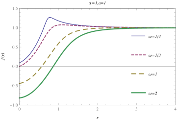
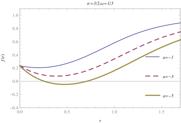
(a)		(b)
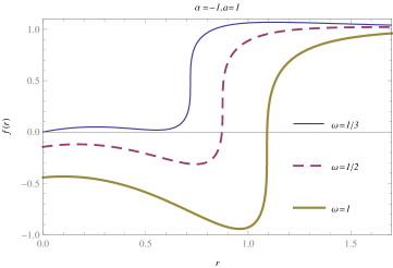
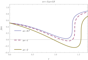
(c)		(d)

Figure 1: Plots show a metric function $f(r)$ as a function of $r$ for different values of parameters.

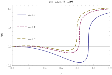
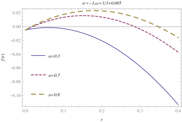
(a)		(b)

Figure 2: Plots show that for $a>0$, $\alpha<0$ and $\omega-\alpha^{2}/3>0$ there can exist maximum three horizons in the region $r<r_{*}$.

In the case that a singularity is covered by a horizon, the condition $\omega-2ar_{0}/5-r_{0}^{4}/3\geq 0$ must be satisfied and it gives the lower bound of mass, unless $\frac{2}{5}ar_{0}+\frac{1}{3}r^{4}_{0}<0$,

$$\omega_{m}\equiv\frac{2}{5}ar_{0}+\frac{1}{3}r^{4}_{0}.$$ (30)

If $\omega_{m}<0$ the lower bound for $\omega$ must be taken to be zero.

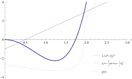
Figure 3: The plot illustrates that horizons can be obtained from intercepts between $l_{1}=r^{4}-r^{2}_{0}r^{2}$ and $l_{2}=-\frac{2}{5}ar+\omega-\frac{1}{3}r^{4}_{0}$

Fig. 1 shows behaviours of the metric function $f(r)$ with different values of parameters.

V Thermodynamics of black holes

In this section we present thermodynamic properties of the Lovelock black hole solution Eq. (27). As we demonstrate in the following, like any other black holes it also has thermodynamic properties. The Arnowitt-Deser-Misner(ADM) mass is defined

$$M=\frac{(D-2)V_{D-2}}{16\pi}\omega,$$ (31)

where $V_{D-2}=2\pi^{(D-1)/2}\Gamma[(D-1)/2]$ is the area of a unit $(D-2)$-sphere. Thus the gravitational mass of the black hole is determined by $f(r_{h})=0$, which in terms of a horizon $r_{h}$, from Eq. (27), reads

$$M=\frac{1}{16}\pi^{2}\left(2ar_{h}+\frac{5}{3}\alpha^{2}+5r_{h}^{4}+5\alpha r_{h}^{2}\right).$$ (32)

As $a\to 0$, Eq. (32) becomes

$$M\to\frac{5}{16}\pi^{2}\left(\frac{1}{3}\alpha^{2}+r_{h}^{4}+\alpha r_{h}^{2}\right),$$

which is found in Li:2011uk in the limits of the vanishing Born-Infield electromagnetic field and cosmological constant, $(\beta,\Lambda)\to 0$. Furthermore, in the limits $(a,\alpha)\to 0$ it leads to $M\to\frac{5}{16}\pi^{2}r^{4}_{h}$, which is mass for the Schwarzschild black hole in seven dimension Myers:1988ze . Imposing positive mass condition gives either possible range of horizon radii or mass, for fixed $a$ and $\alpha$. If the mass function $M(r_{h})$ has zeros, it will be critical points telling us which range of horizons is allowed. If the minimum of the mass function is positive it gives the minimum mass. Let us first think about the case $\alpha>0$, where a singularity is not covered by a horizon. For $\alpha>0$ and $a\geq 0$ the minimum mass is $\frac{5}{16}\pi^{2}\frac{1}{3}\alpha^{2}$. For $\alpha>0$ and $a<0$ the mass function can have two zeros, which means that it has zero minimum mass and there is no horizon between such two zeros. Next consider $\alpha<0$. If one is concerned with case that a singularity is covered by a horizon, in this case the minimum mass is $M(r_{0})$, which can be found in Eq. (30).

$$M_{m}=\frac{1}{16}\pi^{2}\left[2a(-\alpha)^{1/2}+\frac{5}{3}\alpha^{2}\right].$$ (33)

In Fig. 4 mass function $M(r_{h})$ is plotted as a function of $r_{h}$ for different values of $(a,\alpha)$.

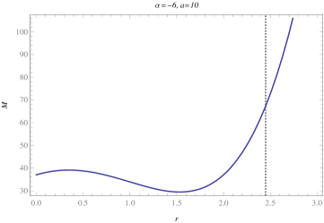
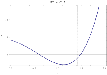
(a)		(b)
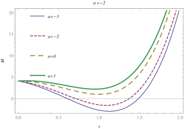
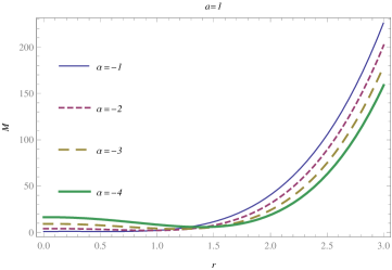
(c)		(d)

Figure 4: Plots show mass $M$ as a function of a horizon radius for different values of parameters. The dotted vertical lines in (a) and (b) correspond to $r=r_{0}$.

The Hawking temperature associated with a black hole is calculated using $T_{h}=\kappa/2\pi$, where $\kappa$ is a surface gravity of a horizon. Hence, the temperature $T_{h}$ at the horizon can be calculated by the definition $T_{h}=f^{\prime}(r_{h})/4\pi$, which is simplified to

$$T_{h}=\frac{a+10r^{3}_{h}+5\alpha r_{h}}{10\pi(\alpha+r^{2}_{h})^{2}}.$$ (34)

From Eq. (32) the positivity of mass means $ar_{h}>-\frac{5}{6}\alpha^{2}-\frac{5}{2}r_{h}^{4}-\frac{5}{2}\alpha r_{h}^{2}$. This leads to the inequality, $r_{h}(a+10r^{3}_{h}+5\alpha r_{h})>5\left(\frac{3}{2}r_{h}^{4}+\frac{1}{2}\alpha r_{h}^{2}-\frac{1}{6}\alpha^{2}\right)$. One can easily see that the right hand side in the inequality is positive for $r_{h}>r_{0}$, i.e., $a+10r^{3}_{h}+5\alpha r_{h}>0$. Thus, $T>0$ for $r_{h}>r_{0}$. Therefore, for $r_{h}>r_{0}$ whenever mass is positive, temperature is also positive. In the limit $a\to 0$, the temperature, Eq. (34) goes to

$$T_{h}\to\frac{2r^{3}_{h}+\alpha r_{h}}{2\pi(\alpha+r^{2}_{h})^{2}},$$

which is found in Li:2011uk as $(\beta,\Lambda)\to 0$. In addition the limit $\alpha\to 0$ further reduces it to the temperature for the Schwarzschild black hole, $T_{h}\to 1/\pi r_{h}$. Fig. 5 plots show the Hawking temperature of the black holes for different values of parameters.

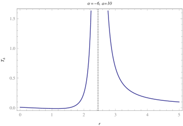
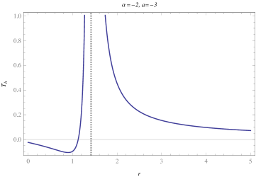
(a)		(b)
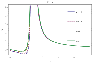
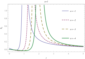
(c)		(d)

Figure 5: Plots show the Hawking temperature of the black holes, $T_{h}$ as a function of a horizon radius for different values of parameters. The dotted vertical lines in (a) and (b) correspond to $r=r_{0}$.

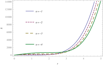
Figure 6: The plot shows entropy as a function of a horizon radius with different values of $\alpha$.

For the Schwarzschild black hole in $D$ dimension, the entropy of a black hole, $S$ is given by $S=A_{h}/4$ with the area of the horizon, $A_{h}$, which is $D-2$ dimensional surface area of a sphere. However, the black hole is supposed to obey the first law of thermodynamics $dM=TdS$. To calculate the entropy, the integral can be done with respect to $r_{h}$,

$$S=\int\frac{dM}{T}=\int T^{-1}\frac{\partial M}{\partial r_{h}}{dr_{h}}.$$ (35)

$\frac{\partial M}{\partial r_{h}}=\frac{1}{16}\pi^{2}(2a+20r^{3}_{h}+10\alpha r_{h})$ leads to

$$S=\int^{r_{h}}_{0}dr\frac{5}{4}\pi^{3}\left(\alpha+r^{2}\right)^{2}+\text{const.}=\frac{1}{12}\pi^{3}\left[3r_{h}^{5}+10\alpha r_{h}^{3}+15\alpha^{2}r_{h}\right]+\text{const.}.$$ (36)

Here we calculate the entropy by integration from $0$ to $r_{h}$. This is a usual way to define entropy in order to make entropy vanish when a horizon length becomes zero. Although a horizon length must be greater than $r_{0}$ it should not be a concern here because the difference is only an additive constant. The integrand in $S$ is positive, so $S\geq 0$ in any case. Also, it is worthwhile to notice that the entropy is independently expressed of $a$. A similar case happens in Li:2011uk . Actually it can be seen that this property holds in the general Lovelock theory for any static, spherically symmetric energy momentum tensor, THLee:2015 . The entropy expression in Li:2011uk coincides with Eq. (36). Using the areas of spheres $A_{n}=2\pi^{(n+1)/2}r^{n}/\Gamma[(n+1)/2]$ for an $n$ dimensional surface $A_{5}=\pi^{3}r^{5}$. Only the second term $\frac{1}{4}\pi^{3}r_{h}^{5}$ in Eq. (36) reflects the area law $S=A_{h}/4$ and the rest are usually considered as quantum corrections in higher dimension. Fig. 6 plots behaviours of the entropy in terms of a horizon radius for different values of $\alpha$.

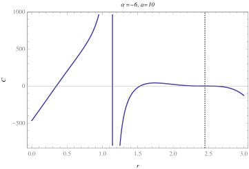
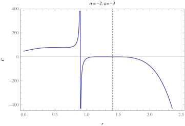
(a)		(b)
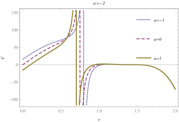
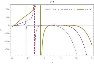
(c)		(d)

Figure 7: Plots show heat capacity as a function of a horizon radius with different values of parameters. The dotted vertical lines in (a) and (b) correspond to $r=r_{0}$.

The heat capacity is expressed by,

$$C=\frac{\partial M}{\partial T}=\frac{\partial M}{\partial r_{h}}\Big{/}\frac{\partial T}{\partial T_{h}}.$$ (37)

Using $\frac{\partial M}{\partial r_{h}}$ and $\frac{\partial T_{h}}{\partial r_{h}}=\frac{5\alpha^{2}-4ar_{h}-10r^{4}_{h}+15\alpha r^{2}_{h}}{10\pi\left(\alpha+r^{2}_{h}\right)^{3}}$, we get

$$C=-\frac{5\pi^{3}\left(\alpha+r^{2}_{h}\right)^{3}\left[a+5\left(2r^{3}_{h}+\alpha r_{h}\right)\right]}{4\left[4ar_{h}+5\left(-\alpha^{2}+2r^{4}_{h}-3\alpha r^{2}_{h}\right)\right]}.$$ (38)

In the limit $a\to 0$, the heat capacity Eq. (38) goes to

$$C\to-\frac{5}{4}\pi^{3}\frac{(\alpha+r^{2}_{h})^{3}(2r^{3}_{h}+\alpha r)}{(-\alpha^{2}+2r^{4}_{h}-3\alpha r^{2})},$$

which is found in Li:2011uk as $(\beta,\Lambda)\to 0$. We have just seen above that from the positive mass condition, $a+5(2r^{3}_{h}+\alpha r_{h})>0$ for $r_{h}>r_{0}$. Using the same condition, we notice that in the denominator in Eq. (38), for $r_{h}>r_{0}$

$$4ar_{h}+5(-\alpha^{2}+2r^{4}_{h}-3\alpha r^{2}_{h})>-\frac{25}{3}\alpha\left(r^{2}_{h}+\frac{\alpha}{3}\right).$$

The right hand side is always positive when $\alpha<0$ and $r_{h}>r_{0}$, which makes $C<0$, while when $\alpha>0$, $C$ can be either positive or negative. Therefore, the heat capacity is always negative for $r_{h}>r_{0}$ and $\alpha<0$ with positive mass and hence the black hole is thermodynamically unstable in positive mass region. However, it does not necessarily mean that the black hole is unstable as the Schwarzschild black hole is stable. The heat capacity of the black holes is plotted in Fig. 7 for various values of the parameters $(a,\alpha)$. It turns out that the parameters $(a,\alpha)$ influence the thermodynamic stability of black holes. There exist transition points at which a sign of heat capacity changes, i.e. boundaries between thermodynamically stable and unstable regions.

Let us define a transition point $r_{t}$ and a critical point $r_{c}$ such that $C$ becomes zero and diverges, respectively. $r_{c}$ is within the positive mass region but $r_{t}$ does not always belong to it. $r_{t}$ can occurs at either $A(r_{t})=(\alpha+r^{2}_{t})^{3}=0$ or $B(r_{t})=a+5\left(2r^{3}_{t}+\alpha r_{t}\right)=0$, which makes temperature zero. We saw that the positive mass condition guarantees $B$ is positive for $r_{h}>r_{0}$. There always exists one and only one $r_{c}$ for any $a$ at $D(r_{c})=4ar_{c}+5\left(-\alpha^{2}+2r^{4}_{c}-3\alpha r^{2}_{c}\right)=0$.

For $\alpha>0$, we can see that $A>0$ and $r_{c}>r_{t}$ if $r_{t}$ exists. Signs of $C$ are changing like $(-,0(r_{t}),+,0(r_{c}),-)$, from $-\infty$ to $\infty$.

For $\alpha<0$ when the positive mass condition imposed there is no zero in $B$ for $r_{t}>r_{0}$, which is the non-naked singularity condition, so $r_{0}$ is the only zero point satisfying both the positive mass and non-naked singularity conditions. Fig. 8 shows how heat capacity behaviour changes with $a$ after some critical values $a_{c}$. For $|a|>a_{c}$, $r_{c}>r_{t}$ while for $|a|<a_{c}$, $r_{c}<r_{t}$. For $|a|<a_{c}$ and $r_{c}\simeq r_{0}$ $C$ changes much less as $a$ changes for $r_{h}>r_{0}$.

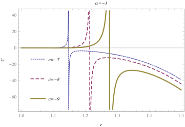
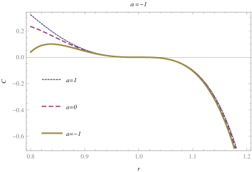
(a)		(b)

Figure 8: Plots show how heat capacity changes in different ranges of $a$.

VI Conclusion

The Lovelock theory is a natural extension of the Einstein theory of general relativity to higher dimensions and it is of a great arena for theoretical physics research. The Lovelock theory describes string-inspired corrections of the Einstein-Hilbert action and hence admits the general relativity as a particular case. In this paper, we have obtained exact static, spherically symmetric black hole solutions to the third order Lovelock gravity in a string cloud background in seven dimensions with help of carefully choosing coefficients of the curvature correction terms, thereby generalizing the static, spherically symmetric black hole solutions for these theories. These solutions possess rich properties of black holes and in the limits go over to black holes in Einstein’s gravity.

The string cloud parameter $a$ changes the number of horizons and singularities. For $\alpha>0$, $a$ can change the maximum number of horizons and the positivity of $a$ creates a singularity. In this case a singularity, if any, is naked. For $\alpha<0$ there is an interesting property. A horizon cannot exists between $r_{0}=|\alpha|^{1/2}$ and a singular point $r_{*}$ and hence we need know only whether a horizon is ahead or behind from $r_{0}$ instead of $r_{*}$ in order to see whether a singularity is naked. There is only one singularity. For $a\geq 0$ when a singularity is non-naked there should be only one horizon. For $a<0$, when a singularity is non-naked, the singularity must be between two horizons.

We proceeded to find exact expressions for the thermodynamic quantities like the black hole mass, the Hawking temperature, entropy and heat capacity and in turn also analysed the thermodynamic stability of black holes. In addition we explicitly brought out the effect of a string cloud background on black hole solutions and their thermodynamics.

We found that a positive mass condition leads to positive temperature for $r_{h}>r_{0}$, which is a condition for a non-naked singularity for $\alpha<0$. The entropy does not depend on a string cloud. This result can be extended for any spherical and static source in the Lovelock theory THLee:2015 . We also see the entropy does not obey the horizon area formula. For heat capacity, $\alpha>0$ a critical(singular) point $r_{c}$ is greater than a transition (zero) point $r_{t}$ and for $\alpha<0$ when a positive mass and a non-naked singularity conditions applied, $r_{t}=r_{0}$ and there is no $r_{c}$. In this case the heat capacity is negative, telling us that the black hole is thermodynamically unstable like the Schwarzschild black hole.

The possibility of a further generalization of these results in arbitrary dimensional Lovelock gravity is an interesting problem for future research.

- (1) S. W. Hawking, Nature 248, 30 (1974).
- (2) S. Hawking, D. N. Page, Commun. Math. Phys. 87, 577 (1983)
- (3) D. Lovelock, J. Math. Phys. 12, 498 (1971).
- (4) H. A. Buchdahl, Mon. Not. Roy. Astron. Soc. 150, 1 (1970).
- (5) D. J. Gross and E. Witten, Nucl. Phys. B 277, 1 (1986).
- (6) R. Emparan and H. S. Reall, Living Rev. Rel. 11, 6 (2008).
- (7) B. Zwiebach, Phys. Lett. B 156, 315 (1985).
- (8) D.G. Boulware, S. Deser, Phys. Rev. Lett. 55, (1985) 2656; J.T. Wheeler, Nucl. Phys. B 268, (1986) 737; R.C. Myers, J.Z. Simon, Phys. Rev. D 38, (1988) 2434.
- (9) J. T. Wheeler, Nucl. Phys. B 273, 732 (1986).
- (10) J. T. Wheeler, Nucl. Phys. B 268, 737 (1986).
- (11) R. C. Myers and J. Z. Simon, Phys. Rev. D 38, 2434 (1988).
- (12) S. H. Mazharimousavi, O. Gurtug and M. Halilsoy, Int. J. Mod. Phys. D 18, 2061 (2009).
- (13) M. H. Dehghani, N. Alinejadi and S. H. Hendi, Phys. Rev. D 77, (2008) 104025; S. H. Hendi and M. H. Dehghani, Phys. Lett. B 666, (2008), 116; M. M. Anber and D. Kastor, JHEP 05, 061 (2008); R. G. Cai, L. M. Cao, Y. P. Hu and S. P. Kim, Phys. Rev. D 78, (2008), 124012; S. H. Mazharimousavi and M. Halilsoy, Phys. Lett. B 665 (2008), 125; C. Garraffo, G. Giribet, E. Gravanis and S. Willison, J. Math. Phys. 49 (2008), 042502; G. Kofinas and R. Olea, JHEP 11, (2007), 069; Q. Exirifard and M. M. Sheikh-Jabbari, Phys. Lett. B 661 (2008), 158.
- (14) R. G. Cai, Phys. Lett. B 582, 237 (2004).
- (15) R. G. Cai, Phys. Rev. D 65, 084014 (2002) [hep-th/0109133].
- (16) R. G. Cai and Q. Guo, Phys. Rev. D 69, 104025 (2004) [hep-th/0311020].
- (17) P. Li, R. H. Yue and D. C. Zou, Commun. Theor. Phys. 56, 845 (2011).
- (18) X. O. Camanho and J. D. Edelstein, Class. Quant. Grav. 30, 035009 (2013) [arXiv:1103.3669 [hep-th]].
- (19) X. O. Camanho, J. D. Edelstein, J. Maldacena and A. Zhiboedov, arXiv:1407.5597 [hep-th].
- (20) R. G. Cai and K. S. Soh, Phys. Rev. D 59, 044013 (1999)
- (21) P. S. Letelier, Phys. Rev. D 20, 1294 (1979).
- (22) E. Herscovich and M. G. Richarte, Phys. Lett. B 689, 192 (2010).
- (23) S G. Ghosh and S. D. Maharaj, Phys. Rev. D 89, 084027 (2014).
- (24) S. G. Ghosh, U. Papnoi and S. D. Maharaj, Phys. Rev. D 90, 044068 (2014).
- (25) B. Zwiebach, Phys. Lett. B 156 (1985) 315; B. Zumino, Phys. Rept. 137 (1986) 109; N. Deruelle and L. Farina-Busto, Phys. Rev. D 41 (1990) 3696; G. A. MenaMarugan, ibid. 46 (1992) 4320; 46 (1992) 4340; R. G. Cai and N. Ohta, Phys. Rev. D 74 (2006) 064001.
- (26) J. L., Synge, in Relativity: the General Theory, (North-Holland, Amsterdam, 1996), p.175.
- (27) M. Salgado, Class. Quant. Grav. 20, 4551 (2003) [gr-qc/0304010].
- (28) Tae-Hun Lee, Sushant G. Ghosh, Sunil Maharaj and Dharmanand Baboolal “Thermodynamics of the Lovelock black holes ” in preparation.