Contagion in an interacting economy

Abstract

We investigate the credit risk model defined in [1] under more general assumptions, in particular using a general degree distribution for sparse graphs. Expanding upon earlier results, we show that the model is exactly solvable in the $N\rightarrow\infty$ limit and demonstrate that the exact solution is described by the message-passing approach outlined in Karrer and Newman [2], generalized to include heterogeneous agents and couplings. We provide comparisons with simulations of graph ensembles with power-law degree distributions.

1 Introduction

Modern economies form complex, heavily interconnected ecosystems perhaps best epitomized by the extraordinary intricacies of supply chains, routinely involving hundreds of suppliers in dozens of countries. But as highlighted by Haldane and May [3], complexity is associated with greater systemic instability, and the crisis of 2007-2009 made it clear that proper analysis of systemic risk is needed. Accordingly, financial contagion and credit-risk modeling is a long-standing research subject [4] that has recently attracted renewed interest [5, 6, 7, 8, 9].

Credit events cluster in times of economic stress, resulting in large aggregate losses that are not captured by the risk rating (e.g. S&P) of individual institutions. As a result, attempts at regulatory controls in the spirit of the Basel II capital requirements should take into account the possibility of mutually dependent defaults in order to adequately model the risk of large portfolios. Historical approaches in financial risk analysis include replacing the number of firms in a portfolio by a reduced effective number, or to condition the default probability on macro-economic indicators [10, 11]. Multi-factor Merton models correlate defaults by assuming that asset returns of different firms undergo correlated random walks [4, 12] and that default occurs when the asset level falls below the debt threshold. But while these models do take into account correlations, they are not causal and can thus fail to capture systemic fragility, i.e. the effect of the collapse of a single entity or group of entities on the entire network.

The physical perspective spurred by the development of econophysics is somewhat different, focusing more on system-wide risk through interactions between agents than on individual risks [13, 14]. In particular, there has been in the past twenty years an intensive research effort on the network structure of social and economic interactions, e.g. the structure of sexual contacts, of academic citations or of the internet [15, 16, 17, 18], showing that the number of neighbors or partners of an individual (or node) in most social networks follows a power-law distribution. This is sometimes explained as the result of a preferential attachment in the network formation process, as in the Barabási-Albert model [19].

In this context, a natural framework for systemic risk is provided by contagion processes on graphs defined by economic interactions: given such processes, one is interested in the fraction of the network likely to be affected over a certain time horizon. This approach has been used for example by Gai and Kapadia [5, 20], modeling the banking network as a directed weighted network of exposures in which banks fail if they are overexposed to failed banks. The fraction of vulnerable banks can then be determined through a generating function method of the type used by Moore and Newman [21, 22] to study SIR models on graphs. Caccioli et al. [8] use a representation of the banking system as a bipartite network of assets and banks where distressed banks sell assets, which lower the price of assets and thus deteriorates the balance sheet of other banks and precipitates them into distress in turn. Hatchett and Kühn [1] investigate contagion in networks of firms via pairwise general economic interactions that include, but are not restricted to, financial exposures, where default of neighbors strongly enhance a node’s intrinsic probability of default. Contagion on networks, while a relatively heterogeneous set of phenomena, has nevertheless been largely successfully analyzed using tools from statistical mechanics and computer science such as message-passing [23, 24]. In the context of infection dynamics for example, Altarelli et al.[25] evaluate the efficiency of targeted immunization strategies; Karrer and Newman [2] derive analytic solution for the susceptibility of a network to SIR-type epidemics.

We focus in this paper on the model developed in Hatchett and Kühn [1], which investigates how networks of economic interactions affect the system-wide default likelihood across economic cycles. That investigation provided an analytic description of the average fraction of defaulted firms in the limit of “dilute yet large” connectivity, i.e. for networks where the average number $c$ of neighbors is large ($c\rightarrow\infty$), but small compared to the size of the system ($\tfrac{c}{N}\rightarrow 0$). Moreover, the analysis was limited to Erdös-Rényi random graphs rather than more realistic heavy-tailed degree distributions such as were found by Caccioli et al. for the Austrian banking network [26], or by Souma et al. for links between parent companies and subsidiaries, or between banks and firms in Japan [27]. In what follows we will study networks with heavy tailed degree distributions and finite mean degrees.

The model has several attractive features: contagion dynamics is not exclusively driven by an initial shock; it reveals that systemic risk, while clearly dependent on the system-wide distribution of exposures and connectivities, will be relatively insensitive to individual dependencies; the model provides a clear mechanism for default clustering; and (as we shall show in what follows) it is analytically tractable for a larger class of specifications than originally considered in [1]. Moreover, other models such as the Centola-Macy [28] or Watts [29] models, in which contagion is triggered whenever the number (resp. the fraction) of contaminated neighbors exceeds a certain threshold, can be recovered by taking adequate limits, making it a valuable toy model. Many of its parameters can also be inferred in principle by suitable rating procedures. Unlike other approaches however it does not look into the ’micro-structure’ of contagion as generated e.g. by overlapping portfolios which are the main focus of Caccioli et al.[8], or by similarities in trading strategies. We believe, however, that it can be straightforwardly generalized to include such effects at least on a qualitative level and propose a possible approach in the following.

The remainder of the paper is organized as follows: in section 2, we define our model and set up the formalism to analyze its dynamics. In section 3, we provide an analytic solution for general degree distributions (with finite or infinite connectivity) using recently developed methods in dynamic message-passing, known to be exact when the underlying network is a tree and generally accurate on a large number of graph ensembles. In section 4, we provide numerical results, and summarize our findings in section 5. In the appendix we use a generating functional analysis to demonstrate that the message-passing solution is the correct infinite-network limit for a configuration model random graph.

2 Model definitions

Our model consists of an ensemble of locally tree-like weighted random graphs $G=(V,E)$ with edge weights $\left(w_{ij},w_{ji}\right)$ drawn according to some distribution $p_{w}\left(w_{ij},w_{ji}\right)$. In the context of modeling credit contagion, the nodes describe the entities acting in the economy, whether they be banks, hedge funds or firms. An edge $(ij)$ can be thought of as a partnership or joint investment where firm $i$ has a stake $w_{ij}$ and firm $j$ has a stake $w_{ji}$ (which needs not be equal to $w_{ij}$). If one of the partners defaults, the other partner writes its stake as a financial loss. For example, one may think of a pair of nodes as a supplier of raw goods and a manufacturer: if the supplier defaults, the need for the manufacturer to find other suppliers to its specifications has a direct financial effect, while obviously losing a client would be a blow to the supplier’s balance sheet.

To each node we associate a threshold $\theta_{i}$ and a binary variable $n_{i,t}\in\left\{0,1\right\}$ signifying whether the node is active ($n_{i,t}=0$) or defaulted ($n_{i,t}=1$), the threshold $\theta_{i}$ corresponding to the assets of node $i$ at the start of the risk horizon. We write $\mathbf{A}=\left\{a_{ij}\right\}$ for the adjacency matrix of the graph. The degree distribution of the graph will be kept general in the derivation of analytical results. For numerical results however, a power-law distribution with exponent $\gamma=3$ and hard cutoffs is used in order to model the fat-tailed distributions seen in such settings (see e.g. [30]).

In a Merton model, firms are considered as holding debt that must be repaid after a fixed time period. If their wealth at this time is below the value of the debt, they default, wealth being modeled as an initial wealth plus a Gaussian random variable. As in a Merton model, we assume that firms default when their wealth, i.e. their initial wealth minus the losses incurred due to the default of their neighbors, plus a random noise term, falls to zero or below. We write the wealth at time $t$ as

$$\theta_{i,t}=\theta_{i}+\eta_{i,t}-\sum_{\begin{subarray}{c}j\end{subarray}}a_{ij}w_{ij}n_{j,t}\ .$$ (1)

Because of the presence of the noise, defaults are random events. The noise variable $\eta_{i,t}$ has the form

$$\eta_{i,t}=\xi_{0,t}+\xi_{i,t}\ .$$ (2)

The $\xi_{0,t}$ are random variables that induce a correlation of the noise across the entire economy and thus represent the effect of varying global economic conditions. Unlike in the usual Merton model (which uses random walks to determine default probabilities within a one period model), we use a multi-period approach in which the $\left\{\xi_{i,t}\right\}$ are idiosyncratic noise variables for individual time steps. We take the $\left\{\xi_{i,t}\right\}$ to be i.i.d., although we can allow their distribution to vary with time. This decomposition of the noise corresponds to the minimal recommendations of the Basel II Accords [31].

The $n_{i,t}$ then evolve according to the dynamical rule

$$n_{i,t+1}=n_{i,t}+(1-n_{i,t})\Theta\left(-\theta_{i,t}\right)\ .$$ (3)

Written in this way the dynamics have $n_{i}=1$ as an absorbing state: if $n_{i,t_{0}}=1$ then for all $t>t_{0}$ we have $n_{i,t}=1$. From the modeling point of view, this irreversibility of default is a reasonable assumption for the limited time horizon considered here. This is a crucial point: thanks to this absorbing state, we have no memory effects and can obtain $\rho$ easily. Put another way, we go from having to consider an exponential $(2^{T})$ number of possible trajectories for each node to $T+1$ possible trajectories, resulting in an enormous simplification.

Our aim in this paper is to compute the fraction of defaulted nodes at a finite time horizon $T$, i.e to compute

$$\rho(T)=\dfrac{1}{N}\sum_{\begin{subarray}{c}i\end{subarray}}n_{i,T}\ ,$$ (4)

where $N=\left|V\right|$ is the number of firms in the economy. We will call $\rho(T)$ the defaulted fraction.

Given the way the model is set up, the trajectories $\left\{n_{i,t}\right\}$ undergo Markovian dynamics. Their joint probability factorizes as

$$P\left(\left\{n_{i,t}\right\}_{t=0,\cdots,T;\;i\in V}\right)=P(\left\{n_{i,0}\right\})\prod_{\begin{subarray}{c}t=1\end{subarray}}^{T}P\left(\left\{n_{i,t}\right\}_{i\in V}|\left\{n_{i,t-1}\right\}_{i\in V}\right)\ .$$

In what follows, we will omit giving ranges for the $i$ and $t$ subscripts.

As the $\xi_{i,t}$ are independent, we can integrate over them. The resulting transition probabilities at time $t$, $P\left(\left\{n_{i,t}\right\}|\left\{n_{i,t-1}\right\}\right)$, factorize over the sites as

$$P\left(\left\{n_{i,t}\right\}|\left\{n_{i,t-1}\right\}\right)=\prod_{\begin{subarray}{c}i\end{subarray}}p(n_{i,t}|n_{i,t-1},\left\{n_{j,t-1}\right\}_{j\in\partial i})\ ,$$

in which $\partial i$ denotes the set of neighbors of node $i$. As long as a node $i$ is active at time $t-1$, its transition probability $p(n_{i,t}|n_{i,t-1}=0,\left\{n_{j,t-1}\right\}_{j\in\partial i})$ depends on its local field

$$h_{i,t-1}=\sum_{\begin{subarray}{c}j\end{subarray}}a_{ij}w_{ij}n_{j,t-1}=\sum_{\begin{subarray}{c}j\in\partial i\end{subarray}}w_{ij}n_{j,t-1}\ ,$$

and on the threshold $\theta_{i}$, i.e. it will be of the form

$$p(n_{i,t}=1|n_{i,t-1}=0,\left\{n_{j,t-1}\right\}_{j\in\partial i})=W_{t-1}\left(h_{i,t-1}-\theta_{i}\right)\ ,$$

where $W_{t-1}$ is a function whose exact form depends on the distribution of the noise $\eta_{i,t-1}$ at time $t-1$.

Conversely, for nodes that are defaulted at time $t-1$, the single-site transition probabilities are independent of their local fields and are simply given by

$$p(n_{i,t}|n_{i,t-1}=1,\left\{n_{j,t-1}\right\}_{j\in\partial i})=\delta_{n_{i,t},1}\ ,$$

reflecting the irreversible nature of the dynamics in the sense described above (with $n_{i,t}=1$ as absorbing state).

Writing $\mathbf{n}_{i}=(n_{i,0},n_{i,1},\cdots,n_{i,T})$, we find it advantageous to parametrize the paths $\mathbf{n}_{i}$ by a single default time $t_{i}$ defined as the time for which $n_{i,t<t_{i}}=0$ and $n_{i,t_{i}}=1$. Moreover we will assume $\left\{n_{i,0}\right\}_{i\in V}=0$ in the remainder of this article, and omit the dependence on initial conditions (which simply forbid the default time $t_{i}=0$). Under these assumptions, we can write the path probabilities as default-time probabilities:

$$P\left(\left\{n_{i,t}\right\}\right)=P(\left\{n_{i,0}\right\})P(\left\{t_{i}\right\}|\left\{n_{i,0}\right\})=\prod_{\begin{subarray}{c}i\end{subarray}}P(t_{i}|\theta_{i},\mathbf{h}_{i})\ ,$$

where

$$P(t_{i}|\theta_{i},\mathbf{h}_{i})=W_{t_{i}-1}\left(h_{i,t_{i}-1}-\theta_{i}\right)\prod_{\begin{subarray}{c}s=0\end{subarray}}^{t_{i}-2}\left[1-W_{s}\left(h_{i,s}-\theta_{i}\right)\right]\ ,$$ (5)

and where we have introduced the notation $\mathbf{h}_{i}=\left\{h_{i,s}\right\}_{s=0,\cdots,T-1}$.

Additionally, we must include the special case where a node does not default within the time horizon T, corresponding to the path $n_{i,t}=0$ for all $t\leq T$. The probability of such a “survival” path of node $i$ is given by

$$P({\rm Survival}|\theta_{i},\mathbf{h}_{i})=\prod_{\begin{subarray}{c}s=0\end{subarray}}^{T-1}\left[1-W_{s}\left(h_{i,s}-\theta_{i}\right)\right]\ .$$ (6)

In any sum over default times, the survival path will be implicitly included (it can be straightforwardly mapped onto a default time $t=T+1$ by setting $W_{T}=1$).

The functions $W_{t}$ encode the noise of the model: in the case where the noise $\xi_{i,t}$ is Gaussian, which will be our reference, we have

$$W_{t}(x)=\Phi\left(x-\xi_{0,t}\right)$$ (7)

where $\Phi$ is the Gaussian cumulative distribution function (cdf), whereas a deterministic model would have $W_{t}(x)=\Theta(x)$ where $\Theta$ is the Heaviside function.

We can remark at this point that the $W_{t}$ need not in general be defined in terms of a cdf and can be arbitrary transition probabilities, e.g. they need not be monotone with respect to the local field. Indeed, whatever the choice of the $W_{t}$ we remain within the scope of 2-states unidirectional models as defined in [32].

Moreover, bootstrap percolation is recovered by having $P(\mathbf{n_{0}})$ (or equivalently $W_{0}$) be a suitable seeding probability, taking constant couplings $w_{ij}=w_{0}$ and wealth $\theta_{i}=\theta_{0}$, taking the zero-noise limit and setting $\theta_{0}w_{0}^{-1}=c$ for a constant $c$ corresponding to the number of defaulted (infected) neighbors needed to propagate default. For a Watts-type percolation, $\theta=k\theta_{0}$ should be considered instead with $k$ being the node’s degree.

In the usual SI model, a node $i$ has a probability per time step $\mu_{ij}$ to be infected by an infected neighbor, and this can be represented within the current framework by choosing $w_{ij}=-\log(1-\mu_{ij})$, $\theta=0$ and $W_{t}(x)=1-\exp\left(-x\right)$, along with a suitable change in distribution of the $w_{ij}$ to reflect the desired distribution of the $\mu_{ij}$.

3 Message-passing approach

The following approach is an extension of a method proposed by Karrer and Newman [2], adapted to apply to systems with bond disorder. Simpler versions of the resulting equations for homogeneous systems (no bond disorder and uniform degree) appear in Ohta and Sasa [33]. In Altarelli et al. [34] and Lokhov et al. [32], the equations are derived for the single-instance case (without graph ensemble averaging) in the presence of bond disorder.

The result that includes graph ensemble averaging, and thus provides a description valid in the thermodynamic limit, can also be derived from generating functional analysis. In that derivation, the message-passing equations derived below appear as self-consistency equations in a saddle-point evaluation of a path-integral. Their detailed structure is a natural consequence of the dilute nature (relative to system size) of the connection pattern. This alternative derivation is provided in the appendix.

We consider a node $i$ of degree $k_{i}$ and the set of neighboring nodes $\left\{j\in\partial i\right\}$. In order to compute node $i$’s default probability at time $t$, we need the marginal default probability of each of the neighboring nodes $j$ at all times $\tau<t$, knowing that node $i$ only defaults at time $t$. But given the form of the dynamics, the marginal probabilities of defaulting at a time $t^{\prime}<t$ do not depend on the specific time of the default $t$, but only on the fact that it is posterior to the default time $t^{\prime}$. Thanks to this, it is very easy to compute marginals by forward-integration.

Consider a specific instance of a weighted tree $G$, and a node $i$ on this graph. We write $p_{i}(t_{i})$ for the probability for $i$ to default at $t_{i}$. If we now consider the neighbors of $i$, we can write that

$$p_{i}(t_{i})=\sum_{\begin{subarray}{c}\left\{\tau_{j}\right\}_{j\in\partial i}\end{subarray}}p_{i}(t_{i}|\left\{\tau_{j}\right\}_{j\in\partial i})\prod_{\begin{subarray}{c}j\in\partial i\end{subarray}}m^{j\rightarrow i}(\tau_{j}|t_{i})\ ,$$

where $m^{j\rightarrow i}(\tau_{j}|t_{i})$ is the probability that $j$ defaults at $\tau_{j}$ conditional on $i$ defaulting at $t_{i}$. The factorization of the neighbors’ conditional probabilities is due to the underlying graph being a tree. In terms of the specifications of the previous section, the conditional probability $p_{i}(t_{i}|\left\{\tau_{j}\right\}_{j\in\partial i})$ is simply $P\left(t_{i}|\theta_{i},\mathbf{h}_{i}\right)$ defined in (5).

Likewise, we can write

$$m^{j\rightarrow i}(\tau_{j}|t_{i})=\sum_{\begin{subarray}{c}\left\{\tau_{l}\right\}_{l\in\partial j\backslash i}\end{subarray}}p_{j}(\tau_{j}|t_{i},\left\{\tau_{l}\right\}_{l\in\partial j\backslash i})\prod_{\begin{subarray}{c}l\in\partial j\backslash i\end{subarray}}m^{l\rightarrow j}(\tau_{l}|\tau_{j})\ .$$ (8)

But we note that once a node has defaulted, the subsequent dynamics of its neighbors no longer influence it. In particular, the conditional probability $m^{l\rightarrow j}(\tau_{l}|\tau_{j})$ depends on $\tau_{j}$ only insofar as $\tau_{j}<\tau_{l}$. Hence,

$$\forall\tau_{j}>\tau_{l},\qquad m^{l\rightarrow j}(\tau_{l}|\tau_{j})=m^{l\rightarrow j}(\tau_{l}|\tau_{l})\equiv m^{l\rightarrow j}(\tau_{l})\ .$$ (9)

Likewise, we note that the conditional probabilities $p_{i}(t_{i}|\left\{\tau_{j}\right\}_{j\in\partial i})$ and $p_{j}(\tau_{j}|t_{i},\left\{\tau_{l}\right\}_{l\in\partial j\backslash i})$ only depend on the neighbors’ default times insofar as these precede their own, i.e.

$$p_{i}(t_{i}|\left\{\tau_{j}\right\}_{j\in\partial i})=p_{i}(t_{i}|\left\{\tau_{j};\,\tau_{j}<t_{i}\right\}_{j\in\partial i})\ ,$$

and it is clear that for all $l,j$,

$$\sum_{\begin{subarray}{c}\tau_{l}\geq\tau_{j}\end{subarray}}m^{l\rightarrow j}(\tau_{l}|\tau_{j})=1-\sum_{\begin{subarray}{c}\tau_{l}<\tau_{j}\end{subarray}}m^{l\rightarrow j}(\tau_{l}|\tau_{j})=1-\sum_{\begin{subarray}{c}\tau_{l}<\tau_{j}\end{subarray}}m^{l\rightarrow j}(\tau_{l})\ .$$

Using these results we can take a new look at the equation for the conditional probability $m^{j\rightarrow i}(\tau_{j}|t_{i})$ and evaluate the r.h.s. of eq. (8), expressing it in terms of the $m^{l\rightarrow j}(\tau_{l})$ for $\tau_{l}<\tau_{j}$. For all $r$ in the neighborhood of $j$ ($i$ excepted), we have

$$\sum_{\begin{subarray}{c}\left\{\tau_{l}\right\}_{l\in\partial j\backslash i}\end{subarray}} p_{j}(\tau_{j}|t_{i},\left\{\tau_{l}\right\}_{l\in\partial j\backslash i})\prod_{\begin{subarray}{c}l\in\partial j\backslash i\end{subarray}}m^{l\rightarrow j}(\tau_{l}|\tau_{j})$$

$$= \sum_{\begin{subarray}{c}\left\{\tau_{l}\right\}_{l\in\partial j\backslash\left\{i,r\right\}}\end{subarray}}\left[\sum_{\begin{subarray}{c}\tau_{r}<\tau_{j}\end{subarray}}p_{j}(\tau_{j}|t_{i},\left\{\tau_{l}\right\}_{l\in\partial j\backslash i})m^{r\rightarrow j}(\tau_{r}|\tau_{j})\prod_{\begin{subarray}{c}l\in\partial j\backslash\left\{i,r\right\}\end{subarray}}m^{l\rightarrow j}(\tau_{l}|\tau_{j})\right.$$

$$\left.\qquad+\sum_{\begin{subarray}{c}\tau_{r}\geq\tau_{j}\end{subarray}}p_{j}\left(\tau_{j}|t_{i},\left\{\tau_{l}\right\}_{l\in\partial j\backslash i}\right)m^{r\rightarrow j}(\tau_{r}|\tau_{j})\prod_{\begin{subarray}{c}l\in\partial j\backslash\left\{i,r\right\}\end{subarray}}m^{l\rightarrow j}(\tau_{l}|\tau_{j})\right]$$

$$= \sum_{\begin{subarray}{c}\left\{\tau_{l}\right\}_{l\in\partial j\backslash\left\{i,r\right\}}\end{subarray}}\left[\sum_{\begin{subarray}{c}\tau_{r}<\tau_{j}\end{subarray}}p_{j}\left(\tau_{j}|t_{i},\left\{\tau_{l}\right\}_{l\in\partial j\backslash i}\right)m^{{r\rightarrow j}}(\tau_{r})\prod_{\begin{subarray}{c}l\in\partial j\backslash\left\{i,r\right\}\end{subarray}}m^{l\rightarrow j}(\tau_{l}|\tau_{j})\right.$$

$$\left.\qquad+p_{j}\left(\tau_{j}|t_{i},\left\{\tau_{l}\right\}_{l\in\partial j\backslash\left\{i,r\right\}}\right)\left(\sum_{\begin{subarray}{c}\tau_{r}\geq\tau_{j}\end{subarray}}m^{r\rightarrow j}(\tau_{r}|\tau_{j})\right)\prod_{\begin{subarray}{c}l\in\partial j\backslash\left\{i,r\right\}\end{subarray}}m^{l\rightarrow j}(\tau_{l}|\tau_{j})\right]$$

$$= \sum_{\begin{subarray}{c}\left\{\tau_{l}\right\}_{l\in\partial j\backslash\left\{i,r\right\}}\end{subarray}}\left[\sum_{\begin{subarray}{c}\tau_{r}<\tau_{j}\end{subarray}}p_{j}(\tau_{j}|t_{i},\left\{\tau_{l}\right\}_{l\in\partial j\backslash i})m^{r\rightarrow j}(\tau_{r})\prod_{\begin{subarray}{c}l\in\partial j\backslash\left\{i,r\right\}\end{subarray}}m^{l\rightarrow j}(\tau_{l}|\tau_{j})\right.$$

$$\left.\qquad+p_{j}\left(\tau_{j}|t_{i},\left\{\tau_{l}\right\}_{l\in\partial j\backslash\left\{i,r\right\}}\right)\left(1-\sum_{\begin{subarray}{c}\tau_{r}<\tau_{j}\end{subarray}}m^{r\rightarrow j}(\tau_{r})\right)\prod_{\begin{subarray}{c}l\in\partial j\backslash\left\{i,r\right\}\end{subarray}}m^{l\rightarrow j}(\tau_{l}|\tau_{j})\right]\ .$$

Hence we can limit the sum over default times $\tau_{l}\leq T$ to a sum over default times $\tau_{l}\leq\tau_{j}$, and write

$$m^{j\rightarrow i}(\tau_{j}|t_{i})=\sum_{\begin{subarray}{c}\left\{\tau_{l}\right\}_{l\in\partial j\backslash i}\\ \tau_{l}\leq\tau_{j}\end{subarray}}p_{j}(\tau_{j}|t_{i},\left\{\tau_{l}\right\}_{l\in\partial j\backslash i})\prod_{\begin{subarray}{c}l\,|\tau_{l}<\tau_{j}\end{subarray}}m^{l\rightarrow j}(\tau_{l})\prod_{\begin{subarray}{c}l\,|\tau_{l}=\tau_{j}\end{subarray}}\left(1-\sum_{\begin{subarray}{c}\tau<\tau_{j}\end{subarray}}m^{l\rightarrow j}(\tau)\right)\ ,$$ (10)

whereas for $\tau_{j}<t_{i}$ we have

$$m^{j\rightarrow i}(\tau_{j})=\sum_{\begin{subarray}{c}\left\{\tau_{l}\right\}_{l\in\partial j\backslash i}\\ \tau_{l}\leq\tau_{j}\end{subarray}}p_{j}(\tau_{j}|\left\{\tau_{l}\right\}_{l\in\partial j\backslash i})\prod_{\begin{subarray}{c}l\,|\tau_{l}<\tau_{j}\end{subarray}}m^{l\rightarrow j}(\tau_{l})\prod_{\begin{subarray}{c}l\,|\tau_{l}=\tau_{j}\end{subarray}}\left(1-\sum_{\begin{subarray}{c}\tau<\tau_{j}\end{subarray}}m^{l\rightarrow j}(\tau)\right)\ .$$ (11)

Replacing $p_{j}(\tau_{j}|\left\{\tau_{l}\right\}_{l\in\partial j\backslash i})$ by its more explicit version $P\Big{(}\tau_{j}|\,\theta_{j},\sum_{\begin{subarray}{c}l\in\partial j\backslash i\end{subarray}}w_{l}\mathbf{n}_{l}\Big{)}$, this is expressed as

$$m^{j\rightarrow i}(\tau_{j})=\sum_{\begin{subarray}{c}\left\{\tau_{l}\right\}_{l\in\partial j\backslash i}\\ \tau_{l}\leq\tau_{j}\end{subarray}}P\Big{(}\tau_{j}\big{|}\,\theta_{j},\sum_{l\in\partial j\backslash i}w_{l}\mathbf{n}_{l}\Big{)}\prod_{\begin{subarray}{c}l\,|\tau_{l}<\tau_{j}\end{subarray}}m^{l\rightarrow j}(\tau_{l})\prod_{\begin{subarray}{c}l\,|\tau_{l}=\tau_{j}\end{subarray}}\left(1-\sum_{\begin{subarray}{c}\tau<\tau_{j}\end{subarray}}m^{l\rightarrow j}(\tau)\right)\ .$$ (12)

This single-instance equation can be solved by forward propagation from initial conditions for all nodes, as in [32] for a number of models. It has been remarked in several contexts that message-passing works rather well even if the graph is only locally tree-like.

Here, we average instead over the degree and wealth of the associated nodes, as well as the coupling strengths, to obtain the typical behavior of the system in the infinite system size limit $N\rightarrow\infty$.

We note that the neighbors’ degree distribution is different from that of a node chosen at random: the probability for a neighbor to have degree $k$ is $\tfrac{kp_{k}}{\left\langle k\right\rangle}$. Thus the average $m(\tau)$ of $m^{j\rightarrow i}(\tau)$ satisfies the recursion

$$m(\tau)\equiv \sum_{\begin{subarray}{c}k\end{subarray}}\frac{kp_{k}}{\left\langle k\right\rangle}\sum_{\begin{subarray}{c}\tau_{1},\cdots,\tau_{k-1}\leq\tau\end{subarray}}\;\prod_{\begin{subarray}{c}l|\tau_{l}<\tau\end{subarray}}m(\tau_{l})\prod_{\begin{subarray}{c}l|\tau_{l}=\tau\end{subarray}}\left(1-\sum_{\begin{subarray}{c}\tau^{\prime}<\tau\end{subarray}}m(\tau^{\prime})\right)\left\langle P\left(\tau\Big{|}\,\theta,\sum_{\begin{subarray}{c}l=1\end{subarray}}^{k-1}w_{l}\mathbf{n}(\tau_{l})\right)\right\rangle_{\theta,\left\{w_{l}\right\}}\ ,$$ (13)

where the average over the couplings $\left\langle\cdots\right\rangle_{\left\{w_{l}\right\}}$ is done over the marginal coupling distribution.

The resulting equation is forward-propagating in $m$, starting from $m(1)=\left\langle W_{0}(-\theta)\right\rangle_{\theta}$. The average fraction of defaults happening at time $t$, meanwhile, is given by

$$p(t)\equiv \dfrac{1}{N}\sum_{\begin{subarray}{c}i\end{subarray}}p_{i}(t)$$

$$= \sum_{\begin{subarray}{c}k\end{subarray}}p_{k}\sum_{\begin{subarray}{c}\tau_{1},\cdots,\tau_{k}\leq t\end{subarray}}\;\prod_{\begin{subarray}{c}l|\tau_{l}<t\end{subarray}}m(\tau_{l})\prod_{\begin{subarray}{c}l|\tau_{l}=t\end{subarray}}\left(1-\sum_{\begin{subarray}{c}\tau^{\prime}<t\end{subarray}}m(\tau^{\prime})\right)\left\langle P\left(t\Big{|}\,\theta,\sum_{\begin{subarray}{c}l=1\end{subarray}}^{k}w_{l}\mathbf{n}_{l}\right)\right\rangle_{\theta,\left\{w_{l}\right\}}\ .$$ (14)

As mentioned in [2], the equation we obtain is that of a single representative message.

The resulting numerical scheme is transparent and can be used to quickly compute average default probabilities on an ensemble of locally tree-like graphs. Assuming the message $m(s)$ for $s$ up to $t-1$ have already been computed, the procedure is:

• draw a degree $k$ according to the neighbor degree distribution $\tfrac{kp_{k}}{\left\langle k\right\rangle}$, and a wealth $\theta$,

• draw $k-1$ interaction weights $\left\{w_{l}\right\}_{l=1,\cdots,k-1}$,

• draw $k-1$ default times according to the previously computed distribution $(m(0),m(1),\cdots,m(t-1),1-\sum_{s<t}m(s))$,

• compute the resulting $P\left(t|\theta,\mathbf{h}\right)$,

• repeat the procedure $N_{sampling}$ times and average the results to give $m(t)$ according to eq. (13).

The average default probability $p(t)$ can be computed in parallel to $m(t)$ according to eq. (3), by drawing a degree $k$ according to $p_{k}$, and drawing $k$ interactions weights and default times (according to $m$). The defaulted fraction $\rho(t)$ is then given by

$$\rho(t)=\sum_{\begin{subarray}{c}s=0\end{subarray}}^{t}p(s)\ .$$ (15)

This algorithm is thus a form of Monte Carlo sampling, since instead of doing an exhaustive summation over all possible trajectories (which would have complexity $T^{k_{max}}$), we sample over the default times according to the distribution $\left\{m(s)\right\}_{s<t}$, bringing the complexity down to $N_{sampling}\times T\times\left\langle k\right\rangle$ where $N_{sampling}$ depends on the required precision.

Unlike standard message-passing equations, which take the form of self-consistency conditions and are thus usually iterated until convergence, the equations are forward-propagated.

4 Numerical results

In the following we present results of the above analysis for a stylized economy exhibiting mutual financial exposures which constitute a graph of dependencies with a power-law degree distribution. The analysis presented here can be done with an arbitrary degree distribution with finite mean degree $\left\langle k\right\rangle$. We take a truncated power-law as a relatively straightforward choice allowing us to investigate the effect of heterogeneity in the degree distribution on default statistics. This regime had so far remained unexplored in [1], which was restricted to systems based on large $\left\langle k\right\rangle$ Erdös-Rényi random graphs, and thus to unrealistically homogeneous networks. While real markets do not exhibit clear power laws in their degree distributions as noted by [26], heavy tails are a common features and this tail behavior is often reasonably well modeled by power-law degree distributions ([27]).

In principle, three levels of analysis are available:

• using population dynamics to study equation (3)

• simulating (large) single instances to solve equation (11)

• stochastic simulations for a moderately large system sizes to check the validity of the theoretical analysis

Single-instances cavity equations have been studied in the case of bootstrap percolation in [34], and in general contexts in [35, 32] and will thus not be investigated here. Instead, we will focus on comparing the results of $(i)$ and $(iii)$.

Unless otherwise specified, we will use a truncated power-law degree distribution, $p_{k}\sim k^{-\gamma}$ with $\gamma=3$, for $k\in\llbracket k_{min},k_{max}\rrbracket$ with various values of $k_{min}\geq 1$, and $k_{max}=100$. The wealth $\theta$ will be a Gaussian r.v. with mean $\theta_{0}=2.75$ and variance $\sigma_{\theta}=0.3$ as used in [1]. We take $W_{t}(x)=\Phi(x)$ for all $t$, assuming neutral macro-economic condition (i.e. $\xi_{0,t}=0$ in (7)) everywhere except in sections 4.2 and 4.4. The couplings are taken to be Gaussian r.v. with mean $w_{0}=1$ and variance $\sigma_{w}=0.5$ except in section 4.3. For simulations, we take for the network size $N=10^{3}$. The time horizon is taken to be $T=12$.

The parameter values used here are primarily for the convenience of obtaining a robust signal without resorting to networks so large as to make simulations prohibitively time-expensive, while ensuring the right order of magnitude for typical annual default rates.

4.1 Initial acceleration

As shown in [1], we can qualitatively assess the interaction-induced increase in risk by looking at the discrete second derivative of the defaulted fraction at $t=1$, $\Delta_{1}=\rho(2)+\rho(0)-2\rho(1)=p(2)-p(1)$. A positive initial acceleration of the fraction of defaulted firms can be seen as an indicator of destabilization of the economy through mutual exposures. Indeed, for a non-interacting system the initial acceleration is quickly found to be

$$\Delta_{1}=-\left\langle W_{0}(-\theta)W_{1}(-\theta)\right\rangle_{\theta}<0\ .$$

In order to compare the results across networks with different mean degrees and with the high mean-degree results of previous works we plot the values of $\Delta_{1}$ in the space of interaction parameters $\left(w_{0},\sigma_{w}\right)$. However, a higher degree means more liabilities and thus a possibly much higher likelihood of losses. Hence in order to make the results comparable between different degrees the coupling strength parameters are rescaled: as in [1] we take $w_{ij}=w_{0}\left\langle k\right\rangle^{-1}+x_{ij}\sigma_{w}\left\langle k\right\rangle^{-1/2}$, with $x_{ij}\sim\mathcal{N}\left(0,1\right)$. While the values of the $\Delta_{1}=0$ boundary depend on the details of the degree distribution, we find the theoretical predictions for large mean degree to agree remarkably well with previous results for high-connectivity Erdös-Rényi random graphs, even in the case of a power-law distribution with finite average connectivity.

This is due to a combination of the graph being locally tree-like, i.e. early defaults in the neighborhood of a node are independent, and the initial default probabilities being low (of the order of $10^{-3}$). Taken together, this allows us to assume that typically at most one among a node’s $k$ neighbors defaults in the first time steps. The resulting contribution of the interactions to the acceleration for a node of degree $k$ can be shown via eqs. (13) and (3) to be $\delta p(2)=k\,m(1)\,\left\langle w\right\rangle_{w}\partial_{h_{1}}\left\langle P(2|\theta,\mathbf{0})\right\rangle_{\theta}$. Averaging over the interaction distribution yields $\left\langle w\right\rangle_{w}=\tfrac{w_{0}}{\left\langle k\right\rangle}$, and once averaged over the degree distribution the resulting contribution has no dependence on the mean degree. Hence it is shared among all tree-like graph ensembles, the Erdös-Rényi ensemble among them, and admits a finite limit in the large mean connectivity limit. We thus recover the limiting case explored in [1].

The domain boundaries are plotted in figure 1 in the case of a truncated power-law degree distribution for $k_{min}=1$ (i.e. $\left\langle k\right\rangle\simeq 1.4$), $k_{min}=2$ ($\left\langle k\right\rangle\simeq 3.1$) and $k_{min}=5$ ($\left\langle k\right\rangle\simeq 8.7$). The Erdös-Rényi case with infinite connectivity is added for reference.

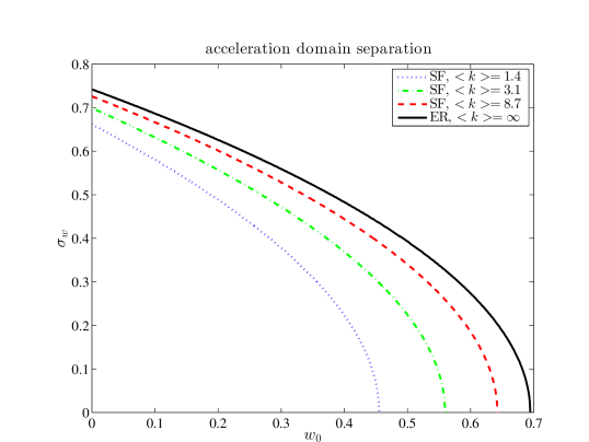
Figure 1: Acceleration domain boundaries for power-law graphs with $\left\langle k\right\rangle\simeq 1.4$ (blue, dotted), $\left\langle k\right\rangle\simeq 3.1$ (green, dash-dotted) and $\left\langle k\right\rangle\simeq 8.7$ (red,dashed), and the Erdös-Rényi graph with infinite connectivity (black, solid). The external domain (large $w_{0}$, large $\sigma_{w}$) has positive acceleration, marking a destabilizing effect of interactions.

4.2 Macro-economic sensitivity

The Basel regulatory framework (Basel II and III) requires banks to take into account cyclical effects and macro-economic factors in their risk estimate, in the shape of a countercyclical capital buffer. It is thus worthwhile to investigate the default probability across the economic cycle in our setting, highlighting once again the destabilizing effect of interactions. Assuming for simplicity that these cyclical effects to change slowly over the course of a year, we set $\xi_{0,t}=\xi_{0}$ in (7) to reflect macro-economic condition, and set $\xi_{0}$ to be a Gaussian r.v. (positive $\xi_{0}$ reflecting favorable, negative $\xi_{0}$ reflecting unfavorable conditions).

We can then study the distribution $P(\rho_{T})$ of the defaulted end-of-year fraction $\rho(T)$ induced by the distribution of $\xi_{0}$, the shape of the large $\rho(T)$-tail giving an indication as to the vulnerability of the system to large-scale economic shocks. This is done in figure 2, with an empirical distribution obtained from $10^{7}$ runs ($10^{3}$ runs on $10^{4}$ graphs). The non-interacting case is added for comparison.

As we can see the tail of the probability at large defaulted fraction $\rho$ is noticeably fatter in the presence of interactions, making the systemic risk much larger in bad macro-economic conditions, and suggests that correspondingly large buffers are needed.

Within the present study we have not specifically looked into the effects of pro-cyclical or countercyclical behavior of banks, although such effects could be included in our model. We refer to the concluding section for a discussion of these effects.

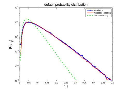
Figure 2: Default distribution for $\xi_{0}\sim\mathcal{N}\left(0,0.2\right)$: Simulations (blue dotted line) compared with cavity predictions (red solid line) and with the non-interacting network (green dashed line).

4.3 Interaction strength

In figure 3 we plot the time dependent defaulted fraction $\rho(t)$ at neutral macro-economic conditions ($\xi_{0,t}=0$) for different values of the interaction strength $w_{0}$. We set $\sigma_{w}$ to half the value of $w_{0}$, and average the simulation results over 250 graphs, with 500 runs on each graph.

As expected, the finite-size effects becomes larger as the interaction strength increases, which is to be expected: while the cavity method is exact on trees, the presence of loops strongly affects its performance. And while the graphs used are locally tree-like, for finite size systems there are still a large number of loops remaining. Since these loops only affect the dynamics when their constitutive nodes are defaulted, their effect is felt more strongly when the default rate is higher.

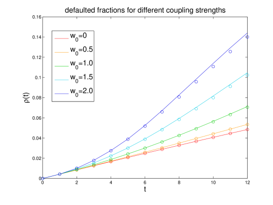
Figure 3: Defaulted fractions for different mean coupling strengths: simulation (circles) and cavity predictions (solid lines).

4.4 Extension: spillover

An important extension of the model is the inclusion of spillover effects, as induced by asset fire-sales. A fire-sale happens when a firm, short on liquidity, sells a large amount of assets in a short time (in the case of banks, it is a regulatory requirement to maintain a certain size of its liquid capital buffer). As a result of the sudden glut, asset prices will fall, diminishing the value of assets held by other firms.

To implement this, we consider for simplicity a single class $a$ of (tradable) assets, representing a given (constant) fraction of every firm’s wealth. When a firm’s wealth falls below a certain fraction $f_{c}$ of its initial wealth it enters a distressed state and sells asset $a$ to maintain liquidity, resulting in a fall of the asset price. As a result, the value of the portfolio of every firm holding this asset falls, which we model by changing the firms’ initial wealth by a factor $r(d_{t})=(1+r_{0}\,d_{t})^{-1}$ where $d_{t}$ is the fraction of distressed firms at time $t$ (defaulted firms are considered distressed as well), and $r_{0}$ a parameter that could describe market depth. Thus, a firm’s wealth at time $t$ becomes

$$\theta_{i,t}=r(d_{t-1})\,\theta_{i}-\sum_{\begin{subarray}{c}i\end{subarray}}w_{ij}c_{ij}n_{j,t}-\eta_{i,t}\ ,$$

and default is triggered when $\theta_{i,t}$ falls below zero, while the firm enters a distressed state as soon as $\theta_{i,t}<f_{c}\theta_{i}$.

This can be seen as implementing a simple version of the overlapping portfolio approach of [8] on top of the credit risk model, using in the present case only one asset class. Plotted below are the mean defaulted fraction in neutral macro-economic conditions ($\xi_{0}=0$, fig. 4(a)) and the probability distribution of defaulted fractions across the economic cycle as generated by a distribution of macro-economic conditions (fig. 4(b)), showing that spillover effects can dramatically increase the probability of large defaulted fractions. We take $f_{c}=0.1$.

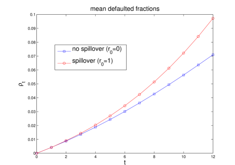
(a) Mean defaulted fractions under neutral macro-economic conditions ($\xi_{0}=0$) for a model with spillover $r_{0}=1$ (red circles) compared to results without spillover (blue squares).

these results

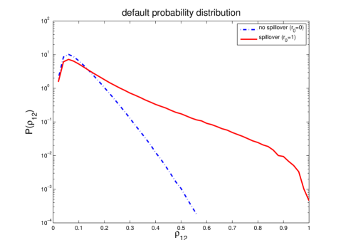
(b) End-of-year default probabilities with spillover $r_{0}=1$(red solid line) compared to results without spillover (blue dotted line) for $\xi_{0}\sim\mathcal{N}\left(0,0.2\right)$.

Figure 4:

While the network of exposures induced by assets is very different from the simple pairwise interaction network due to the inclusion of a bipartite (firms-assets) structure, as long as the number of asset classes remains finite in the large-system limit their contribution can be modeled by a simple mean-field effect as above. If the number of asset scales with $N$ however, the situation becomes much more complicated and depends on the details of the network structure and the interaction type.

4.5 Network size

To check the convergence of the simulation results towards cavity results valid in the thermodynamic limit $N\rightarrow\infty$, we plot the relative error of the defaulted fraction at $T=12$ compared to the cavity simulation $\epsilon=\tfrac{\left|\rho_{12}^{N}-\rho_{12}^{\infty}\right|}{\rho_{12}^{\infty}}$, for different network sizes. Numerical simulations are done on networks of size $N=200$ to $N=5000$. We average over 5000 graphs with 1000 runs on each graph (5000 runs for network sizes smaller than $10^{3}$). The results are plotted in figure 5. Since the variances of the cavity results are orders of magnitude smaller than those of the simulations, the error bars represent the RMSE of the simulations relative to the average cavity result, scaled by the square root of the number of simulation samples.

As expected, the finite-size simulations converge toward the message-passing solution with increasing $N$, and the quality of the approximation is in the 1% range even for $N$ as small as $N\simeq 10^{3}$. The convergence rate is compatible with an $N^{-1/2}$ law.

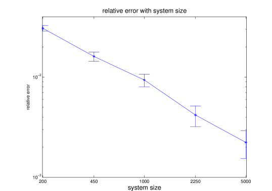
Figure 5: Log-log plot of the relative deviation of finite-size simulations from cavity predictions for different network sizes.

5 Conclusion

In this paper, we have studied the model of credit contagion introduced in [1], and have derived an analytic solution for the damage-spreading dynamics on generic locally tree-like sparse graphs in the thermodynamic limit, using both an adaptation of the method detailed in [32] and a generating functional analysis. While both approaches give rise to the same dynamical equations, the generating functional method opens up the perspective of developing systematic approximation schemes which could, for instance, provide simplified dynamic equations for the large mean connectivity limit, or allow a study of finite size corrections.

We have found the analytic predictions to be in good agreement with simulation results, both for average defaulted fractions and for distributions of end-of-year defaulted fractions induced by varying macro-economic conditions. This comparison of simulation results for moderate system sizes with results that would pertain to the thermodynamic limit, therefore, shows that the present theoretical approach does provide a viable description of contagion dynamics in large heterogeneous systems, even though finite instances will contain a fair amount of short loops.

Our preliminary results for a highly schematic scenario support the idea that spillover effects caused by asset fire-sales constitute a relevant driver of systemic instability, which appears to be at least as important as direct contagion. However, it would be interesting to investigate the contribution of large (scaling with $N$) numbers of assets in this model.

Our investigation of default distributions under varying macro-economic conditions shows strong risk enhancement in the absence of countercyclical measures. Our analysis could be expanded to investigate the effects of such measure, for example by considering $\xi_{0}$-dependent scalings of capital buffer sizes, exposure sizes (as given by interaction weights) or of initial wealth, or by combinations of these.

The method exposed here can easily be extended to more general models. In particular, it is straightforward to add recovery by including in our model a situation where upon default of node $i$ at time t, the loss incurred by its neighbors undergoes a damping of the type $w_{ji}(t+\tau)=r_{i}(\tau)w_{ji}$, where $r_{i}$ is chosen among a set of damping profiles (e.g. exponential damping, or a step function). In this case, we can make an easy parallel to the SIR model.

We believe our approach to be particularly suited to situations where detailed information is hard to come by, or where the network is so large as to make direct simulation unfeasible. Indeed, the message-passing scheme presented here does not depend on the network size.

On the analytical side, open questions remain. One question of interest is the computation of large-deviation functions, for which an annealed computation is possible using the current method but where quenched computations run into difficulties (e.g. we cannot, in the replica computation, factor the bond-disorder average).

6 Acknowledgements

This work has been supported by the People Programme (Marie Curie Actions) of the European Unions Seventh Frame- work Programme FP7/2007-2013/ under REA grant agreement n. 290038 (CF).

It is a pleasure to thank Luca Dall’Asta for enlightening discussions.

Appendix A Appendix

A.1 Generating Functional Analysis

We develop here the generating function analysis of the model described above. The analysis is very general and can be applied to almost any network where nodes are coupled via local fields. The method is well understood and has been used in a variety of other studies [36, 37, 38], although the version presented here differs in that instead of introducing a path integral, we can limit ourselves to a finite (low) number of integration parameters.

The method proceeds as follows: considering a particular degree sequence and wealth configuration, we introduce a generating function for the evaluation of averages and correlation functions of observables related to contagion dynamics as described by eq. (3) over the graph ensemble conditioned on the degree sequence. Taking advantage of the sparseness of the network, we express this generating function in terms of an integral with an effective action, and we compute the integral to order $N$ using a saddle-point approximation.

The initial part is simple: as is standard in field theory, we wish to compute a generating function for the correlations of observables $n_{i,t}$

$$G[\mbox{\boldmath$\psi$}|\mathbf{k}.\mbox{\boldmath$\theta$}]=\overline{\left\langle\exp\left\{\sum_{\begin{subarray}{c}i,t\end{subarray}}\psi_{i,t}n_{i,t}\right\}\right\rangle}$$ (16)

for a given auxiliary field $\psi$, where the $\left\langle\cdots\right\rangle$ denotes an average over the dynamics (the default times) for a given graph and wealth realization $(\mathbf{k},\mbox{\boldmath$\theta$})$, while $\overline{(\cdots)}$ denotes an average over the graphs compatible with this realization.

Once such a function has been computed, the average value $\overline{\left\langle n_{i,t}\right\rangle}$ can be obtained using

$$\overline{\left\langle n_{i,t}\right\rangle}=\left.\partial_{\psi_{i,t}}G[\mbox{\boldmath$\psi$}|\mathbf{k},\mbox{\boldmath$\theta$}]\right|_{\mbox{\boldmath$\psi$}=0}\ ,$$

while correlation functions are given by higher derivatives, such as

$$\overline{\left\langle n_{i,t}n_{j,t^{\prime}}\right\rangle}=\left.\partial_{\psi_{i,t}\psi_{j,t^{\prime}}}G[\mbox{\boldmath$\psi$}|\mathbf{k},\mbox{\boldmath$\theta$}]\right|_{\mbox{\boldmath$\psi$}=0}\ .$$

In our situation, we are primarily interested in the global average

$$\rho(t)=\dfrac{1}{N}\sum_{\begin{subarray}{c}i\end{subarray}}\overline{\left\langle n_{i,t}\right\rangle}\ .$$

Since we use the generating functional method only as a vehicle to obtain a macroscopic description of the dynamics, we can in fact drop the source fields $\psi_{i,t}$ entirely in what follows.

Carrying out the average over the graphs, i.e. over their adjacency matrix $\mathbf{A}$ and couplings $\mathbf{w}=\left\{w_{ij},w_{ji}\right\}_{(ij)}$, the generating function is expressed as

$$G[\mathbf{k},\mbox{\boldmath$\theta$}]=\sum_{\begin{subarray}{c}\mathbf{A}\end{subarray}}\int\mathrm{d}\mathbf{w}\,P(\mathbf{A},\mathbf{w}|\mathbf{k})\,\sum_{\begin{subarray}{c}\left\{t_{i}\right\}\end{subarray}}\prod_{\begin{subarray}{c}i\end{subarray}}P\left(t_{i}|\theta_{i},\mathbf{h}_{i}\right)\ .$$

We then use Dirac delta functions and their Fourier representations to ‘extract’ the dependence of the $P\left(t_{i}|\theta_{i},\mathbf{h}_{i}\right)$ on the couplings $\mathbf{w}$ via the local-fields $\{\mathbf{h}_{i}\}$ to obtain

$$G[\mathbf{k},\mbox{\boldmath$\theta$}]=\sum_{\begin{subarray}{c}\mathbf{A}\end{subarray}}\int\mathrm{d}\mathbf{w}\,P(\mathbf{A},\mathbf{w}|\mathbf{k})\,\int\prod_{\begin{subarray}{c}i\end{subarray}}\sum_{\begin{subarray}{c}t_{i}\end{subarray}}\int\dfrac{\mathrm{d}\mathbf{h}_{i}\,\mathrm{d}\mathbf{\hat{h}}_{i}\,}{(2\pi)^{T}}P\left(t_{i}|\theta_{i},\mathbf{h}_{i}\right)$$

$$\qquad\qquad\times\exp\left\{-i\mathbf{\hat{h}}_{i}\cdot\left(\mathbf{h}_{i}-\sum_{\begin{subarray}{c}j\end{subarray}}a_{ij}w_{ij}\mathbf{n}(t_{j})\right)\right\}\ ,$$ (17)

which, as we shall now see, allows the average over graphs to be performed.

A.2 Graph probabilities

When taking the average over graphs, even for tree-like graphs, we have a number of graph ensembles to choose from. They fall into two broad categories: micro-canonical ensembles, where adjacency matrices are drawn so as to exactly reproduce a given degree sequence (with a prescribed degree distribution), and canonical models where links are randomly chosen such that degrees follow a given degree sequence only on average.

In the following derivation, we use a micro-canonical configuration model: we consider a ”typical” (self-averaging) degree sequence $\mathbf{k}$, and we take a uniform probability on the graphs with this given degree sequence:

$$P(\mathbf{A},\mathbf{w}|\mathbf{k})\propto\prod_{\begin{subarray}{c}(ij)\end{subarray}}p_{w}(w_{ij},w_{ji})\delta_{a_{ij},a_{ji}}\prod_{\begin{subarray}{c}i\end{subarray}}\delta_{k_{i},\sum_{\begin{subarray}{c}j\end{subarray}}a_{ij}}\ .$$ (18)

It is easier for our purpose to rewrite it as

$$P(\mathbf{A},\mathbf{w}|\mathbf{k})\propto\prod_{\begin{subarray}{c}(ij)\end{subarray}}p_{w}(w_{ij},w_{ji})\delta_{a_{ij},a_{ji}}\left[\dfrac{\left\langle k\right\rangle}{N}\delta_{a_{ij},1}+\left(1-\dfrac{\left\langle k\right\rangle}{N}\right)\delta_{a_{ij},0}\right]\prod_{\begin{subarray}{c}i\end{subarray}}\delta_{k_{i},\sum_{\begin{subarray}{c}j\end{subarray}}a_{ij}}\ ,$$

where the extra factor is seen to be independent of the choice of $\mathbf{A}$ for all adjacency matrices compatible with the chosen degree sequence [36], allowing to absorb it in the overall normalization constant $\mathcal{N}$ of the distribution. We then use the Fourier decomposition of the Kronecker deltas to get

$$P(\mathbf{A},\mathbf{w}|\mathbf{k})=\dfrac{1}{\mathcal{N}}\int\prod_{\begin{subarray}{c}i\end{subarray}}\dfrac{\mathrm{d}\omega_{i}\,}{2\pi}e^{-i\omega_{i}k_{i}}\prod_{\begin{subarray}{c}(ij)\end{subarray}}p_{w}(w_{ij},w_{ji})\left[\dfrac{\left\langle k\right\rangle}{N}e^{i(\omega_{i}+\omega_{j})}\delta_{a_{ij},1}+\left(1-\dfrac{\left\langle k\right\rangle}{N}\right)\delta_{a_{ij},0}\right]\ .$$

The average over weighted graphs in eq. (A.1) factorizes with respect to the edges, so the generating function can be expressed as

$$G =\dfrac{1}{\mathcal{N}}\prod_{\begin{subarray}{c}i\end{subarray}}\sum_{\begin{subarray}{c}t_{i}\end{subarray}}\int\dfrac{\mathrm{d}\mathbf{h}_{i}\,\mathrm{d}\mathbf{\hat{h}}_{i}\,}{(2\pi)^{T}}\dfrac{\mathrm{d}\omega_{i}\,}{2\pi}e^{-i\omega_{i}k_{i}}P\left(t_{i}|\theta_{i},\mathbf{h}_{i}\right)e^{-i\mathbf{\hat{h}}_{i}\cdot\mathbf{h}_{i}}\prod_{\begin{subarray}{c}(ij)\end{subarray}}D_{ij}\ ,$$

in which the individual edge contributions $D_{ij}$ take the form

$$D_{ij}= \sum_{\begin{subarray}{c}a_{ij}=0,1\end{subarray}}\int\mathrm{d}w_{ij}\,\mathrm{d}w_{ji}\,p_{w}(w_{ij},w_{ji})\left[\dfrac{\left\langle k\right\rangle}{N}e^{i(\omega_{i}+\omega_{j})}\delta_{a_{ij},1}+\left(1-\dfrac{\left\langle k\right\rangle}{N}\right)\delta_{a_{ij},0}\right]$$

$$\times\exp\left\{a_{ij}\left[iw_{ij}\mathbf{\hat{h}}_{i}\cdot\mathbf{n}(t_{j})+iw_{ji}\mathbf{\hat{h}}_{j}\cdot\mathbf{n}(t_{i})\right]\right\}$$

$$= \int\mathrm{d}w_{ij}\,\mathrm{d}w_{ji}\,p_{w}(w_{ij},w_{ji})$$

$$\times\left\{1+\dfrac{\left\langle k\right\rangle}{N}\left[e^{i(\omega_{i}+\omega_{j})}\exp i\left\{w_{ij}\mathbf{\hat{h}}_{i}\cdot\mathbf{n}(t_{j})+w_{ji}\mathbf{\hat{h}}_{j}\cdot\mathbf{n}(t_{i})\right\}-1\right]\right\}\ .$$ (19)

We can carry out the integration over the edge weights, and as it turns out the integral is factorizable even if $p(w_{ij},w_{ji})$ is not:

$$\left\langle e^{iw_{ij}\mathbf{\hat{h}}_{i}\cdot\mathbf{n}(t_{j})}e^{iw_{ji}\mathbf{\hat{h}}_{j}\cdot\mathbf{n}(t_{i})}\right\rangle_{w_{ij},w_{ji}}=\left\langle e^{iw_{ij}\mathbf{\hat{h}}_{i}\cdot\mathbf{n}(t_{j})}\right\rangle_{w_{ij}}\left\langle e^{iw_{ji}\mathbf{\hat{h}}_{j}\cdot\mathbf{n}(t_{i})}\right\rangle_{w_{ji}}$$ (20)

It is intuitively clear why this should be the case: since a node once defaulted is not influenced by the subsequent defaults of its neighbors, the value of these couplings is irrelevant. Thus, if node $i$ defaults first, whether $w_{ji}$ follows the marginal distribution or the conditional $p(w_{ji}|w_{ij})$ is both irrelevant and impossible to determine, and we can assume the former.

From the formal point of view, this is due to a rather subtle point: for a given node $i$ with default time $t_{i}$, while the fields $\mathbf{h}_{i}$ and $\mathbf{\hat{h}}_{i}$ have $T$ components $(h_{i,0},h_{i,1},\cdots,h_{i,T-1})$, $P\left(t_{i}|\theta_{i},\mathbf{h}_{i}\right)$ only depends on the first $t_{i}-1$ components of $\mathbf{h}_{i}$. Therefore, for the remaining components, the integration over the $\left\{h_{i,s}\right\}_{s\geq t_{i}}$ yield $\delta(\hat{h}_{i,s})$. In order to avoid cluttering the expressions we do not carry out this integration explicitly, but note that $\hat{h}_{i,s}=0$ for $s\geq t_{i}$ implies

$$\exp i\left\{w_{ij}\mathbf{\hat{h}}_{i}\cdot\mathbf{n}(t_{j})+w_{ji}\mathbf{\hat{h}}_{j}\cdot\mathbf{n}(t_{i})\right\}=\exp i\left\{w_{ij}\sum_{\begin{subarray}{c}t_{j}\leq s<t_{i}\end{subarray}}\hat{h}_{i,s}+w_{ji}\sum_{\begin{subarray}{c}t_{i}\leq s<t_{j}\end{subarray}}\hat{h}_{j,s}\right\}\ ,$$

and thus only one among the pair $(w_{ij},w_{ji})$ appears in the integral. This “dynamical factorization” is a crucial simplification. To simplify our expressions, we introduce

$$\chi(\mathbf{\hat{h}},t)=\left\langle e^{iw\mathbf{\hat{h}}\cdot\mathbf{n}(t)}\right\rangle_{w}\ .$$ (21)

A.3 Effective action

Combining averages over all edge-related parts, we obtain

$$\prod_{\begin{subarray}{c}(ij)\end{subarray}}D_{ij}=\prod_{\begin{subarray}{c}(ij)\end{subarray}}\left(1+\dfrac{\left\langle k\right\rangle}{N}\left[\chi(\mathbf{\hat{h}}_{i},t_{j})\chi(\mathbf{\hat{h}}_{j},t_{i})e^{i(\omega_{i}+\omega_{j})}-1\right]\right)\ .$$

Assuming the graph to be sparse, i.e. $\left\langle k\right\rangle\ll N$, this can be rewritten in exponential form

$$\prod_{\begin{subarray}{c}(ij)\end{subarray}}D_{ij}= \exp\left\{\dfrac{\left\langle k\right\rangle}{N}\sum_{\begin{subarray}{c}(ij)\end{subarray}}\left[\chi(\mathbf{\hat{h}}_{i},t_{j})\chi(\mathbf{\hat{h}}_{j},t_{i})e^{i(\omega_{i}+\omega_{j})}-1\right]\right\}$$

$$= \exp\left\{\dfrac{\left\langle k\right\rangle}{2N}\sum_{\begin{subarray}{c}i,j\end{subarray}}\chi(\mathbf{\hat{h}}_{i},t_{j})\chi(\mathbf{\hat{h}}_{j},t_{i})e^{i(\omega_{i}+\omega_{j})}-\dfrac{N\left\langle k\right\rangle}{2}\right\}\ .$$ (22)

We shall absorb the $\tfrac{N\left\langle k\right\rangle}{2}$ part into the normalization constant $\mathcal{N}$. Writing

$$P(\omega,t,\mathbf{\hat{h}})=\dfrac{1}{N}\sum_{\begin{subarray}{c}i\end{subarray}}\delta(\omega-\omega_{i})\delta_{t,t_{i}}\delta(\mathbf{\hat{h}}-\mathbf{\hat{h}}_{i})\,$$

we can rewrite our previous expression (A.3) as

$$\prod_{\begin{subarray}{c}(ij)\end{subarray}}D_{ij}=\exp\left\{N\dfrac{\left\langle k\right\rangle}{2}\sum_{\begin{subarray}{c}t,t^{\prime}\end{subarray}}\int\mathrm{d}\mathbf{\hat{h}}\,\mathrm{d}\mathbf{\hat{h}}^{\prime}\,\int\mathrm{d}\omega\,\mathrm{d}\omega^{\prime}\,\chi(\mathbf{\hat{h}},t^{\prime})\chi(\mathbf{\hat{h}}^{\prime},t)e^{i\omega}e^{i\omega^{\prime}}P(\omega,t,\mathbf{\hat{h}})P(\omega^{\prime},t^{\prime},\mathbf{\hat{h}}^{\prime})\right\}\ .$$

We see that this form almost factorizes. We then introduce the quantity

$$m(t|t^{\prime})= \int\mathrm{d}\mathbf{\hat{h}}\,\mathrm{d}\omega\,\chi(\mathbf{\hat{h}},t^{\prime})e^{i\omega}P(\omega,t,\mathbf{\hat{h}})$$

$$= \int\mathrm{d}\mathbf{\hat{h}}\,\mathrm{d}\omega\,\dfrac{1}{N}\sum_{\begin{subarray}{c}i\end{subarray}}\delta(\omega-\omega_{i})\delta_{t,t_{i}}\delta(\mathbf{\hat{h}}-\mathbf{\hat{h}}_{i})\chi(\mathbf{\hat{h}},t^{\prime})e^{i\omega}$$

$$= \dfrac{1}{N}\sum_{\begin{subarray}{c}i\end{subarray}}\delta_{t,t_{i}}\chi(\mathbf{\hat{h}}_{i},t^{\prime})e^{i\omega_{i}}\ ,$$

and decouple the sites by considering the $m(t|t^{\prime})$ as integration variables, using auxiliary variables $\hat{m}(t|t^{\prime})$ to enforce their definition via Fourier representations of $\delta$-functions:

$$1=\int\dfrac{\mathrm{d}m(t|t^{\prime})\,\mathrm{d}\hat{m}(t|t^{\prime})\,}{2\pi/N}\exp\left\{-i\hat{m}(t|t^{\prime})\left(Nm(t|t^{\prime})-\sum_{\begin{subarray}{c}i\end{subarray}}\delta_{t,t_{i}}\chi(\mathbf{\hat{h}}_{i},t^{\prime})e^{i\omega_{i}}\right)\right\}\ .$$

We notice that after the introduction of this integral, sites are effectively decoupled. As a result the generating function reads, to leading order in $N$,

$$G=\dfrac{1}{\mathcal{N}}\int\prod_{\begin{subarray}{c}t,t^{\prime}\end{subarray}}\dfrac{\mathrm{d}m(t|t^{\prime})\,\mathrm{d}\hat{m}(t|t^{\prime})\,}{2\pi/N}\exp\left\{N\left[G_{1}+G_{2}+G_{3}\right]\right\}\ ,$$

with

$$G_{1}= \dfrac{\left\langle k\right\rangle}{2}\sum_{\begin{subarray}{c}t,t^{\prime}\end{subarray}}m(t|t^{\prime})m(t^{\prime}|t)\ ,$$

$$G_{2}= -i\sum_{\begin{subarray}{c}t,t^{\prime}\end{subarray}}m(t|t^{\prime})\hat{m}(t|t^{\prime})\ ,$$

$$G_{3}= \dfrac{1}{N}\sum_{\begin{subarray}{c}i\end{subarray}}\ln Z_{i}\ ,$$

where

$$Z_{i}= \sum_{\begin{subarray}{c}t\end{subarray}}\int\dfrac{\mathrm{d}\mathbf{h}\,\mathrm{d}\mathbf{\hat{h}}\,}{(2\pi)^{T}}\dfrac{\mathrm{d}\omega\,}{2\pi}e^{-i\omega k_{i}}P\left(t|\theta_{i},\mathbf{h}\right)e^{-i\mathbf{\hat{h}}\cdot\mathbf{h}}\exp\left\{ie^{i\omega}\sum_{\begin{subarray}{c}t^{\prime}\end{subarray}}\chi(\mathbf{\hat{h}},t^{\prime})\hat{m}(t|t^{\prime})\right\}\ .$$ (23)

Using the self-averaging properties of the $(\mathbf{k},\theta)$ configuration, we can replace $\tfrac{1}{N}\sum_{i}Z_{i}(k_{i},\theta_{i})$ with $\left\langle Z(k,\theta)\right\rangle_{k,\theta}$ while only making an error of order $N^{-1/2}$. The function $G=G_{1}+G_{2}+G_{3}$ is the effective action of the problem.

A.4 Saddle-point

Now, considering the form of the integral, we are led in the $N\rightarrow\infty$ limit to consider a saddle-point approximation, which will lead us to replace to leading order the integral by its value at the saddle-point. The saddle-point equations

$$\dfrac{\partial}{\partial m(t|t^{\prime})}\left(G_{1}+G_{2}+G_{3}\right)=0$$

and

$$\dfrac{\partial}{\partial\hat{m}(t|t^{\prime})}\left(G_{1}+G_{2}+G_{3}\right)=0$$

read

$$\left\langle k\right\rangle m(t^{\prime}|t)=i\hat{m}(t|t^{\prime})$$ (24)

and

$$m(t|t^{\prime})=$$

$$\mathopen{\leavevmode\resizebox{1.2pt}{32.10852pt}{\Bigg{\langle}}}\leavevmode\hbox{$\dfrac{\int\frac{\mathrm{d}\mathbf{h}\,\mathrm{d}\mathbf{\hat{h}}\,}{(2\pi)^{T}}\int\frac{\mathrm{d}\omega\,}{2\pi}P\left(t|\theta,\mathbf{h}\right)e^{-i\mathbf{\hat{h}}\cdot\mathbf{h}}e^{-i\omega(k-1)}\chi(\mathbf{\hat{h}},t^{\prime})\exp\left\{ie^{i\omega}\sum_{\begin{subarray}{c}t^{\prime}\end{subarray}}\chi(\mathbf{\hat{h}},t^{\prime})\hat{m}(t|t^{\prime})\right\}}{\sum_{\begin{subarray}{c}s\end{subarray}}\frac{\mathrm{d}\mathbf{h}\,\mathrm{d}\mathbf{\hat{h}}\,}{(2\pi)^{T}}\int\frac{\mathrm{d}\omega\,}{2\pi}P\left(s|\theta,\mathbf{h}\right)e^{-i\mathbf{\hat{h}}\cdot\mathbf{h}}e^{-i\omega k}\exp\left\{ie^{i\omega}\sum_{\begin{subarray}{c}s^{\prime}\end{subarray}}\chi(\mathbf{\hat{h}},s^{\prime})\hat{m}(s|s^{\prime})\right\}}$}\mathclose{\leavevmode\resizebox{1.2pt}{32.10852pt}{\Bigg{\rangle}}_{k,\theta}}\ .$$

We can carry out the integration over $\omega$, and using (24), this gives

$$m(t|t^{\prime})=$$

$$\mathopen{\leavevmode\resizebox{1.2pt}{32.10852pt}{\Bigg{\langle}}}\leavevmode\hbox{$\sum_{\begin{subarray}{c}k\end{subarray}}\dfrac{kp_{k}}{\left\langle k\right\rangle}\dfrac{\int\frac{\mathrm{d}\mathbf{h}\,\mathrm{d}\mathbf{\hat{h}}\,}{(2\pi)^{T}}P\left(t|\theta,\mathbf{h}\right)e^{-i\mathbf{\hat{h}}\cdot\mathbf{h}}\chi(\mathbf{\hat{h}},t^{\prime})\left\{\sum_{\begin{subarray}{c}t^{\prime}\end{subarray}}\chi(\mathbf{\hat{h}},t^{\prime})m(t^{\prime}|t)\right\}^{k-1}}{\sum_{\begin{subarray}{c}s\end{subarray}}\int\frac{\mathrm{d}\mathbf{h}\,\mathrm{d}\mathbf{\hat{h}}\,}{(2\pi)^{T}}P\left(s|\theta,\mathbf{h}\right)e^{-i\mathbf{\hat{h}}\cdot\mathbf{h}}\left\{\sum_{\begin{subarray}{c}s^{\prime}\end{subarray}}\chi(\mathbf{\hat{h}},s^{\prime})m(s^{\prime}|s)\right\}^{k}}$}\mathclose{\leavevmode\resizebox{1.2pt}{32.10852pt}{\Bigg{\rangle}}_{\theta}}\ .$$ (25)

We can interpret the $m(t|t^{\prime})$ using the same method as in [36]: the $m(t|t^{\prime})$ at the saddle-point appear as conditional probabilities, i.e. the probability that a node default at time $t$ given that we know one of its neighbors has defaulted at time $t^{\prime}$. Thus we must have $\sum_{t}m(t|t^{\prime})=1$, remembering that we are also considering in this sum the probability that the node has not defaulted within the finite risk horizon, $1,\dots,T$.

Another way of looking at things is that we assume the normalization $\sum_{t}m(t|t^{\prime})=1$ and will show that such solutions are self-consistent and coincide with the messages introduced in the message-passing solution.

We now remember two things. First, in the integral in the numerator of (A.4) all components $\hat{h}_{s}$ for $s\geq t$ cancel, as was noted previously and exploited in eq. (20). Second, $\chi(\mathbf{\hat{h}},t^{\prime})$ is a function of the scalar product $\mathbf{\hat{h}}\cdot\mathbf{n}(t^{\prime})=\sum_{s=t^{\prime}}^{T-1}\hat{h}_{s}$. Therefore in the integral in (A.4) this sum is actually $\mathbf{\hat{h}}\cdot\mathbf{n}(t^{\prime})=\sum_{s=t^{\prime}}^{t-1}\hat{h}_{s}$, and therefore $\chi(\mathbf{\hat{h}},t^{\prime}\geq t)=\chi(0,t^{\prime})=1$.

Consequently $m(t|s\geq t)=m(t|t)$, e.g. for example $m(1|2)=m(1|1)$. This is clear from the interpretation of the $m(t|t^{\prime})$ given above, since defaults of a neighbor after one’s own default cannot influence the original node as was noted in previous sections. We thus write, as previously in section 3, $m(t)\equiv m(t|t^{\prime}\geq t)$.

Using these observations, we can simplify our equations further. First we notice that with these conventions, in eq. (A.4) we have

$$\sum_{\begin{subarray}{c}t^{\prime}\end{subarray}}\chi(\mathbf{\hat{h}},t^{\prime})m(t^{\prime}|t)=\left(1-\sum_{\begin{subarray}{c}t^{\prime}<t\end{subarray}}m(t^{\prime})\right)+\sum_{\begin{subarray}{c}t^{\prime}<t\end{subarray}}m(t^{\prime})\chi(\mathbf{\hat{h}},t^{\prime})\ ,$$

since, as was previously noted, all the components $\hat{h}_{s}$ vanish for $s\geq t$ and $\chi\left(\mathbf{\hat{h}},t^{\prime}\right)$ only depends on the components $\hat{h}_{s}$ for $s\geq t^{\prime}$.

Second, we notice that the denominator

$$\sum_{\begin{subarray}{c}s\end{subarray}}\int\frac{\mathrm{d}\mathbf{h}\,\mathrm{d}\mathbf{\hat{h}}\,}{(2\pi)^{T}}P\left(s|\theta,\mathbf{h}\right)e^{-i\mathbf{\hat{h}}\cdot\mathbf{h}}\left\{\sum_{\begin{subarray}{c}s^{\prime}\end{subarray}}\chi(\mathbf{\hat{h}},s^{\prime})m(s^{\prime}|s)\right\}^{k}$$

in (A.4) is equal to 1.

Indeed, consider the simple situation where $T=2$: we have three possible trajectories:

• a node defaults on the first time step ($t=1$), corresponding to the term

  $$\int\frac{\mathrm{d}\mathbf{h}\,\mathrm{d}\mathbf{\hat{h}}\,}{(2\pi)^{2}}W_{0}(-\theta)e^{-i\mathbf{\hat{h}}\cdot\mathbf{h}}=W_{0}(-\theta)$$

  in the denominator

• a node defaults on the second time step ($t=2$), to which corresponds the term

  $$\int\frac{\mathrm{d}\mathbf{h}\,\mathrm{d}\mathbf{\hat{h}}\,}{(2\pi)^{2}}\left(1-W_{0}(-\theta)\right)W_{1}(h_{1}-\theta)e^{-i\mathbf{\hat{h}}\cdot\mathbf{h}}\left\{m(1)\chi(\mathbf{\hat{h}},1)+\left(1-m(1)\right)\right\}^{k}$$

• a node does not default during the time horizon, to which corresponds the term

  $$\int\frac{\mathrm{d}\mathbf{h}\,\mathrm{d}\mathbf{\hat{h}}\,}{(2\pi)^{2}}\left(1-W_{0}(-\theta)\right)\left(1-W_{1}(h_{1}-\theta)\right)e^{-i\mathbf{\hat{h}}\cdot\mathbf{h}}\left\{m(1)\chi(\mathbf{\hat{h}},1)+\left(1-m(1)\right)\right\}^{k}$$

  as in eq. (6)

Summing these terms, we find

$$Z(k,\theta)= W_{0}(-\theta)+\int\frac{\mathrm{d}\mathbf{h}\,\mathrm{d}\mathbf{\hat{h}}\,}{(2\pi)^{2}}\left(1-W_{0}(-\theta)\right)W_{1}(h_{1}-\theta)e^{-i\mathbf{\hat{h}}\cdot\mathbf{h}}\left\{m(1)\chi(\mathbf{\hat{h}},1)+\left(1-m(1)\right)\right\}^{k}$$

$$+\int\frac{\mathrm{d}\mathbf{h}\,\mathrm{d}\mathbf{\hat{h}}\,}{(2\pi)^{2}}\left(1-W_{0}(-\theta)\right)\left(1-W_{1}(h_{1}-\theta)\right)e^{-i\mathbf{\hat{h}}\cdot\mathbf{h}}\left\{m(1)\chi(\mathbf{\hat{h}},1)+\left(1-m(1)\right)\right\}^{k}$$

$$= W_{0}(-\theta)+\int\frac{\mathrm{d}\mathbf{h}\,\mathrm{d}\mathbf{\hat{h}}\,}{(2\pi)^{2}}\left(1-W_{0}(-\theta)\right)e^{-i\mathbf{\hat{h}}\cdot\mathbf{h}}\left\{m(1)\chi(\mathbf{\hat{h}},1)+\left(1-m(1)\right)\right\}^{k}$$

$$= W_{0}(-\theta)+\left(1-W_{0}(-\theta)\right)=1\ ,$$

and the reasoning can be extended without major difficulty to $T>2$.

Finally, the saddle-point equations for the quantities $m(t|t^{\prime})$ read

$$m(t|t^{\prime})=$$

$$\left\langle\sum_{\begin{subarray}{c}k\end{subarray}}\dfrac{kp_{k}}{\left\langle k\right\rangle}\int\frac{\mathrm{d}\mathbf{h}\,\mathrm{d}\mathbf{\hat{h}}\,}{(2\pi)^{T}}P\left(t|\theta,\mathbf{h}\right)e^{-i\mathbf{\hat{h}}\cdot\mathbf{h}}\chi(\mathbf{\hat{h}},t^{\prime})\left\{\sum_{\begin{subarray}{c}t^{\prime\prime}<t\end{subarray}}m(t^{\prime\prime})\chi(\mathbf{\hat{h}},t^{\prime\prime})+\left(1-\sum_{\begin{subarray}{c}t^{\prime\prime}<t\end{subarray}}m(t^{\prime\prime})\right)\right\}^{k-1}\right\rangle_{\theta}\ ,$$

while

$$m(t)=$$

$$\left\langle\sum_{\begin{subarray}{c}k\end{subarray}}\dfrac{kp_{k}}{\left\langle k\right\rangle}\int\frac{\mathrm{d}\mathbf{h}\,\mathrm{d}\mathbf{\hat{h}}\,}{(2\pi)^{T}}P\left(t|\theta,\mathbf{h}\right)e^{-i\mathbf{\hat{h}}\cdot\mathbf{h}}\left\{\sum_{\begin{subarray}{c}t^{\prime}<t\end{subarray}}m(t^{\prime})\chi(\mathbf{\hat{h}},t^{\prime})+\left(1-\sum_{\begin{subarray}{c}t^{\prime}<t\end{subarray}}m(t^{\prime})\right)\right\}^{k-1}\right\rangle_{\theta}\ .$$ (26)

The (average) default probabilities are given by

$$p(t)=$$

$$\left\langle\int\frac{\mathrm{d}\mathbf{h}\,\mathrm{d}\mathbf{\hat{h}}\,}{(2\pi)^{T}}P\left(t|\theta,\mathbf{h}\right)e^{-i\mathbf{\hat{h}}\cdot\mathbf{h}}\left\{\sum_{\begin{subarray}{c}t^{\prime}<t\end{subarray}}m(t^{\prime})\chi(\mathbf{\hat{h}},t^{\prime})+\left(1-\sum_{\begin{subarray}{c}t^{\prime}<t\end{subarray}}m(t^{\prime})\right)\right\}^{k}\right\rangle_{k,\theta}\ .$$

What is the connection between these equations and their message-passing equivalents ? Recall that

$$\chi(\mathbf{\hat{h}},t)=\left\langle e^{iw\mathbf{\hat{h}}\cdot\mathbf{n}(t)}\right\rangle_{w}\ .$$

Thus upon expanding (A.4), we obtain

$$m(t)= \left\langle\sum_{\begin{subarray}{c}k\end{subarray}}\dfrac{kp_{k}}{\left\langle k\right\rangle}\int\frac{\mathrm{d}\mathbf{h}\,\mathrm{d}\mathbf{\hat{h}}\,}{(2\pi)^{T}}P\left(t|\theta,\mathbf{h}\right)e^{-i\mathbf{\hat{h}}\cdot\mathbf{h}}\sum_{\begin{subarray}{c}q=0\end{subarray}}^{k-1}\binom{k-1}{q}\left(1-\sum_{\begin{subarray}{c}t^{\prime}<t\end{subarray}}m(t^{\prime})\right)^{k-q}\right.$$

$$\left.\quad\times\sum_{\begin{subarray}{c}\tau_{1},\cdots,\tau_{q}<t\end{subarray}}\prod_{\begin{subarray}{c}i=1\end{subarray}}^{q}\chi(\mathbf{\hat{h}},t_{i})m(\tau_{i})\right\rangle_{\theta}$$

$$= \left\langle\sum_{\begin{subarray}{c}k\end{subarray}}\dfrac{kp_{k}}{\left\langle k\right\rangle}\int\frac{\mathrm{d}\mathbf{h}\,\mathrm{d}\mathbf{\hat{h}}\,}{(2\pi)^{T}}P\left(t|\theta,\mathbf{h}\right)e^{-i\mathbf{\hat{h}}\cdot\mathbf{h}}\sum_{\begin{subarray}{c}q=0\end{subarray}}^{k-1}\binom{k-1}{q}\left(1-\sum_{\begin{subarray}{c}t^{\prime}<t\end{subarray}}m(t^{\prime})\right)^{k-1-q}\right.$$

$$\left.\quad\times\sum_{\begin{subarray}{c}\tau_{1},\cdots,\tau_{q}<t\end{subarray}}\int\prod_{\begin{subarray}{c}i=1\end{subarray}}^{q}\mathrm{d}w_{i}\,p_{w}(w_{i})m(\tau_{i})e^{iw_{i}\mathbf{\hat{h}}\cdot\mathbf{n}(\tau_{i})}\right\rangle_{\theta}$$

$$= \left\langle\sum_{\begin{subarray}{c}k\end{subarray}}\dfrac{kp_{k}}{\left\langle k\right\rangle}\int\mathrm{d}\mathbf{h}\,P\left(t|\theta,\mathbf{h}\right)\sum_{\begin{subarray}{c}q=0\end{subarray}}^{k-1}\binom{k-1}{q}\left(1-\sum_{\begin{subarray}{c}t^{\prime}<t\end{subarray}}m(t^{\prime})\right)^{k-1-q}\right.$$

$$\left.\quad\times\sum_{\begin{subarray}{c}\tau_{1},\cdots,\tau_{q}<t\end{subarray}}\int\prod_{\begin{subarray}{c}i=1\end{subarray}}^{q}\mathrm{d}w_{i}\,p_{w}(w_{i})m(\tau_{i})\delta(\mathbf{h}-\sum_{\begin{subarray}{c}i=1\end{subarray}}^{q}w_{i}\mathbf{n}(\tau_{i}))\right\rangle_{\theta}$$

$$= \sum_{\begin{subarray}{c}k\end{subarray}}\dfrac{kp_{k}}{\left\langle k\right\rangle}\sum_{\begin{subarray}{c}q=0\end{subarray}}^{k-1}\binom{k-1}{q}\left(1-\sum_{\begin{subarray}{c}t^{\prime}<t\end{subarray}}m(t^{\prime})\right)^{k-1-q}$$

$$\quad\times\sum_{\begin{subarray}{c}\tau_{1},\cdots,\tau_{q}<t\end{subarray}}\int\prod_{\begin{subarray}{c}i=1\end{subarray}}^{q}\mathrm{d}w_{i}\,p_{w}(w_{i})m(\tau_{i})\left\langle P\left(t|\theta,\sum_{\begin{subarray}{c}i=1\end{subarray}}^{q}w_{i}\mathbf{n}(\tau_{i})\right)\right\rangle_{\theta}\ ,$$

which can be seen to be the same as (13).

References

- [1] J. Hatchett and R. Kühn, “Effects of economic interactions on credit risk,” Journal of Physics A: Mathematical and General, vol. 39, no. 10, p. 2231, 2006.
- [2] B. Karrer and M. E. Newman, “Message passing approach for general epidemic models,” Physical Review E, vol. 82, no. 1, p. 016101, 2010.
- [3] A. G. Haldane and R. M. May, “Systemic risk in banking ecosystems,” Nature, vol. 469, no. 7330, pp. 351–355, 2011.
- [4] R. C. Merton, “On the pricing of corporate debt: The risk structure of interest rates*,” The Journal of Finance, vol. 29, no. 2, pp. 449–470, 1974.
- [5] P. Gai and S. Kapadia, “Contagion in financial networks,” Proceedings of the Royal Society A: Mathematical, Physical and Engineering Science, vol. 466, no. 2120, pp. 2401–2423, 2010.
- [6] D. Egloff, M. Leippold, and P. Vanini, “A simple model of credit contagion,” Journal of Banking & Finance, vol. 31, no. 8, pp. 2475–2492, 2007.
- [7] S. Heise and R. Kühn, “Derivatives and credit contagion in interconnected networks,” The European Physical Journal B, vol. 85, no. 4, pp. 1–19, 2012.
- [8] F. Caccioli, M. Shrestha, C. Moore, and J. D. Farmer, “Stability analysis of financial contagion due to overlapping portfolios,” Journal of Banking & Finance, 2014.
- [9] R. M. May and N. Arinaminpathy, “Systemic risk: the dynamics of model banking systems,” Journal of the Royal Society Interface, vol. 7, no. 46, pp. 823–838, 2010.
- [10] D. Lando, “On cox processes and credit risky securities,” Review of Derivatives research, vol. 2, no. 2-3, pp. 99–120, 1998.
- [11] D. Duffie and K. J. Singleton, “Modeling term structures of defaultable bonds,” Review of Financial studies, vol. 12, no. 4, pp. 687–720, 1999.
- [12] A. Elizalde, “Credit risk models ii: Structural models,” Available on www. defaultrisk. com/pp model, vol. 86, 2005.
- [13] S. N. Durlauf, “Statistical mechanics approaches to socioeconomic behavior,” 1996.
- [14] J.-P. Bouchaud, “Crises and collective socio-economic phenomena: simple models and challenges,” Journal of Statistical Physics, vol. 151, no. 3-4, pp. 567–606, 2013.
- [15] F. Liljeros, C. R. Edling, L. A. N. Amaral, H. E. Stanley, and Y. Åberg, “The web of human sexual contacts,” Nature, vol. 411, no. 6840, pp. 907–908, 2001.
- [16] A. Vázquez, “Statistics of citation networks,” arXiv preprint cond-mat/0105031, 2001.
- [17] L. A. Adamic and B. A. Huberman, “Power-law distribution of the world wide web,” Science, vol. 287, no. 5461, pp. 2115–2115, 2000.
- [18] P. Crucitti, V. Latora, and M. Marchiori, “A topological analysis of the italian electric power grid,” Physica A: Statistical Mechanics and its Applications, vol. 338, no. 1, pp. 92–97, 2004.
- [19] A.-L. Barabási and R. Albert, “Emergence of scaling in random networks,” Science, vol. 286, no. 5439, pp. 509–512, 1999.
- [20] F. Caccioli, T. A. Catanach, and J. D. Farmer, “Heterogeneity, correlations and financial contagion,” Advances in Complex Systems (ACS), vol. 15, 2012.
- [21] M. E. Newman, “Spread of epidemic disease on networks,” Physical review E, vol. 66, no. 1, p. 016128, 2002.
- [22] C. Moore and M. E. Newman, “Epidemics and percolation in small-world networks,” Physical Review E, vol. 61, no. 5, p. 5678, 2000.
- [23] M. Mezard and A. Montanari, Information, physics, and computation. Oxford University Press, 2009.
- [24] M. Mézard and G. Parisi, “The bethe lattice spin glass revisited,” The European Physical Journal B-Condensed Matter and Complex Systems, vol. 20, no. 2, pp. 217–233, 2001.
- [25] F. Altarelli, A. Braunstein, L. Dall’Asta, J. Wakeling, and R. Zecchina, “Containing epidemic outbreaks by message-passing techniques,” Physical Review X, vol. 4, no. 2, p. 021024, 2014.
- [26] F. Caccioli, J. D. Farmer, N. Foti, and D. Rockmore, “How interbank lending amplifies overlapping portfolio contagion: A case study of the austrian banking network,” arXiv preprint arXiv:1306.3704, 2013.
- [27] W. Souma, Y. Fujiwara, and H. Aoyama, “Complex networks and economics,” Physica A: Statistical Mechanics and its Applications, vol. 324, no. 1, pp. 396–401, 2003.
- [28] D. Centola and M. Macy, “Complex contagions and the weakness of long ties,” American Journal of Sociology, vol. 113, no. 3, pp. 702–734, 2007.
- [29] D. J. Watts, “A simple model of global cascades on random networks,” Proceedings of the National Academy of Sciences, vol. 99, no. 9, pp. 5766–5771, 2002.
- [30] F. Caccioli, J. D. Farmer, N. Foti, and D. Rockmore, “Overlapping portfolios, contagion, and financial stability,” Journal of Economic Dynamics and Control, 2014.
- [31] Basel II, “International convergence of capital measurement and capital standards: a revised framework,” 2006.
- [32] A. Y. Lokhov, M. Mézard, and L. Zdeborová, “Dynamic message-passing equations for models with unidirectional dynamics,” arXiv preprint arXiv:1407.1255, 2014.
- [33] H. Ohta and S.-i. Sasa, “A universal form of slow dynamics in zero-temperature random-field ising model,” EPL (Europhysics Letters), vol. 90, no. 2, p. 27008, 2010.
- [34] F. Altarelli, A. Braunstein, L. Dall’Asta, and R. Zecchina, “Large deviations of cascade processes on graphs,” Physical Review E, vol. 87, no. 6, p. 062115, 2013.
- [35] A. Y. Lokhov, M. Mézard, H. Ohta, and L. Zdeborová, “Inferring the origin of an epidemic with a dynamic message-passing algorithm,” Phys. Rev. E, vol. 90, p. 012801, Jul 2014.
- [36] K. Mimura and A. Coolen, “Parallel dynamics of disordered ising spin systems on finitely connected directed random graphs with arbitrary degree distributions,” Journal of Physics A: Mathematical and Theoretical, vol. 42, no. 41, p. 415001, 2009.
- [37] A. Coolen and S. Rabello, “Generating functional analysis of complex formation and dissociation in large protein interaction networks,” in Journal of Physics: Conference Series, vol. 197, p. 012006, IOP Publishing, 2009.
- [38] J. Hatchett, B. Wemmenhove, I. P. Castillo, T. Nikoletopoulos, N. Skantzos, and A. Coolen, “Parallel dynamics of disordered ising spin systems on finitely connected random graphs,” Journal of Physics A: Mathematical and General, vol. 37, no. 24, p. 6201, 2004.