Cosmological dynamics in higher-dimensional Einstein-Gauss-Bonnet gravity

Abstract

In this paper we perform a systematic classification of the regimes of cosmological dynamics in Einstein-Gauss-Bonnet gravity with generic values of the coupling constants. We consider a manifold which is a warped product of a four dimensional Friedmann-Robertson-Walker space-time with a $D$-dimensional Euclidean compact constant curvature space with two independent scale factors. A numerical analysis of the time evolution as function of the coupling constants and of the curvatures of the spatial section and of the extra dimension is performed. We describe the distribution of the regimes over the initial conditions space and the coupling constants. The analysis is performed for two values of the number of extra dimensions ($D\geqslant 6$ both) which allows us to describe the effect of the number of the extra dimensions as well.

I Introduction

The action principle for General Relativity in four dimensions can be formulated by requiring that it should be constructed out of curvature invariants and that its variation should lead to second order field equations for the metric. Indeed in four dimensional space-time it can be easily shown that the only action that satisfies these two requirements is the Einstein-Hilbert action plus a cosmological term. Rigorously speaking one can add to the gravitational action also a Gauss-Bonnet term $\int\sqrt{-g}(R_{\mu\nu\alpha\beta}R^{\mu\nu\alpha\beta}-4R_{\mu\nu}R^{\mu\nu}+R^{2})$ as its variation does not affect the equations of motion being just a boundary term. This is only true in four dimensions as in five or higher dimensions the variation of the Gauss-Bonnet term gives a non-trivial contribution to the equations of motion which however remains of second order in the derivatives of the metric. In seven dimensions one can add another term to the gravitational action which is constructed from cubic curvature invariants and whose variation is again of second order in the metric. More generally in an $N$-dimensional space-time it is possible to construct an action which is the sum of $[\frac{N+1}{2}]$ independent terms which are of up to the $[\frac{N}{2}]$th power in the curvature and whose variation gives second order field equations for the metric. This gravity theory is known as Lovelock gravity Lovelock , and it is the most straightforward extension of General Relativity to higher dimensions as it is constructed according to the same principles as used for four dimensional General Relativity.

Einstein-Gauss-Bonnet (EGB) gravity is the most simple non-trivial example of Lovelock gravity and its action is the sum of a volume term $\int\sqrt{-g}$ an Einstein-Hilbert term $\int\sqrt{-g}R$and the Gauss-Bonnet term $\int\sqrt{-g}(R_{\mu\nu\alpha\beta}R^{\mu\nu\alpha\beta}-4R_{\mu\nu}R^{\mu\nu}+R^{2})$, each term having its own coupling constant. The reason why this action has attracted a lot of interest in theoretical physics is also because the low energy limit of some string theories (see, for instance, the discussion in GastGarr ) is described by Einstein-Gauss-Bonnet gravity rather then General Relativity. Actually the idea that space-time may have more than four dimensions is much older than string theory as it was already proposed by Kaluza KK1 and Klein KK2 ; KK3 in an attempt to unify gravity with the electromagnetic interaction. Originally one extra dimension was considered. In order to encompass also non-Abelian gauge fields, more extra dimensions must be added.

Assuming the existence of extra dimensions arises of course the question of why these are not visible to us. The most standard explanation of this is to assume that the extra dimensions are compactified to a very small scale, which however opens the question of why the extra dimensions are of almost constant size in time while the three macroscopic space dimensions are expanding at approximately constant rate. In CGTW , it was shown for the first time how to construct a realistic static compactification in seven (or higher) dimensions in Lovelock gravities. A suitable class of cubic Lovelock theories allows to recover General Relativity with an arbitrarily small positive cosmological constant in four dimensions and with the extra dimensions of constant curvature. The drawback of this construction is that it involves a fine tuning between the coupling constants and moreover it does not provide a dynamical description of the compactification. This is actually of great interest as it may be that in the far past the extra dimensions were of approximately the same size as the three macroscopic space dimensions.

Historically compactification of Lovelock gravity has begun to attract the interest of researchers already in the 80s add_1 ; add_2 ; add_3 ; add_4 ; Is86 ; 44 ; add_5 ; add_6 ; add_9 ; add_10 ; add_7 ; add_8 . The first question that arises in this context is the existence exact or static compactified solutions where the metric is a cross product of a 3+1 dimensional manifold times a constant curvature “inner space”. Such an exact static solution can be interpreted as a ground state of the Kaluza-Klein theory. These exact solutions are also known as “spontaneous compactification” in literature. The existence of such solutions were first discussed in add_1 where the four dimensional Lorentzian factor was actually Minkowski (the generalization for a constant curvature Lorentzian mainifold was done in add_9 ).

In the context of a cosmological model it is necessary to study a metric with time dependent scale factors. The most simple ansatz is given by assuming a constant size of the extra dimensions and the four dimensional factor being a FRW manifold. This has been studied in add_4 where the attention was put on exact solutions with exponential scale factor. In the last paper it was explicitly stated that a more realistic model needs to consider the dynamical evolution of the extra dimensional scale factor. In the context of exact solutions such an attempt was done in Is86 where both the 3-space and the extra dimensional scale factors where exponential functions. Solutions with exponentially increasing 3-D scale factor and exponentially shrinking extra dimensional scale factor were found. The drawback of these solutions was that an exponentially shrinking to zero radius of the extra dimensions is phenomenologically problematic as the radius of the extra dimensions is related to the strength of the gauge field couplings.

In add_9 the structure of the equations of motion for Lovelock theories for various types of solutions has been studied. It was stressed that the Lambda term in the action is actually not a cosmological constant as it does not give the curvature scale of a maximally symmetric manifold. In the same paper the equations of motion for compactification with both time dependent scale factors were written for arbitrary Lovelock order in the special case that both factors are flat. The results of add_9 were reanalized for the special case of 10 space-time dimensions in add_10 . In add_8 the existence of dynamical compactification solutions was studied with the use of Hamiltonian formalism.

More recent analysis focuses on properties of black holes in Gauss-Bonnet addn_1 ; addn_2 and Lovelock addn_3 ; addn_4 gravities, features of gravitational collapse in these theories addn_5 ; addn_6 ; addn_7 , general features of spherical-symmetric solutions addn_8 and many others. Cosmological “counterpart” of this field was also intensively studied both numerically for a wide variety of cosmological models add13 ; add_12 ; mpla09 ; grg10 ; gc10 ; prd10 ; CGP1 ; MO04 ; MO14 and analitically mostly in attempts to find exact solutions iv10-1 ; iv10-2 ; prd09 ; grg10 ; gc10 ; new12 ; new13 ; new14 . Of particular relevance are add13 where the dynamical compactification of (5+1) EGB model was considered, MO04 ; MO14 , with the metric ansatz different from what we are about to consider, and CGP1 of which the present paper is direct continuation in the sense that now we consider all possible regimes. To be more precise,

In all the cited papers the search for solutions never went beyond the ansatz of exponential scale factor or beyond the search of criteria for the existence of solutions. This is due to the fact that the equations of motion are too difficult to find an exact generic solution even in the case of constant size of the extra dimensions. On the other hand it is of great interest to analyze more generic solutions in order to understand all the possible regimes of dynamic compactification. In order to do this a numerical analysis must be performed. This has been done in MO14 where the scale factor of the extra dimensions again was kept constant. It is however of great interst to analyze the problem also with a dynamical scale factor for the extra dimensions as a constant extra dimensional scale factor would imply a strong conspiracy of the initial conditions whose space may in this case have zero measure. The aim of this paper is therefore to make a numerical analysis for dynamical compactification where both scale factors are time dependent and where no a priori assumptions are made on the functional form of the scale factor or on the sign of the curvature of both factors of space-time.

Another aim of this paper is to get a systematic classification all possible dynamical compactification regimes of the most generic Einstein-Gauss-Bonnet gravity in arbitrary dimensions and with arbitrary coupling constants. In order to perform this analysis we will make an ansatz of a warped product space-time of the form $M_{4}\times b(t)M_{D}$, where $M_{4}$ is a Friedmann-Robertson-Walker manifold with scale factor $a(t)$ whereas $M_{D}$ is a $D$-dimensional Euclidean compact and constant curvature manifold with scale factor $b(t)$. We will then study the dynamical evolution of the two scale factors. To be as generic as possible curvature will considered in both in the extra dimensions and in the spatial section of the four dimensional part of the metric. This is of special interest as in most cases, when considering Gauss-Bonnet, or even higher-order Lovelock gravity, in literature only spatially flat sections are considered. Considering the case with non-zero spatial constant curvature allows to see the influence of the curvature on the cosmological dynamics. Despite the fact that, according to current observational cosmological data, our Universe is flat with a high precision, at the early stages of the Universe evolution the curvature could comes into play. In there, negative curvature only “helps” inflation (since the effective equation of state for curvature is $w=-1/3$), while the positive curvature affects the inflationary asymptotics, but its influence is not strong for a wide variety of the scalar field potentials (see infl1 ; infl2 for details), so that we can safely consider both signs for curvature without worrying for inflationary asymptotics. The equations of motion are highly nonlinear and therefore it is technically impossible to integrate them in a closed form. However it is possible to understand in detail all the relevant features of the theory, depending on the values of the couplings and of the curvature of space and extra dimension, by performing a numerical analysis.

In order to make a complete classification of all possible regimes of the dynamical compactification it is important to notice that the volume term in in Einstein-Gauss-Bonnet gravity, is not directly related to the cosmological constant. To demonstrate it let us consider EGB action in the vielbein formalism

$$S=\int\epsilon_{{A_{1}}\ldots A_{D+4}}(\frac{c_{0}}{D+4}e^{A_{1}}\ldots e^{A_{D+4}}+\frac{c_{1}}{D+2}R^{{A_{1}}{A_{2}}}e^{A_{3}}\ldots e^{A_{D+4}}+\frac{c_{2}}{D}R^{A_{1}A_{2}}R^{A_{3}A_{4}}e^{A_{5}}\ldots e^{A_{D+4}}),$$ (1)

and vary it with respect to the vielbein to obtain equations of motion

$$\epsilon_{A_{1}}=\epsilon_{{A_{1}}\ldots A_{D+4}}({c_{0}}e^{A_{2}}\ldots e^{A_{D+4}}+{c_{1}}R^{{A_{2}}{A_{3}}}e^{A_{4}}\ldots e^{A_{D+4}}+{c_{2}}R^{A_{2}A_{3}}R^{A_{4}A_{5}}e^{A_{6}}\ldots e^{A_{D+4}}).$$ (2)

The “cosmological constant” indeed measures the curvature scale of a maximally-symmetric space-time solution. A maximally symmetric space-time has curvature two form given by

$$R^{AB}=\Lambda_{D+4}e^{A}e^{B},$$ (3)

which inserted in the equations of motion gives a quadratic equation for $\Lambda_{D+4}$:

$$(c_{2}\Lambda_{D+4}^{2}+c_{1}\Lambda_{D+4}+c_{0})e^{A_{1}}\ldots e^{A_{D+4}}=0;$$ (4)

which admits as solutions

$$\Lambda_{eff}\equiv\Lambda_{D+4}=\frac{-c_{1}\pm\sqrt{(c_{1})^{2}-4c_{2}c_{0}}}{2c_{2}}.$$ (5)

Due to the fact that the Einstein-Gauss-Bonnet action is quadratic in the curvature, the equations of motion for a maximally symmetric space-time ansatz will give a quadratic equation for the curvature scale (4). This means that, in general, Einstein-Gauss-Bonnet gravity admits up to two maximally symmetric space-time solutions (5). It is however also possible that the discriminant of the quadratic equation (4) is negative so that a maximally symmetric solution does not exist at all. This special situation in combination with a negative curvature of the extra dimensions has been studied in CGP1 and it was the first time where a phenomenologically reasonable dynamical compactification scenario, where the size of the extra dimensions and the four dimensional Hubble parameter tend to a constant, without fine tunings or ad hoc matter fields was found.

Another important feature of this theory, in opposition to GR, is that by compactifying the space-time to $M_{4}\times M_{D}$ where $M_{4}$ is a four dimensional space-time and $M_{D}$ is some compact manifold with constant curvature $\Lambda_{D}$ is that the Newton constant of the effective four dimensional theory is not just proportional to $c_{1}$. This can be seen by projecting the $4+D$ dimensional equations down to four dimensions

$$\begin{array}[]{l}\epsilon_{i}=\left(c_{1}(D+1)+2c_{2}(D-1)\Lambda_{D}\right)R^{jk}+\left(c_{0}\frac{(D+3)(D+2)(D+1)}{6}+\right.\\ \left.+c_{1}\Lambda_{D}\frac{(D+1)D(D-1)}{6}+c_{2}\Lambda_{D}^{2}\frac{(D-1)(D-2)(D-3)}{6}\right)e^{i}e^{j}=0.\end{array}$$ (6)

where the lowercase indices run from zero to three. The term $(c_{1}(D+1)+2c_{2}(D-1)\Lambda_{D})$ which multiplies the four dimensional curvature two form $R^{jk}$ is the “effective Newton constant” whereas the term $(c_{0}\frac{(D+3)(D+2)(D+1)}{6}+c_{1}\Lambda_{D}\frac{(D+1)D(D-1)}{6}+c_{2}\Lambda_{D}^{2}\frac{(D-1)(D-2)(D-3)}{6})$ is an “effective 4-dimensional cosmological constant”. This means that if the Gauss-Bonnet term does not vanish and moreover the $D$-dimensional curvature does not vanish the effective Newton constant is not just proportional to $c_{1}$. In particular, the effective Newton constant can even have a negative sign.

In this paper we want to obtain a more complete picture by studying all the possible dynamical compactification regimes for the most generic Einstein-Gauss-Bonnet gravity. A numerical analysis making a scan over a reasonably broad region of the initial conditions space will be performed. Special attention will be given to the late time evolution of the scale factors and if they describe a phenomenologically sensible scenario.

The structure of the paper will be the following: in the next section the detailed numerical analysis and some basic discussion are performed and in the last section we discuss the results in detail and summarize them.

II Numerical analysis

The ansatz for the metric is

$$ds^{2}=-dt^{2}+a(t)^{2}d\Sigma_{(3)}^{2}+b(t)^{2}d\Sigma_{(\mathbf{D})}^{2}\ ,$$ (7)

where $d\Sigma_{(3)}^{2}$ and $d\Sigma_{(\mathbf{D})}^{2}$ stand for the metric of two constant curvature manifolds $\Sigma_{(3)}$ and $\Sigma_{(\mathbf{D})}$. It is worth to point out that even a negative constant curvature space can be compactified by making the quotient of the space by a freely acting discrete subgroup of $O(D,1)$ wolf .

The complete derivation of the equations of motion could be found in our previous paper, dedicated to the description of the particular regime which appears in this model CGP1 . In the first part of the analysis we will for simplicity consider the case with $\gamma_{\left(3\right)}=0$ (zero spatial curvature for “our” (3+1)-dimensional world; we will then later, in order to be as generic as possible also analyze effect of a non-zero $\gamma_{3}$ on the compactification regimes. For the moment the non-zero curvature for extra dimensions can be normalized as $\gamma_{\left(\mathbf{D}\right)}=\pm 1$. Since there is no curvature term for $a(t)$, it is useful to rewrite the equations of motion in terms of the Hubble parameter $H(t)=\dot{a}(t)/a(t)$; the equations will take a form

$$\begin{array}[]{l}\displaystyle\frac{(D+3)(D+2)(D+1)}{6}c_{0}+\displaystyle\frac{(D+1)(D-1)}{6}c_{1}\left[\displaystyle\frac{\gamma_{\left(\mathbf{D}\right)}+\dot{b}(t)^{2}}{b(t)^{2}}+\displaystyle\frac{6H(t)\dot{b}(t)}{b(t)(D-1)}+\displaystyle\frac{6H(t)^{2}}{D(D-1)}\right]+\\ \\ +\displaystyle\frac{(D-1)(D-2)(D-3)}{6}c_{2}\left[\displaystyle\frac{(\gamma_{\left(\mathbf{D}\right)}+\dot{b}(t)^{2})^{2}}{b(t)^{4}}+\displaystyle\frac{12H(t)^{2}(\gamma_{\left(\mathbf{D}\right)}+\dot{b}(t)^{2})}{b(t)^{2}(D-2)(D-3)}+\displaystyle\frac{24H(t)^{2}\dot{b}(t)^{2}}{b(t)^{2}(D-2)(D-3)}+\right.\\ \\ \left.+\displaystyle\frac{12(\gamma_{\left(\mathbf{D}\right)}+\dot{b}(t)^{2})H(t)\dot{b}(t)}{b(t)^{3}(D-3)}+\displaystyle\frac{24H(t)^{3}\dot{b}(t)}{b(t)(D-1)(D-2)(D-3)}\right]=0,\end{array}$$ (8)

$$\begin{array}[]{l}\displaystyle\frac{(D+3)(D+2)(D+1)}{6}c_{0}+\displaystyle\frac{(D+1)(D-1)}{6}c_{1}\left[\displaystyle\frac{\gamma_{\left(\mathbf{D}\right)}+\dot{b}(t)^{2}}{b(t)^{2}}+\displaystyle\frac{4(\dot{H}(t)+H(t)^{2})}{D(D-1)}+\displaystyle\frac{2\ddot{b}(t)}{b(t)(D-1)}+\right.\\ \\ \left.+\displaystyle\frac{2H(t)^{2}}{D(D-1)}+\displaystyle\frac{4H(t)\dot{b}(t)}{b(t)(D-1)}\right]+\displaystyle\frac{(D-1)(D-2)(D-3)}{6}c_{2}\left[\displaystyle\frac{(\gamma_{\left(\mathbf{D}\right)}+\dot{b}(t)^{2})^{2}}{b(t)^{4}}+\right.\\ \\ \left.+\displaystyle\frac{16(\dot{H}(t)+H(t)^{2})H(t)\dot{b}(t)}{b(t)(D-1)(D-2)(D-3)}+\displaystyle\frac{8(\gamma_{\left(\mathbf{D}\right)}+\dot{b}(t)^{2})H(t)\dot{b}(t)}{b(t)^{3}(D-3)}+\displaystyle\frac{8(\dot{H}(t)+H(t)^{2})(\gamma_{\left(\mathbf{D}\right)}+\dot{b}(t)^{2})}{b(t)^{2}(D-2)(D-3)}+\right.\\ \\ \left.+\displaystyle\frac{8H(t)^{2}\ddot{b}(t)}{b(t)(D-1)(D-2)(D-3)}+\displaystyle\frac{16\ddot{b}(t)H(t)\dot{b}(t)}{b(t)^{2}(D-2)(D-3)}+\displaystyle\frac{4\ddot{b}(t)(\gamma_{\left(\mathbf{D}\right)}+\dot{b}(t)^{2})}{b(t)^{3}(D-3)}+\right.\\ \\ \left.+\displaystyle\frac{4H(t)^{2}(\gamma_{\left(\mathbf{D}\right)}+\dot{b}(t)^{2})}{b(t)^{2}(D-2)(D-3)}+\displaystyle\frac{8H(t)^{2}\dot{b}(t)^{2}}{b(t)^{2}(D-2)(D-3)}\right]=0,\end{array}$$ (9)

$$\begin{array}[]{l}\displaystyle\frac{D(D+3)(D+2)(D+1)}{6}c_{0}+\displaystyle\frac{(D-2)(D+1)(D-1)}{6}c_{1}\left[\displaystyle\frac{\gamma_{\left(\mathbf{D}\right)}+\dot{b}(t)^{2}}{b(t)^{2}}+\displaystyle\frac{6(\dot{H}(t)+H(t)^{2})}{(D-2)(D-1)}+\right.\\ \\ \left.\displaystyle\frac{2\ddot{b}(t)}{b(t)(D-2)}+\displaystyle\frac{6H(t)^{2}}{(D-2)(D-1)}+\displaystyle\frac{6H(t)\dot{b}(t)}{b(t)(D-2)}\right]+\displaystyle\frac{(D-1)(D-2)(D-3)}{6}c_{2}\times\\ \\ \times\left[\displaystyle\frac{(\gamma_{\left(\mathbf{D}\right)}+\dot{b}(t)^{2})^{2}}{b(t)^{4}}(D-4)+\displaystyle\frac{48(\dot{H}(t)+H(t)^{2})H(t)\dot{b}(t)}{b(t)(D-2)(D-3)}+\displaystyle\frac{12(\gamma_{\left(\mathbf{D}\right)}+\dot{b}(t)^{2})H(t)\dot{b}(t)}{b(t)^{3}}+\right.\\ \\ \left.+\displaystyle\frac{24H(t)^{2}\dot{b}(t)^{2}}{b(t)^{2}(D-3)}+\displaystyle\frac{12(\dot{H}(t)+H(t)^{2})(\gamma_{\left(\mathbf{D}\right)}+\dot{b}(t)^{2})}{b(t)^{2}(D-3)}+\displaystyle\frac{24H(t)^{2}\ddot{b}(t)}{b(t)(D-2)(D-3)}+\displaystyle\frac{24\ddot{b}(t)H(t)\dot{b}(t)}{b(t)^{2}(D-3)}+\right.\\ \\ \left.+\displaystyle\frac{4\ddot{b}(t)(\gamma_{\left(\mathbf{D}\right)}+\dot{b}(t)^{2})}{b(t)^{3}}+\displaystyle\frac{12H(t)^{2}(\gamma_{\left(\mathbf{D}\right)}+\dot{b}(t)^{2})}{b(t)^{2}(D-3)}+\displaystyle\frac{24H(t)^{3}\dot{b}(t)}{b(t)(D-2)(D-3)}+\displaystyle\frac{24(\dot{H}(t)+H(t)^{2})H(t)^{2}}{(D-1)(D-2)(D-3)}\right]=0,\end{array}$$ (10)

as $\mathcal{E}_{0}=0$ equation (11), $\mathcal{E}_{i}=0$ (9), and $\mathcal{E}_{a}=0$ (10). One can see from the system that it is too complicated to look for some analytic solutions so we have to analyze it numerically. Still, we have three initial conditions ($H_{0}=H|_{t=0}$, $b_{0}=b|_{t=0}$ and $\dot{b}_{0}=\dot{b}|_{t=0}$) and five parameters ($c_{0}$, $c_{1}$, $c_{2}$, $D$, and $\gamma_{\left(\mathbf{D}\right)}$); initial conditions are bound by the constraint equation (11) so that there are only two independent initial conditions. For such we chose $H_{0}$ and $b_{0}$ – both should be positive and we want to be sure of it by putting them so by hand. So the procedure is as follows – we set the values for parameters, fix some initial $H_{0}$ and $b_{0}$, calculate $\dot{b}_{0}$ from (11) and, by solving (9) and (10) numerically, calculate the evolution both forward and back in time to see the whole evolution of the cosmological model. We repeat the procedure to make a scan over $H_{0}$ and $b_{0}$ within the reasonable range. The “reasonable” here requires explanation – since we work with both Einstein-Hilbert and Gauss-Bonnet contributions, we have terms that are linear and squared on curvature. For that we want to cover the energy scales which allow both terms to dominate. Say, with the coupling constants of the order of unity the range for $H_{0}$ and $b_{0}$ from decimals to dozens would cover the initial dominance of both terms.

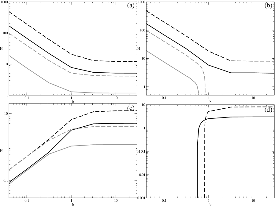
Figure 1: Distribution of the regions with different number of roots over the initial conditions space ($b\equiv b_{0}=b|_{t=0}$ and $H\equiv H_{0}=H|_{t=0}$) for the cases $\gamma_{\left(\mathbf{D}\right)}=+1,\,\{c_{0},c_{1},c_{2}\}=\{1,1,1\}$ in (a) panel, $\gamma_{\left(\mathbf{D}\right)}=+1,\,\{c_{0},c_{1},c_{2}\}=\{-1,1,1\}$ in (b) panel, $\gamma_{\left(\mathbf{D}\right)}=-1,\,\{c_{0},c_{1},c_{2}\}=\{1,1,1\}$ in (c) panel, and $\gamma_{\left(\mathbf{D}\right)}=-1,\,\{c_{0},c_{1},c_{2}\}=\{-1,1,1\}$ in (d) panel. Black line separate regions with four root (above the line) from region with two roots (below); grey line separate the region with two roots (above) from the region with no roots (below). Solid line corresponds to the $D=6$ case, while dashed – to the $D=16$ case (see text for details).

In Fig. 1 we plotted the distribution of the regions with different number of roots over the initial conditions space ($b\equiv b_{0}$ and $H\equiv H_{0}$). The roots in question are the roots of the eq. (11) – one can see that it is fourth order with respect to $\dot{b}_{0}$, so up to four real roots exists and the regimes and their distribution depends both on the number of roots and which branch (root) we choose. Here we explain and comment the roots distribution and below we give details on the regimes themselves. So in Fig. 1 we plotted these distribution: black line separate regions with four root (above the line) from region with two roots (below); grey line separate the region with two roots (above) from the region with no roots (below). Solid line corresponds to the $D=6$ case, while dashed – to the $D=16$ case – we plotted them both on the same graph to demonstrate the effect of the number of extra dimensions on the distribution.

Despite the fact that there is a continuous distribution of the three coupling constants ($c_{0}$, $c_{1}$, and $c_{2}$), all the cases for given $\gamma_{\left(\mathbf{D}\right)}$ could be brought to two – with positive and negative discriminant of (4) – the qualitative picture remains the same for the same $\gamma_{\left(\mathbf{D}\right)}$ and all combinations of ($c_{0}$, $c_{1}$, and $c_{2}$) which keep the same sign of the discriminant of (4). It makes the total number of cases four with both possible $\gamma_{\left(\mathbf{D}\right)}$. These four cases are presented in different panels of Fig. 1 – $\gamma_{\left(\mathbf{D}\right)}=+1,\,\{c_{0},c_{1},c_{2}\}=\{1,1,1\}$ (discriminant of (4) is negative) in (a) panel, $\gamma_{\left(\mathbf{D}\right)}=+1,\,\{c_{0},c_{1},c_{2}\}=\{-1,1,1\}$ (discriminant of (4) is positive) in (b) panel, $\gamma_{\left(\mathbf{D}\right)}=-1,\,\{c_{0},c_{1},c_{2}\}=\{1,1,1\}$ in (c) panel, and $\gamma_{\left(\mathbf{D}\right)}=-1,\,\{c_{0},c_{1},c_{2}\}=\{-1,1,1\}$ in (d) panel. One can see that panels (a) and (c) demonstrate all possible roots combinations – no roots (bottom region), two roots (middle one) and four roots (upper region), while panels (b) and (d) demonstrate quite different picture. The (c) case have no roots region, but it is compact, while (d) case does not have it at all.

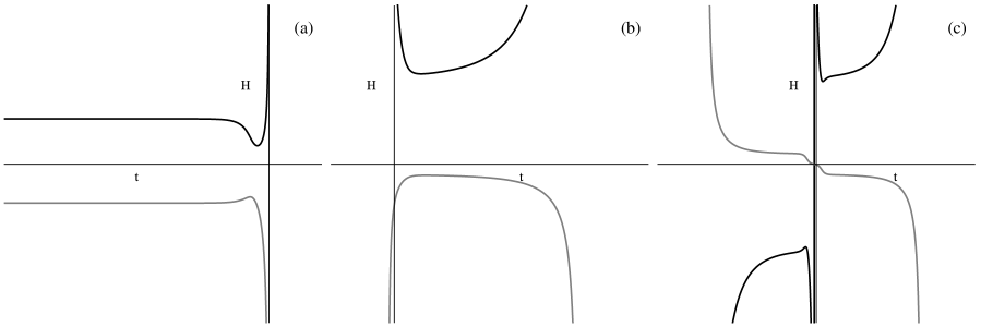
Figure 2: Regimes that are possible in $\gamma_{\left(\mathbf{D}\right)}=+1$ case with $\{c_{0},c_{1},c_{2}\}=\{1,1,1\}$ (see text for details).

After describing the distribution of the number of roots over the parameter space we are going to describe all possible regimes in the considered model. On the following figures black curves correspond to $H_{a}=H(t)$ variable while grey curves – to $H_{b}=\dot{b}(t)/b(t)$ – we decided that plotting the variables with the same dimensionality is better for demonstration.

In Fig. 2 we presented all regimes that are possible in $\gamma_{\left(\mathbf{D}\right)}=+1$ case with $\{c_{0},c_{1},c_{2}\}=\{1,1,1\}$. If there are two roots, both branches are like presented in Fig. 2(a); if there are four branches, one of them is like Fig. 2(a), two like Fig. 2(b), and the final is like Fig. 2(c). One can see that all three of them have finite time future singularity, which makes it impossible to describe our Universe. The only one of them which could compete for it, is Fig. 2(b) regime – with increase of $b_{0}$ (the “size” of curved extra dimension) its “lifetime” increases, so with large enough $b_{0}$ we can achieve long enough lifetime. But in turn it poses several problems, like how comes that initially the size of the extra dimension is that large, or it could even remains large enough to be detected nowadays.

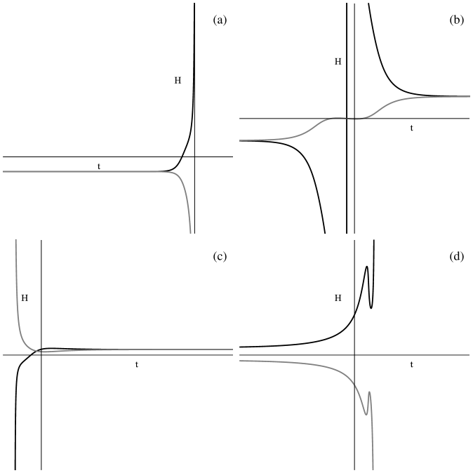
Figure 3: Additional regimes that are possible in $\gamma_{\left(\mathbf{D}\right)}=+1$ case (see text for details).

In Fig. 3 we presented all additional regimes that appear in $\gamma_{\left(\mathbf{D}\right)}=+1$ case. If there are two roots in $\gamma_{\left(\mathbf{D}\right)}=+1$ case with $\{c_{0},c_{1},c_{2}\}=\{-1,-1,1\}$, the regimes are like in Fig. 3(a) and Fig. 3(b); if there are four roots in that case, the regimes are: one like Fig. 3(a), two like Fig. 2(b), and the final one is like Fig. 3(b). Regime in Fig. 3(c) is replacing the Fig. 3(b) in the described above picture in the $\{c_{0},c_{1},c_{2}\}=\{-1,1,1\}$ case. All the remaining cases with different nonzero $c_{i}$ are one of the already described three cases according to the sign of the discriminant of the (4). Finally in Fig. 3(d) we presented a regime that appears in $c_{0}=0$ case, where it replaces Fig. 2(a) regime. The case with $c_{1}=0$ does not bring new regimes while $c_{2}=0$ reduces the system to the Friedman dynamics.

At this stage we want to stress the attention of the reader to several points. Comparing Figs. 3(a), (b), and (c) one cannot miss their familiarity. Indeed, Fig. 3(a) looks like left side of the Fig. 3(b), while Fig. 3(c) – like its right side. But there is a difference between Figs. 3(a) and (c) from one side and Fig. 3(b) from another – in the former case the singularity is standard, while in the latter it is what is called “nonstandard singularity”. This kind of singularity is “weak” by Tipler’s classification Tipler , and “type II” by Kitaura and Wheeler KW1 ; KW2 . Recent studies of the singularities of this kind in the cosmological context in Lovelock and Einstein-Gauss-Bonnet gravity demonstrates mpla09 ; grg10 ; gc10 ; prd10 that the presence of this singularity is not suppressed and it is abundant for a wide range of initial conditions. And in our case the singularities could “turn” one into another like in the just described above example. So one can see that in our case the presence of this nonstandard singularity is also not suppressed; one can see another example of it in Fig. 2(c); we discuss this type of singularity a bit additionally in Discussion.

Another point we want to stress an attention is the isotropisation and “antiisotropisation” issue. Comparing Fig. 2(a) with Fig. 3(a) one can see clearly that in former case we have $H_{b}=-H_{a}$ in the past asymptote while in the latter – it is $H_{b}=H_{a}$. The cause for that is the similar as in the classical cosmology – the presence of some isotropical matter, in our case it is an effective cosmological term (5). In Fig. 2(a) case we have $\{c_{0},c_{1},c_{2}\}=\{1,1,1\}$ so that $\Lambda_{eff}$ is imaginary and does not contribute to the dynamics – we have “antiisotropisation”. In contrast, in Fig. 3(a) we have $\{c_{0},c_{1},c_{2}\}=\{-1,1,1\}$ which gives us real $\Lambda_{eff}$ so that we have isotropisation. So that the $\Lambda_{eff}$ determines both the roots distribution and the regimes.

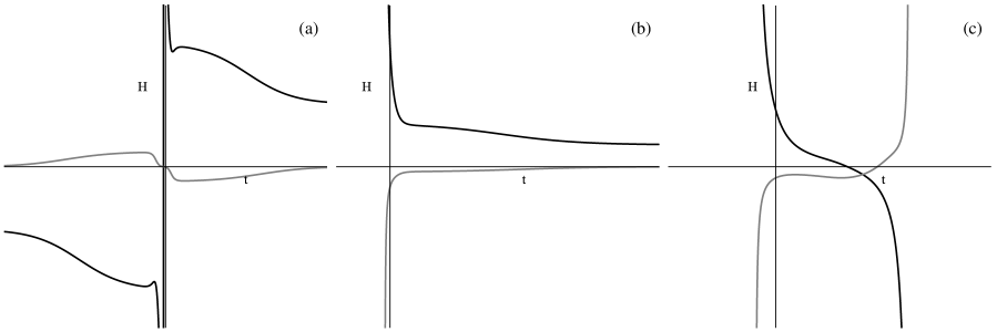
Figure 4: Additional regimes that appear in the $\gamma_{\left(\mathbf{D}\right)}=-1$ case (see text for details).

Overall, the cases with $\gamma_{\left(\mathbf{D}\right)}=+1$ do not give us “well-behaved” regimes because of the presence of finite time future singularities or because of isotropization, so we continue with $\gamma_{\left(\mathbf{D}\right)}=-1$ case. Generally, most of the regimes remains in $\gamma_{\left(\mathbf{D}\right)}=-1$ case, but some new regimes added; we present them in Fig. 4. From Fig. 4 one can immediately see that in (a) and (b) panels there are regimes without finite time future singularity and with “good” behavior – $H_{a}>0$ and $H_{b}<0$. The asymptotic behavior is like $H_{a}\to\mathop{\rm const}\nolimits$, $H_{b}\to 0$; the latter imply $b(t)\to b_{c}$. This is very attractive regime, and it occurs only in $\gamma_{\left(\mathbf{D}\right)}=-1$ case. The difference between Fig. 4(a) and Fig. 4(b) is clear – in the former case we have nonstandard singularity while in the latter we do not. The regime in the Fig. 4(c) could be considered as a counterpart for Fig. 2(c) but with no nonstandard singularity. The desired regime (in Fig. 4(b)) is one of the four roots in the $\gamma_{\left(\mathbf{D}\right)}=-1,\,\{c_{0},c_{1},c_{2}\}=\{1,1,1\}$ case and in the similar cases (that with imaginary $\Lambda_{eff}$ in the sense of (5)). Therefore all possible regimes the only physically reasonable one is when the theory does not admit a maximally symmetric vacuum and when the curvature of the extra dimensions is negative.

Up to here we considered only $\gamma_{(3)}=0$, but afterwards we confirmed the same results with both negative and positive $\gamma_{(3)}$, as the differences were only minor. More precisely, the $\gamma_{(3)}>0$ case has only Fig. 4(a) behavior while $\gamma_{(3)}<0$ has Fig. 4(b) as well. Also worth to mention, we have not detected numerically theoretically expected regime with both $a(t)\to\mathop{\rm const}\nolimits$ and $b(t)\to\mathop{\rm const}\nolimits$ – probably due to zero measure of the initial conditions which lead to it.

III Discussion and comments

In this paper we have investigated numerically the dynamical compactification for the most generic Einstein-Gauss-Bonnet gravity in arbitrary dimensions. Explicit time-dependence of the scale factors of both 3-space and extra dimensions is assumed. Moreover the constant curvatures of the space and compact dimensions were allowed to be independent and to have any sign. Perhaps the case of an extra dimensional manifold with negative constant curvature is less familiar. It is however important to stress that a manifold of negative constant curvature can be compactified by taking the quotient by a freely acting discrete subgroup so that it will have a finite volume MalMao . As the geometrically most simple compact manifold is a constant curvature one most simple there is no good a priori reason discarding a compact space with negative constant curvature. It is also important to stress that there is no problem to define gravity if the extra dimensions have negative constant curvature as the behavior of the graviton depends on the effective Newton constant defined from (6) as

$$\begin{array}[]{l}G_{N,eff}=(c_{1}(D+1)+2c_{2}(D-1)\Lambda_{D});\end{array}$$ (11)

from it one can see that the effective Newton constant depends only on coupling constant and not on curvature and through it negative constant curvature do not prevent effective (3+1)-dimensional gravity from being well-defined.

One of the important results of this paper is that the different dynamical regimes must be classified according to the value of the effective cosmological constant (5) rather then to the value of the “lambda term”.

It was found that most of the regimes do not lead to physically reasonable scenarios as they develop either finite future time singularities (standard or nonstandard) or isotropization of the entire space-time, where the size of the extra dimensions becomes of the same size than the one of the macroscopic three dimensional ones. It is worth pointing out that the singularities found in our analysis are quite different from the more common ones such as Big Rip and similar to them (see e.g. McInnes ; CKW ; ENOW ; NOT ) – indeed, in our case the singularities are anisotropic so that the volume of the entire space do not need to diverge – it could become singular or even remain constant – the latter is true for nonstandard singularities. With regard to the nonstandard singularities it is also worth mentioning that the same kind of singularity but called “determinant singularity” was found for Bianchi-I with dilaton in add14 . This proves that the nature of this “nonstandard singularity” lies entirely in nonlinearity of the equations of motion.

The only phenomenologically sensible scenario turned out to be the the case when the curvature of the extra dimensions is negative and when one chooses the region of the couplings space $\{c_{0},\,c_{1},\,c_{2}\}$ so that the theory does not admit a maximally symmetric vacuum solution (or in other words when the effective cosmological constant is complex). This scenario, which is independent from the sign of $\gamma_{(3)}$, can be interpreted as a symmetry breaking mechanism. Remarkably it does not require neither fine-tunings, as the region of the parameter space is an open set, nor violations of “naturalness hypothesis”. As we mentioned in the Introduction, the similar result – the dynamical compactification without violation of “naturalness” – was proposed in add13 for the (5+1)-dimensional EGB theory. As one can see, our setup is different from the one used in add13 – we considered both $M_{D}$ and $M_{4}$ as manifolds with constant and possibly nonzero curvature, which gives a rise to additional curvature terms and, as a consequence, to a new regime. Additionally, we considered all possible geometrical terms, including the volume term ($c_{0}\neq 0$), which crucially affects the dynamics. Overall, despite the fact that in both cases – in add13 and in our paper – we can see dynamical compactification, it is brought by different phenomena. In our case it is “geometric frustration” (see CGP1 ), which is brought by a combination of nonzero curvature and nonzero volume term – both of them are usually omitted from consideration since they complicate the equations a lot. The presence of non-zero curvature in the four dimensional part of the metric does not change qualitatively the the analysis.

In the analysis we have supposed the torsion to be zero. However in first order formalism the equations of motion of EGB gravity do not imply the vanishing of torsion which is therefore a propagating degree of freedom TZ-CQG . Indeed exact solutions with non-trivial torsion have been found CGT07 ; CGW07 ; CG ; CG2 ; ACGO . To study its effects in the context of dynamical compactification will be object of future investigation.

EGB gravity is the simplest generalization of General Relativity within the class of Lovelock gravity. As we considered an arbitrary number of extra dimensions it would also be interesting to study the effect of higher order Lovelock terms in the compactification mechanism. The results obtained in this paper suggest that the effects of higher terms depend sensibly on the fact if the highest curvature power is even as only in this case there exist a region in the parameter space which admits no maximally symmetric solution.

In the context of EGB theory existence of this region is solely due to the $c_{0}\neq 0$, as one can see from (5). Taking into consideration this ($c_{0}\neq 0$) case obviously makes the system far more difficult to solve – especially if one look for exact solutions – but it bears its fruits, as one can see. Indeed, when looking for exact solutions often only the simplest case is considered, and additional solutions are lost; this might be the case why this behavior has not been found earlier.

Acknowledgments.– This work was supported by FONDECYT grants 1120352, 1110167, and 3130599. The Centro de Estudios Cientificos (CECs) is funded by the Chilean Government through the Centers of Excellence Base Financing Program of Conicyt. We are also grateful for referees for their comments which help us improve the manuscript.

References

- (1) D. Lovelock, J. Math. Phys. 12, 498 (1971).
- (2) C. Garraffo and G. Giribet, Mod. Phys. Lett. A23, 1801 (2008).
- (3) T. Kaluza, Sit. Preuss. Akad. Wiss. K1, 966 (1921).
- (4) O. Klein, Z. Phys. 37, 895 (1926).
- (5) O. Klein, Nature 118, 516 (1926).
- (6) F. Canfora, A. Giacomini, R. Troncoso, and S. Willison, Phys. Rev. D80, 044029 (2009) [arXiv:0812.4311 [hep-th]].
- (7) F. Mller-Hoissen, Phys. Lett. 163B, 106 (1985).
- (8) J. Madore, Phys. Lett. 111A, 283 (1985).
- (9) J. Madore, Class. Quant. Grav. 3, 361 (1986).
- (10) F. Mller-Hoissen, Class. Quant. Grav. 3, 665 (1986).
- (11) H. Ishihara, Phys. Lett. B179, 217 (1986).
- (12) N. Deruelle, Nucl. Phys. B327, 253 (1989).
- (13) J. Kripfganz and H. Perlt, Acta Phys. Polon. B 18, 997 (1987).
- (14) T. Verwimp, Class. Quant. Grav. 6, 1655 (1989).
- (15) N. Deruelle and L. Faria-Busto, Phys. Rev. D 41, 3696 (1990).
- (16) J. Demaret, H. Caprasse, A. Moussiaux, P. Tombal, and D. Papadopoulos, Phys. Rev. D 41, 1163 (1990).
- (17) G. A. Mena Marugán, Phys. Rev. D 42, 2607 (1990).
- (18) G. A. Mena Marugán, Phys. Rev. D 46, 4340 (1992).
- (19) T. Torii and H. Maeda, Phys. Rev. D 71, 124002 (2005).
- (20) T. Torii and H. Maeda, Phys. Rev. D 72, 064007 (2005).
- (21) J. Grain, A. Barrau, and P. Kanti, Phys. Rev. D 72, 104016 (2005).
- (22) R. Cai and N. Ohta, Phys. Rev. D 74, 064001 (2006).
- (23) H. Maeda, Phys. Rev. D 73, 104004 (2006).
- (24) M. Nozawa and H. Maeda, Class. Quant. Grav. 23, 1779 (2006).
- (25) H. Maeda, Class. Quant. Grav. 23, 2155 (2006).
- (26) M. Dehghani and N. Farhangkhah, Phys. Rev. D 78, 064015 (2008).
- (27) E. Elizalde, A.N. Makarenko, V.V. Obukhov, K.E. Osetrin, and A.E. Filippov, Phys. Lett. B644, 1 (2007).
- (28) A. Toporensky and P. Tretyakov, Gravitation & Cosmology 13, 207 (2007).
- (29) S.A. Pavluchenko and A.V. Toporensky, Mod. Phys. Lett. A24, 513 (2009).
- (30) I.V. Kirnos, A.N. Makarenko, S.A. Pavluchenko, and A.V. Toporensky, Gen. Rel. Grav. 42, 2633 (2010).
- (31) I.V. Kirnos, S.A. Pavluchenko, and A.V. Toporensky, Gravitation & Cosmology 16, 274 (2010).
- (32) S.A. Pavluchenko, Phys. Rev. D 82, 104021 (2010).
- (33) F. Canfora, A. Giacomini and S. A. Pavluchenko, Phys. Rev. D 88, 064044 (2013)
- (34) K.I. Maeda and N. Ohta, Phys. Rev. D 71, 063520 (2005).
- (35) K.I. Maeda and N. Ohta, JHEP 1406, 095 (2014).
- (36) V.D. Ivashchuk, Int. J. Geom. Meth. Mod. Phys. 7, 797 (2010).
- (37) V.D. Ivashchuk, Gravitation & Cosmology 16, 118 (2010).
- (38) S.A. Pavluchenko, Phys. Rev. D 80, 107501 (2009).
- (39) S.A. Pavluchenko and A.V. Toporensky, Gravitation & Cosmology 20, 127 (2014).
- (40) D. Chirkov, S. Pavluchenko, and A.V. Toporensky, Mod. Phys. Lett. A29, 1450093 (2014).
- (41) D. Chirkov, S.A. Pavluchenko, and A.V. Toporensky, arXiv:1403:4625
- (42) S.A. Pavluchenko, Phys. Rev. D 67, 103518 (2003).
- (43) S.A. Pavluchenko, Phys. Rev. D 69, 021301 (2004).
- (44) J.A. Wolf, Spaces of constant curvature, 4th edition (Publish or Perish, Wilmington, Delaware USA, 1984), p. 69.
- (45) F.J. Tipler, Phys. Lett. A64, 8 (1977).
- (46) T. Kitaura and J.T. Wheeler, Nucl. Phys. B355, 250 (1991).
- (47) T. Kitaura and J.T. Wheeler, Phys. Rev. D 48, 667 (1993).
- (48) J. Maldacena and L. Maoz, JHEP 0402 053 (2004).
- (49) B. McInnes, JHEP 0208, 29 (2002).
- (50) R.R. Caldwell, M. Kamionkowski, and N.N. Weinberg, Phys. Rev. Lett. 91, 071301 (2003).
- (51) E. Elizalde, S. Nojiri, S.D. Odintsov, and P. Wang, Phys. Rev. D 71, 103504 (2005).
- (52) S. Nojiri, S.D. Odintsov, and S. Tsujikawa, Phys. Rev. D 71, 063004 (2005).
- (53) S. Alexeyev, A. Toporensky, and V. Ustiansky, Phys. Lett. B509, 151 (2001).
- (54) R. Troncoso and J. Zanelli, Class. Quant. Grav. 17, 4451 (2000) [arXiv:hep-th/9907109].
- (55) F. Canfora, A. Giacomini, and R. Troncoso, Phys. Rev. D 77, 024002 (2008).
- (56) F. Canfora, A. Giacomini, and S. Willison, Phys. Rev. D 76, 044021 (2007).
- (57) F. Canfora and A. Giacomini, Phys. Rev. D 78, 084034 (2008).
- (58) F. Canfora and A. Giacomini, Phys. Rev. D 82, 024022 (2010).
- (59) A. Anabalon, F. Canfora, A. Giacomini, J. Oliva, Phys. Rev. D 84, 084015 (2011).