Photometric, Astrometric and Polarimetric observations of gravitational microlensing events

Abstract

The gravitational microlensing as a unique astrophysical tool can be used for studying the atmosphere of stars thousands of parsec far from us. This capability results from the bending of light rays in the gravitational field of a lens which can magnify the light of a background source star during the lensing. Moreover, one of properties of this light bending is that the circular symmetry of the source is broken by producing distorted images at either side of the lens position. This property makes the possibility of the observation of the polarization and the light centroid shift of images. Assigning vectors for these two parameters, they are perpendicular to each other in the simple and binary microlensing events, except in the fold singularities. In this work, we investigate the advantages of polarimetric and astrometric observations during microlensing events for (i) studying the surface of the source star and spots on it and (ii) determining the trajectory of source stars with respect to the lens. Finally we analyze the largest sample of microlensing events from the OGLE catalog and show that for almost $\sim 4.3\%$ of events in the direction of the Galactic bulge, the polarization signals with large telescopes would be observable.

1 Introduction

The gravitational field of an astrophysical object can deviate the light path of a background source star and the result is the formation of two images at either side of the lens Einstein (1936). In the Galactic scale, the angular separation of the images is of the order of milli arc second, too small to be resolved by the ground-based telescopes. Instead, the overall light from the images received by the observer is magnified in comparison to an un-lensed source. This phenomenon is called gravitational microlensing and has been proposed as an astrophysical tool to probe dark objects in the Galactic disk. In recent years it has been used also for discovering the extra solar planets, the stellar atmosphere of distant stars and etc. Liebes (1964); Chang & Refsdal (1979); Paczyński 1986a,b . A detailed review on these topics can be found in Gaudi (2012). An important problem in photometric observations of microlensing events is the degeneracy between the lens parameters as the distance, mass and velocity. We can partially resolve this degeneracy by using higher order terms as the parallax and finite size effects which can slightly change simple microlensing light curves. However, these effects can not be applied for all the microlensing events. There are other observables such as (i) the centroid shift of images and (ii) the polarization variation of images during the lensing that can break this degeneracy. Here, we assume that during photometric observations of microlensing events, polarimetric and astrometric observations also can be done.

Astrometric observation: In the gravitational microlensing, the light centroid of images deviates from the position of the source star and for the case of a point-mass lens, the centroid of images traces an elliptical shape during the lensing Walker (1995); Miyamoto & Yoshii (1995); Høg et al. (1995); Jeong et al. (1999). By measuring the light centroid shift of images with the high resolution ground-based or space-based telescopes, accompanied by measurements of the parallax effect, the lens mass can be identified Paczyński (1997); Miralda-Escdé (1996). This method is also applicable for studying the structure of the Milky way with enough number of microlensing events Rahvar & Ghassemi (2005). Also the degeneracy in the close and the wide caustic-crossing binary microlensing events can be removed by astrometric observations Dominik (1999); Gould & Han (2000); Chung et al. (2009).

Polarimetric observation: Another feature in the gravitational microlensing is the time-dependent variation of the polarization during the lensing. The scattering of photons by electrons in the atmosphere of star makes a local polarization in different positions over the surface of a star and as a result of circular symmetry of the star, the total polarization is zero Chandrasekhar (1960); Sobolev (1975). During the gravitational microlensing, the circular symmetry of images breaks and the total polarization of source star is non-zero and changes with time Schneider & Wagoner (1987); Simmons et al. 1995a,b ; Bogdanov et al. (1996). Measuring polarization during microlensing events helps us to evaluate the finite source effect, the Einstein radius and the limb-darkening parameters of the source star Yoshida (2006); Agol (1996); Schneider & Wagoner (1987).

In this work we start with the investigation for a possible relation between the polarization and the centroid shift vectors. We find an orthogonality relation between them in the simple as well as the binary lensing. However, near the cusp in the caustic lines of a binary lens, the polarization and centroid shift vectors are not normal to each other except on the symmetric axis of the cusp. This effect enables us to discover the source trajectory relative to the caustic line. As a result of this orthogonality relation, the polarimetry measurements can resolve the source trajectory degeneracy, i.e. $u_{0}$ degeneracy, in the same way as the astrometric observations. Finally, we study the effects of source spots as a perturbation effect and show that they can break this orthogonality relation. Studying the time variation of polarization can provide a unique tool to distinguish and study the source anomalies such as spots on the surface of the source stars.

The layout of the paper is as follows. In sections (2) we introduce the polarization and astrometry in the gravitational lensing and demonstrate that there is an orthogonality relation between them in simple microlensing events. We extend this discussion for the binary lensing in section (3) and discuss how this correlation helps to resolve the degeneracy problem. In section (4), we investigate the effect of source spots in the polarimetric observation. Finally, we take the largest sample of the OGLE microlensing data and estimate the number of events with the observable polarimetry signals. We conclude in section (5).

2 Polarimetric and Astrometric shift in gravitational microlensing

In this section we first review the polarization during microlensing events. Then we study the astrometric shift and its orthogonality with the polarization for an extended source star.

2.1 Polarization during gravitational microlensing

Chandrasekhar (1960) has shown that photons can be scattered by electrons (Thompson scattering) in the atmosphere of hot stars which makes a linear and local polarization. The amount of polarization enhances from the centre to the limb and at a given wavelength in each point it is proportional to the cosine of the angle between the line of sight and the normal vector to the star surface. The other mechanisms such as photon scattering on atomic, molecular species and neutral hydrogen (Rayleigh scattering) or on dust grains are also responsible for producing a local polarization over late-type main sequence and cool giant stars Ingrosso et al. (2012). Due to the circular symmetry of the star surface, the total light of a distant star is unpolarized. This circular symmetry can be broken by spots on the star surface, magnetic fields or the lensing effect and as a result, we expect to detect a non-zero polarization for these cases. For example, the emission lines from T-Tauri stars (pre-main sequence stars) show a linear polarization due to the light scattering by dust grains in the circumstellar disk around the central stars. This polarization changes with time due to variations in the configuration of the dust pattern Drissen et al. (1989); Akitaya et al. (2009).

Schneider & Wagoner (1987) noticed that there is a net and time-dependent polarization for a lensed supernova. They estimated the amounts of polarization degree near point and critical line singularities. The existence of a net polarization during microlensing events due to circular symmetry breaking was noticed by Simmons et al. (1995a,b) and Bogdanov et al. (1996). Also, polarization in binary microlensing events was numerically calculated by Agol (1996). He noticed that in a binary microlensing event, the net polarization is larger than that by a single lens and reaches to one percent during the caustic crossing. A semi-analytical formula for polarization degree induced by a single microlens was derived by Yoshida (2006). Recently, Ingrosso et al. (2012) evaluated the expected polarization signals for a set of reported high-magnification single-lens and exo-planetary microlensing events towards the Galactic bulge. They showed that it reaches to $0.04$ per cent for late-type stars and rises to a few per cent for cool giants.

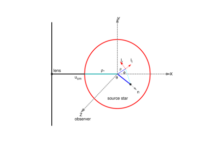
Figure 1: Demonstration of a projected source surface on the lens plane (red circle). In this figure, the black star and the black spot represent the lens position and a typical point on the source surface, respectively. Source star is projected on the sky plane. The directions of $\bm{n}$ and $\bm{Z}$ refer to the propagation direction and line of sight towards the observer. $u_{cm}$ connects lens position to the source center, $\phi$ is the azimuthal angle between the lens-source connection line and the line from the origin to each projected element over the source surface and $\theta$ is the projection angle i.e. $\rho=\sin\theta$. $\bm{l_{l}}$ and $\bm{l_{r}}$ are two unit vectors normal to the direction of $\bm{Z}$ as shown in the figure.

In this part, we review how to calculate the net polarization of a source star in the microlensing events. For describing the polarized light, we use $S_{I}$, $S_{Q}$, $S_{U}$ and $S_{V}$ as the Stokes parameters. These parameters show the total intensity, two components of linear polarizations and the circular polarization over the source surface, respectively Tinbergen (1996). For a stellar atmosphere, we set the circular polarization to be zero, $S_{V}=0$. The linear polarization degree $(P)$ and angle of polarization $(\theta_{p})$ as functions of total Stokes parameters are given by Chandrasekhar (1960):

$$P = \frac{\sqrt{S_{Q}^{2}+S_{U}^{2}}}{S_{I}},$$

$$\theta_{p} = \frac{1}{2}\tan^{-1}{\frac{S_{U}}{S_{Q}}},$$ (1)

where the un-normalized Stokes parameters are defined as follows:

$$S_{Q} \equiv \int_{\mathcal{S}}d^{2}\mathcal{S}<E_{X}E_{X}-E_{Y}E_{Y}>=$$

$$= -\int d^{2}\mathcal{S}~{}I_{-}(\mu)\cos(2\phi),$$

$$S_{U} \equiv -\int_{\mathcal{S}}d^{2}\mathcal{S}<E_{X}E_{Y}+E_{Y}E_{X}>=$$

$$= \int d^{2}\mathcal{S}~{}I_{-}(\mu)\sin(2\phi),$$

$$S_{I} \equiv \int_{\mathcal{S}}d^{2}\mathcal{S}<E_{X}E_{X}+E_{Y}E_{Y}>=\int d^{2}\mathcal{S}~{}I(\mu),$$ (2)

where $\mathcal{S}$ refers to source area projected on the lens plane, $\phi$ is the azimuthal angle between the lens-source connection line and the line from the origin to each element over the source surface, $I(\mu)=I_{l}(\mu)+I_{r}(\mu)$, $I_{-}(\mu)=I_{r}(\mu)-I_{l}(\mu)$ and $<>$ refers to the time averaging (see Figure 1). In following, we adapt the coordinate sets used by Chandrasekhar. Let us define $\bm{n}$ being the normal to the source surface at each point which is the propagation direction and $\bm{Z}$ being the direction towards the observer. We define $\bm{r}$ and $\bm{l}$ so that $I_{l}(\mu)$ being the emitted intensity by the star atmosphere in the plane containing the line of sight and the normal to the source surface on that point, i.e. $(\bm{n})$, and $I_{r}(\mu)$ being the emitted intensity in the normal direction to that plane, where $\bm{r}\times\bm{l}=\bm{Z}$, $\mu=\cos(\theta)=\sqrt{1-\rho^{2}}$ and $\rho$ is the distance from the centre to each projected element over the source surface normalized to the projected radius of star on the lens plane. Indeed, $\bm{l}$ represents the radial and $\bm{r}$ is the tangent coordinates perpendicular to the line of sight. We consider a fixed cartesian coordinate at the star centre where $\bm{X}$-axis is outwards the lens position, $\bm{Y}$-axis is normal to it, projected in the sky plane and $\bm{Z}$-axis is in the line of sight towards the observer. The projected source surface on the lens plane (red circle) and the specified axes are shown in Figure (1).

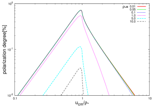
Figure 2: The polarization degree versus $u_{cm}/\rho_{\star}$ for different values of star size and impact parameter. The polarization raises to a maximum value at $u_{cm}/\rho_{\star}\approx 0.96$ ( Schneider & Wagoner 1987).

In simple microlensing events, the Stokes parameters by integrating over the source surface are given by:

$$\left(\begin{array}[]{c}S_{Q}\\ S_{U}\end{array}\right) = \rho^{2}_{\star}\int_{0}^{1}\rho~{}d\rho\int_{-\pi}^{\pi}d\phi I_{-}(\mu)A(u)\left(\begin{array}[]{c}-\cos 2\phi\\ \sin 2\phi\end{array}\right),$$ (7)

$$S_{I} = ~{}\rho^{2}_{\star}\int_{0}^{1}\rho d\rho\int_{-\pi}^{\pi}d\phi I(\mu)~{}A(u),$$ (8)

where $\rho_{\star}$ is the projected radius of star on the lens plane and normalized to the Einstein radius, $u=(u_{cm}^{2}+\rho^{2}\rho^{2}_{\star}+2\rho\rho_{\star}u_{cm}\cos\phi)^{1/2}$ is the distance of each projected element over the source surface with respect to the lens position, $u_{cm}$ is the impact parameter of the source centre and magnification factor for a simple microlensing is

$$A(u)=\frac{u^{2}+2}{u\sqrt{u^{2}+4}}.$$

The amounts of $I(\mu)$ and $I_{-}(\mu)$ by assuming the electron scattering in spherically isotropic atmosphere of an early-type star were evaluated by Chandrasekhar (1960) as follows

$$I(\mu) = I_{0}(1-c_{1}(1-\mu)),$$

$$I_{-}(\mu) = I_{0}c_{2}(1-\mu),$$ (9)

where $c_{1}=0.64$, $c_{2}=0.032$ and $I_{0}$ is the total intensity emitted towards the line of sight direction Schneider & Wagoner (1987).

For a point-mass lens, the integrals over the azimuthal angle $\phi$ of the total Stokes parameters, i.e. equation (7), are reduced to a combination of complete elliptical integrals Yoshida (2006). We calculate the Stokes parameters by numerical integrations. Figure (2) represents the dependence of the polarization degree on the source size, $\rho_{\star}$ and $u_{cm}/\rho_{\star}$. The polarization has its maximum value at $u_{cm}/\rho_{\star}\approx 0.96$ Schneider & Wagoner (1987). If $u_{0}<\rho_{\star}$ there are two times in which $u_{cm}=0.96\rho_{\star}$, so the time profile of polarization has two peaks (transit case) whereas if $u_{0}\geq\rho_{\star}$ only in the closest approach the time profile of the polarization has a peak (bypass case) Simmons et al. 1995b . For the case that the finite size effect of source star is small, the probability of detecting polarization also is small as the chance that the lens and source approach with the impact parameter comparable to the source size is small. Hence, detecting polarization effect is in favour of microlensing events with a large finite size parameter (i.e. giant stars).

According to equation (7), the total Stokes parameter $S_{U}$ for a limb-darkened and circular source in simple Paczyński microlensing events is zero and $S_{Q}$ is negative. Hence, the net polarization is normal to the lens-source connection line. In figure (3), we show the polarization map around a point-mass lens located at the centre of the plane with solid black lines. Note that, the size of lines is proportional to the polarization. The orientation (i.e. $\theta_{p}$) is given in terms of its angle with respect to the x-axis specified in Figure (1). The arrow sign represents the centroid shift of images that will be discussed in the next part.

2.2 Astrometric centroid shift

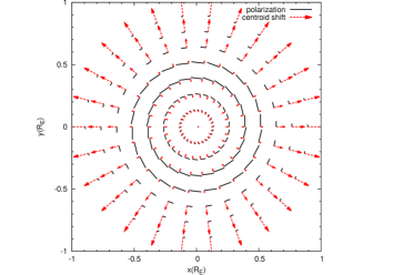
Figure 3: The astrometric (red dashed vectors) and polarimetric maps (black solid lines) around a point-mass lens located at centre of plane. We set $\rho_{\star}=0.5$. Note that, the size of centroid shifts and polarizations are normalized by the arbitrary factors. For $u\simeq\rho_{\star}$, the size of the centroid shift vector tend to zero while polarization signal is maximum.

In gravitational microlensing events a shift in the light centroid of the source star happens with respect to its real position. For a point-mass lens the astrometric shift in the light centroid is defined by:

$$\bm{\delta\theta}_{c}=\frac{\mu_{1}\bm{\theta_{1}}+\mu_{2}\bm{\theta_{2}}}{\mu_{1}+\mu_{2}}-\bm{u}\theta_{E}=\frac{\theta_{E}}{u^{2}+2}\bm{u},$$ (10)

where $\theta_{E}$ is the angular size of the Einstein ring. The astrometric shift traces an ellipse, so-called the astrometric ellipse while the source star passes an straight line with respect to the lens plane Walker (1995); Jeong et al. (1999). The ratio of axes for this ellipse is a function of the impact parameter and for large impact parameters this ellipse converts to a circle whose radius decreases by increasing the impact parameter and for small values, it turns to a straight line Walker (1995). In Figure (3), we plot a vector map containing the normalized astrometric centroid shift at each position of the lens plane which is a symmetric map around the position of a point-mass lens. All the vectors in this case are radial and outward.

The astrometric centroid of an extended source is given by (Witt & Moa 1998)

$$\bm{\theta}^{fs}_{c}=\frac{1}{\pi\rho^{2}_{\star}\bar{I}\mu^{fs}}\sum_{i}\int_{\mathcal{S}}d^{2}\mathcal{S}~{}I(\bm{u})\bm{\theta}_{i}\mu_{i},$$ (11)

where $\bar{I}$ is the mean surface brightness of source, $\bm{\theta}_{i}$ is the position of the $i$th image with the magnification factor $\mu_{i}$ and $\mu^{fs}$ is the total magnification factor of an extended source:

$$\mu^{fs}=\frac{1}{\pi\rho^{2}_{\star}\bar{I}}\sum_{i}\int_{\mathcal{S}}d^{2}\mathcal{S}~{}I(\bm{u})\mu_{i}(\bm{u}).$$ (12)

In a simple microlensing event, where we have a single lens and the surface brightness of source star is uniform, $\sum_{i}\bm{\theta}_{i}\mu_{i}=\theta_{E}\frac{u^{2}+3}{\sqrt{u^{2}+4}}\hat{u}$ and the normalized centroid shift for an extended source is given by:

$$\bm{\delta\theta}_{c}^{fs}(\theta_{E})=-\bm{u_{cm}}+\frac{1}{\pi\mu^{fs}}\int_{0}^{1}\rho d\rho\int_{-\pi}^{\pi}d\phi I(\rho)\frac{u^{2}+3}{\sqrt{u^{2}+4}}\hat{u},$$ (13)

where $\hat{u}=(\rho\cos\phi+u_{cm},\rho\sin\phi)/u$ (see Figure 1). In Figure (4), we plot the trajectories of normalized centroid shifts in the lens plane (upper panel) and the absolute value of normalized centroid shifts versus $u$ (lower panel) for different values of $\rho_{\star}$ and fixed value of $u_{0}=0.1$.

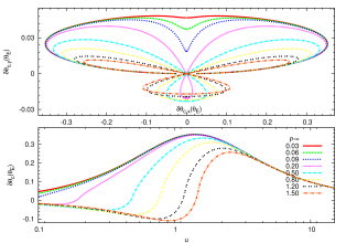
Figure 4: The normalized centroid shift trajectories in the lens plane (upper panel) and the normalized centroid shift amount versus $u$ (lower panel) for different amounts of $\rho_{\star}$ and $u_{0}=0.1$. The negative value of centroid shift (in lower panel) indicates reverting its direction with respect to the $x$-axis which occurs for $u\leq\rho_{\star}$.

In the case of a uniform or limb-darkened source, the centroid shift component normal to the lens-source connection line (i.e. $Y$-axis in Figure 1) is zero. On the other hand, the polarization orientation is normal to the centroid shift for a single lens (see Figure 3). The anomalies over the source surface can break this orthogonal relation. We note that, astrometric signals are detectable for the nearby and massive lenses which have large angular Einstein radii. On the other hand polarimetric signals are sensitive to high-magnification microlensing events or extended sources where we have the condition of $u_{cm}\simeq\rho_{\star}$.

3 Binary microlenses

In this section we investigate a possible relation between the polarization and the astrometric centroid shift in binary microlensing events. In these events, the polarization signal when the source star crosses the caustic curve is higher than that in the single lens case Agol (1996). The caustic lines can be classified into two categories of (i) folds where the caustic lines are smooth and (ii) cusps where folds cross at a point Petters & Witt (1996). We will investigate the polarization and astrometric signals near fold and cusp singularities.

Assuming that a source star crosses the fold of a caustic curve, two temporary images can appear on the lens plane with almost the same magnification factors Schneider et al. 1992a . On the other hand, there are global images which do not change during caustic crossing. These global images move slowly and have small magnification factors with respect to the temporary images. Hence, we only consider the temporary images and obtain their light centroid and polarization vectors in our calculation. We set the centre of coordinate located at the fold and axes are parallel with and normal to the tangent vector of the fold. We also connect the source centre to the centre of coordinate i.e. $\bm{u}_{cm}=(0,z\rho_{\star})$, therefore, the position of any point on the source surface in this coordinate is given by $\bm{u}=\bm{u}_{cm}+\rho_{\star}\bm{\rho}$. Since the position vector of local images due to the fold singularity, $\bm{\theta}_{\pm}$ is a linear function with respect to $\bm{u}$, hence $\bm{\theta}_{\pm}(\bm{u})=\bm{\theta}_{\pm}(\bm{u}_{cm})+\rho_{\star}\bm{\theta}_{\pm}(\bm{\rho})$. The magnification factor for these images is

$$\mu_{\pm}=\frac{1}{2}\sqrt{\frac{u_{f}}{\rho_{\star}(\rho_{2}+z)}}$$

where $\rho_{2}\geq-z$. The light centroid of images near the fold singularity is given by Gaudi & Petters (2002):

$$\bm{\theta}^{fs}_{f} = \bm{\theta}_{f,cm}+\frac{\sqrt{u_{f}\rho_{\star}}}{\pi\mu^{fs}_{f}ad}\int_{max(-z,-1)}^{1}d\rho_{2}\int_{-\sqrt{1-\rho^{2}_{2}}}^{\sqrt{1-\rho^{2}_{2}}}$$ (16)

$$d\rho_{1}I(\rho)\frac{1}{\sqrt{\rho_{2}+z}}\left(\begin{array}[]{c}d\rho_{1}-b\rho_{2}\\ -b\rho_{1}\end{array}\right),$$

where $\rho=\sqrt{\rho^{2}_{1}+\rho^{2}_{2}}$ and $\bm{\theta}_{f,cm}=(\frac{-b\rho_{\star}}{ad}z,0)$ which is parallel with the $u_{1}$-axis. For a limb-darkened source star, $y$ component of the second sentence vanishes due to the symmetric range of $\rho_{1}$. Hence, near the fold singularities the centroid shift vector is parallel with the caustic (i.e. $u_{1}$).

On the other hand the Stokes parameters near the fold are given by:

$$\left(\begin{array}[]{c}S_{Q}\\ S_{U}\end{array}\right) = \sqrt{\frac{u_{f}}{\rho_{\star}}}\int_{max(-z,-1)}^{1}d\rho_{2}\int_{-\sqrt{1-\rho^{2}_{2}}}^{\sqrt{1-\rho^{2}_{2}}}$$ (22)

$$d\rho_{1}I_{-}(\rho)\frac{1}{\rho^{2}\sqrt{\rho_{2}+z}}\left(\begin{array}[]{c}\rho^{2}_{1}-\rho^{2}_{2}\\ 2\rho_{1}\rho_{2}\end{array}\right).$$

Here, the second component (i.e. $S_{U}$) due to the symmetry of integral over $\rho_{1}$ is zero. As a result, near the fold singularities polarizations are normal to the tangent vector to the fold and the centroid shift vectors. According to this orthogonality relation near the fold singularity, the polarimetry and astrometry can provide the following information of (i) tracing the source trajectory with respect to caustic lines, (ii) in the case that the orthogonality relationship is broken, we can study possible effects of anomalies such as spots over the source surface. The orthonormality relation can also be broken in cusp singularities except for the case that the source is located at symmetric axis of the cusp. For other points around the cusp, this orthogonal relation does not exit. We calculate numerically the polarization and centroid shift vectors around the cusp shown in Figure (5).

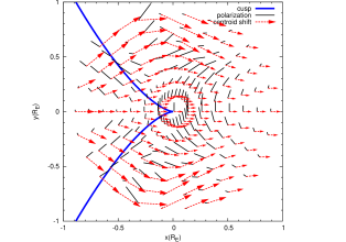
Figure 5: The polarization (black lines) and astrometric centroid shift (red vectors) near the cusp in a binary lens (blue line). We set $\rho_{\star}=0.5$. Note that, the size of centroid shifts and polarizations are divided by constant factors. Whenever the limb of the source star crosses the cusp, the polarization signal strongly changes.

4 The effect of source spots on polarization and centroid shift

In this section we study the effect of source spots on polarization and centroid shift of microlensing events. Our aim is to extract the astrophysical information of the spots and the atmosphere of the source star from these anomalies.

A given spot on the source star with a different temperature and magnetic field in comparison to the background star produces an angular-dependent defect on the source surface. The result is producing a net polarization even in the absence of the gravitational lensing. The gravitational lensing can amplify the polarization as well as change the orientation of the polarization. The amount of magnified polarization depends on relative position of spots with respect to the source centre and the lens position. Also it depends on the temperature and intrinsic flux of spots.

Here we use three parameters to quantify a spot in our calculation as: (i) the size of the spot, (ii) the temperature of the source star and its temperature difference with respect to the spot and (iii) the location of the spot on the source surface. Let us characterize the lens plane by $(u_{1},u_{2})$ axes and put the centre of lens at the centre of coordinate system. The projected positions of the source and the spot in this reference frame are $(u_{1,\star},u_{2,\star})$ and $(u_{1,s},u_{2,s})$. The radius of the spot is $r_{s}$ and its angular size in the coordinate system located at the centre of source star is given by $\theta_{0}=\sin^{-1}(r_{s}/R_{\star})$. For simplicity we choose a circular spot over the source surface. In order to locate a typical spot on the source star, we first put the position of the spot at the star pole and then perform a coordinate transformation and move the spot to an arbitrary location of the source Mehrabi & Rahvar (2014). The position of the spot located at the pole of the spherical coordinate system is given by:

$$X_{s} = R_{\star}\sin\eta\cos\varphi$$

$$Y_{s} = R_{\star}\sin\eta\sin\varphi$$

$$Z_{s} = R_{\star}\cos\eta,$$ (23)

where $\eta$ and $\varphi$ change in the ranges of $[0,\theta_{0}]$ and $[0,2\pi]$, respectively. The spot position projected on the lens plane and normalized to the Einstein radius is

$$x_{s} = \rho_{\star}\sin\eta\cos\varphi$$

$$y_{s} = \rho_{\star}\sin\eta\sin\varphi$$

$$z_{s} = \rho_{\star}\cos\eta,$$ (24)

and finally the spot position on the lens plane, using two rotation angles of $\theta$ around $y$-axis and $\phi$ around $z$-axis is given by

$$u_{1,s} = x_{s}\cos\phi\cos\theta-y_{s}\sin\phi+z_{s}\cos\phi\sin\theta+u_{1,\star}$$

$$u_{2,s} = x_{s}\sin\phi\cos\theta+y_{s}\cos\phi+z_{s}\sin\phi\sin\theta+u_{2,\star}.$$ (25)

The modified Stokes parameters $S^{\prime}_{Q}$, $S^{\prime}_{U}$ and $S^{\prime}_{I}$ for the case of a single spot on the source are given by:

$$\left(\begin{array}[]{c}S^{\prime}_{Q}\\ S^{\prime}_{U}\end{array}\right) = \left(\begin{array}[]{c}S_{Q}\\ S_{U}\end{array}\right)-f\int_{\mathcal{A}_{s}}d^{2}s~{}I_{-}(\rho)A(u_{s})\left(\begin{array}[]{c}-\cos 2\phi\\ \sin 2\phi\end{array}\right)$$ (32)

$$= \left(\begin{array}[]{c}S_{Q}\\ S_{U}\end{array}\right)-f\left(\begin{array}[]{c}S_{Q,s}\\ S_{U,s}\end{array}\right),$$ (37)

$$S^{\prime}_{I} = S_{I}-f\int_{\mathcal{A}_{s}}d^{2}s~{}I(\rho)A(u_{s})=S_{I}-fS_{I,s},$$ (38)

where $S_{Q}$, $S_{U}$ and $S_{I}$ are given by the equation (7), these parameters assigned for the source star without any spot and ${\mathcal{A}_{s}}$ represents area that is covered by the spot. $u_{s}=\sqrt{u_{1,s}^{2}+u_{2,s}^{2}}$ is the distance of each point of the spot from the lens position and $f=\left[F_{\star}(\nu)-F_{\mathcal{A}_{s}}(\nu)\right]/F_{\star}(\nu)$ is the relative difference in the flux of the source and spot at the frequency of $\nu$. We assume a black-body radiation for both star and spot. The polarization degree $P^{\prime}$ also can be given by:

$$P^{\prime}=\frac{\left(P^{2}S_{I}^{2}+f^{2}P_{s}^{2}S_{I,s}^{2}-2fC(P,P_{s})S_{I}S_{I,s}\right)^{1/2}}{S_{I}-fS_{I,s}},$$ (39)

where we define $P_{s}\equiv({S_{Q,s}^{2}+S_{U,s}^{2}})^{1/2}/S_{I,s}$ and $C(P,S_{s})\equiv(S_{Q}S_{Q,s}+S_{U}S_{U,s})/S_{I}S_{I,s}$ as the cross term between the contribution from the star and spot. The angle of polarization $\theta^{\prime}_{p}$ in terms of the Stocks parameters of the source and spot is given by

$$\theta^{\prime}_{p} = \frac{1}{2}\tan^{-1}[\frac{S_{U}}{S_{Q}}+f\frac{S_{U}S_{Q,s}-S_{Q}S_{U,s}}{S^{2}_{Q}}$$ (40)

$$+ f^{2}\frac{-S_{Q,s}S_{U,s}S_{Q}+S_{U}S^{2}_{Q,s}}{S^{3}_{Q}}+...].$$

We can rewrite this equation in terms of unperturbed angle $\theta_{p}$ and first- and second-order terms in $f$ as follows:

$$\theta^{\prime}_{p} = \theta_{p}+f\frac{S_{U}S_{Q,s}-S_{Q}S_{U,s}}{2P^{2}S^{2}_{I}}$$ (41)

$$+ f^{2}\frac{C(P,P_{s})S_{I,s}}{2P^{4}S^{3}_{I}}(S_{U}S_{Q,s}-S_{Q}S_{U,s})+...$$

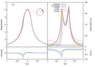
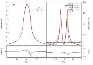
Figure 6: The two microlensing events with spot on sources. In both subfigures (a) and (b), the light curves and polarimetric curves with different set of parameters for the spot are shown in left and right panels, respectively. The source (grey circle) and its spot (pink spot), lens position (grey star) and source centre trajectory projected in the lens plane (red dash-dotted line) are shown with insets in the left-hand panels. The simple models without spot effect are shown by red solid lines. The black horizontal dashed lines represent the polarization signals due to spotted sources without lensing effect. The photometric and polarimetric residuals with respect to the simple models are plotted in bottom panels. The parameters of these microlensing events shown in subfigure $(a)$ and $(b)$ are $\rho_{\star}=0.3$, $\theta=80^{\circ}$, $\phi=30^{\circ}$, $u_{0}=-0.205$, $f=0.9$ and $\rho_{\star}=0.21$, $\theta=110^{\circ}$, $\phi=10^{\circ}$, $u_{0}=-0.033$, $r_{s}=0.35\rho_{\star}$, respectively.

In Figures (6) we represent two microlensing events considering a stellar spot on the source surface. In both cases, we plot the photometric and polarimetric light curves. The parameters of these microlensing events shown in subfigures $(a)$ and $(b)$ are $(a)$ $\rho_{\star}=0.3$, $\theta=80^{\circ}$, $\phi=30^{\circ}$, $u_{0}=-0.205$, $f=0.9$ and $(b)$ $\rho_{\star}=0.21$, $\theta=110^{\circ}$, $\phi=10^{\circ}$, $u_{0}=-0.033$, $r_{s}=0.35\rho_{\star}$, respectively. Interpreting Figure (6), the polarimetric curve in the absence of stellar spots for the case of $u_{0}<\rho_{\star}$ has two symmetric peaks at $t(t_{E})=t_{0}\pm\sqrt{\rho_{\star}^{2}-u_{0}^{2}}$ where $t_{0}$ is the time of the closest approach. For the case of a spot on the source surface, not only the symmetry in the pholarimetic curve breaks, also it tends to non-zero polarization at no-lensing stages.

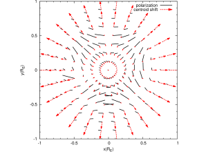
Figure 7: The normalized polarization (black lines) and astrometric centroid shift (red vectors) for a source star with stellar spot lensed by a point-mass lens with the parameters of $\rho_{\star}=0.5$, $\theta_{0}=18^{\circ}$, $\theta=110^{\circ}$, $\phi=15^{\circ}$ and $f=0.75$. Note that, the size of centroid shifts and polarizations are normalized by an arbitrary factor.

A significant signal of the stellar spot in microlensing events happens when the lens approaches close enough to the spot. In that case the total flux due to the spot $S_{I,s}$ increases and as a result denominator of equation (39) decreases. On the other hand, the cross term $C(P,P_{s})$ enhances, as $P$ is approximately parallel with $P_{s}$ (noting that, the polarimetric vectors over the spot are similar to the polarimetric vectors over the source except having different temperatures). Moreover, if the spot is located on the limb of the source star, one of peaks in the polarimetric curve will strongly be disturbed. According to Figure (6), the larger and darker spots make stronger polarimetric and photometric signals. We note that the presence of the spot has small effects on light curves.

The astrometric centroid shift of a source with a spot is given by:

$$\bm{\delta\theta}^{\prime}_{c}=\frac{1}{S^{\prime}_{I}}\{S_{I}\bm{\theta}_{c}-f\int_{\mathcal{A}}d^{2}s~{}I(\rho)\frac{u_{s}^{2}+3}{u_{s}\sqrt{u_{s}^{2}+4}}$$

$$\left(\begin{array}[]{c}\rho\cos\phi+u_{cm}\\ \rho\sin\phi\end{array}\right)\}-\bm{u}_{spot},$$ (44)

where $\bm{\theta}_{c}$ is the light centroid vector for a source star without any spot (see equation 13) and $\bm{u}_{spot}$ is the light centroid of the source with a spot. The spot perturbation on the astrometric measurements is larger for the smaller impact parameters. In Figure (7), we plot the map of normalized polarization and centroid shift vectors of the source with a spot and the parameters of $\rho_{\star}=0.5$, $r_{s}=0.3\rho_{\star}$, $\theta=110^{\circ}$, $\phi=15^{\circ}$, and $f=0.75$, lensed by a single lens. We note that the orientations of polarization and centroid shift in the absence of the spot are orthogonal. The polarization vector changes strongly due to the spot while the centroid shift is almost unchanged except for the close approaches. As a result, the anomalies over the source surface break the orthogonality relation between the astrometric centroid shift and polarization vectors.

4.1 Statistical investigation of the OGLE data for polarimetry observation

Here we investigate the statistics of high magnification events in the list of the OGLE data to identify the fraction of events with possible signatures of the polarization. For the case of high magnification events with $u_{0}<\rho_{\star}$, the time profile of polarization has two peaks and the maximum polarization may reach to one percent. The large telescopes with enough exposure times can achieve the sensitivity of detecting the polarization as well as time variation of this parameter. In a recent work by Ingrosso et al. (2012), they prospect the observation of the polarization by FOcal Reducer and low dispersion Spectrograph 2 (FORS2) on the Very Large Telescope (VLT). A detailed study for follow-up observations of polarization of the OGLE microlensing data will be presented in a later work.

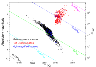
Figure 8: Temperature-Luminosity diagram for the OGLE microlensing events with main-sequence (black points) and red clump sources (red points). The blue stars represent high magnified sources with $u_{0}<\rho_{\star}$. The lines in this diagram show the constant radii for the stars.

Here, we examine $3560$ microlensing events reported by the OGLE collaboration towards the Galactic bulge for the period of years 2001-2009 Wyrzykowski et al. (2014). These microlensing events have been detected by monitoring $150$ million objects in the Galactic Bulge. Amongst microlensing events listed by the OGLE collaboration, for $2614$ number of events, the position of source stars are identified in the Colour Magnitude (CM) diagram. The source stars in CM are grouped in (i) the main-sequence stars (assigned by black dots) and (ii) red clump stars (assigned by red dots) in Figure (8).

In order to estimate the relevant parameter in the polarization (i.e. $u_{0}/\rho_{\star}$), we use the best value of $u_{0}$ from fitting to the observed light curve for single lensing. On the other hand we estimate the size of source star from radius-CM diagram, noting that the absolute magnitude verse colour of starts are corrected by the amount of the extinction and the reddening estimated from the Besançon model in the Galaxy Robin et al. (2003). For calculating the radius of star, we use the Stefan–Boltzmann law (i.e. $L=4\pi R^{2}\sigma T^{4}$) and for a given luminosity and temperature, we obtain the radius of star. The straight lines in Figure (8) represent the constant radius lines for the stars in CM diagram. Now we need the calculation of $\rho_{\star}$, we set the lens mass $M_{L}=0.3M_{\odot}$, distance of source $D_{s}=8.5$ kpc and distance of lens at $x=0.5$ where the probability of lensing is maximum.

The distribution of $u_{0}/\rho_{\star}$ for the OGLE microlensing events is shown in Figure (9). Amongst $2614$ number of microlensing events, the high magnification events with the criterion of $u_{0}<\rho_{\star}$ contains (a) $81$ source stars in the main sequences and (b) $32$ source stars in the red clumps. Using this statistics, we estimate that almost $4.3$ per cent of microlensing events satisfy the condition of $u_{0}/\rho_{\star}<1$. For these events the polarization due to possible spots on the source surface with a suitable device is observable.

5 conclusions

In gravitational microlensing observations, the tradition is the follow-up photometry of ongoing events. This strategy of observation is aimed to produce precise light curves from microlensing events with high cadences and small photometric error bars. We can imagine performing two more types of astrometric and polarimetric observations of microlensing events. These observations are aimed to measure the time variations of centroid shift of images and polarization during the lensing.

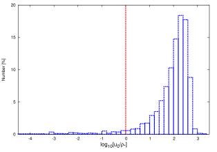
Figure 9: The distribution of $u_{0}/\rho_{\star}$ for the OGLE-III microlensing events. Almost $4.3$ percent of these events are in the range of $u_{0}<\rho_{\star}$. These events are potentially suitable targets for measuring the polarization due to spots on the source star.

We took a perfect circular shape as the source star for the microlensing. In gravitational microlensing the symmetry of source star is broken by producing two distorted images at either side of the lens. This breaking of symmetry causes some phenomena such as the polarization and light centroid shift of source star images. We have showed that there is an orthogonality relation between the polarization and light centroid shift vectors in simple microlensing events. The observations of either polarimetry or astrometry can uniquely indicate the source trajectory on the lens plane. By exploring the sign of impact parameter and source trajectory, all related degeneracies i.e. $u_{0}$ degeneracy, ecliptic degeneracy, parallax-jerk degeneracy and orbiting binary ecliptic degeneracy can be resolved Skowron et al. (2011); Rahvar & Dominik 2009 . We noted that while the polarimetry can probe the small impact parameters, the astrometry is sensitive to the large impact parameters and applying these two observations can probe all the ranges of impact parameter.

In the binary microlensing events, unlike to the simple lensing, the orthogonality between the polarization and centroid shift generally is not valid. During the caustic crossing of the source star which produces the maximum signals of polarization and centroid shift, we studied the behavior of these parameters for the fold and cusp singularities. We have shown that orthogonality relation between the polarization and centroid shift is valid for the fold singularity while this relation is violated in the cusp singularity. This behavior between these two vectors during microlensing events can be an indicator to identify the trajectory of the source with respect to the caustic lines in the binary lensing.

Finally, we have studied the effect of the source spots on polarization, astrometry and photometry of microlensing events for the single lensing. One of features of spots is breaking the orthogonality relation between the polarization and centroid shift. Studying the map of polarization and centroid shift with the photometry provides some information on the physics of the spots on a source star. We have investigated the high magnification events in the list of the OGLE data Wyrzykowski et al. (2014) and show that for $4.3$ percent of events the polarization effect could be enhanced with the amount of about $1$ percent. This means that for a large number of very high magnification microlensing events, the polarimetry follow-up observations can open a new window for studying the stellar spots on various types of stars.

Acknowledgment We are grateful to Philippe Jetzer and Reza Rahimitabar for reading and commenting on the manuscript.

References

- Akitaya et al. (2009) Akitaya H., Ikeda Y., Kawabata K.s., et al., 2009, A & A, 499, L163.
- Agol (1996) Agol E., 1996, MNRAS, 279, L571.
- Blnadford & Narayan (1986) Blnadford R.D., & Narayan R., 1986, ApJ, 310, L568.
- Bogdanov et al. (1996) Bogdanov M. B., Cherepashchuk A. M. & Sazhin M. V., 1996, Ap & SS, 235, L219.
- Chandrasekhar (1960) Chandrasekhar S., 1960, Radiative Transfer. Dover Publications, New York.
- Chang & Refsdal (1979) Chang K., Refsdal S., 1979, Nature, 282, L561.
- Chung et al. (2009) Chung S.-J., Park B.-G., Ryu Y.-H. & Humphrey A. 2009, APJ, 695, L1357.
- Drissen et al. (1989) Drissen L., Bastien P., & St.-Louis N., 1989, ApJ, 97, L814.
- Dominik (1999) Dominik M. 1999, ApJ, 522, L1011.
- Dominik (2004) Dominik M., 2004, MNRAS, 353, L69.
- Einstein (1911) Einstein A. 1911, Annalen der physik, 35, L898.
- Einstein (1936) Einstein A., 1936, Science, 84, L506.
- Gaudi (2012) Gaudi B.s., 2012, A. R. A& A, 50, L411.
- Gaudi & Petters (2002) Gaudi B.S. & Petters A.O., 2002, ApJ, 574, L970.
- Gaudi & Petters (2002) Gaudi B.S. & Petters A.O., 2002, ApJ, 580, L468.
- Gould & Han (2000) Gould A. & Han C. 2000, ApJ, 538, L653.
- Høg et al. (1995) Høg, E., Novikov, I. D., & Polnarev, A. G. 1995, A & A , 294, L287.
- Hayashi et al. (1962) Hayashi C., Hōshi R., Sugimoto D., 1962, Prog. Theor. Phys. Suppl., 22, L1.
- Ingrosso et al. (2012) Ingrosso, G., Calchi Novati,S., De Paolis F., et al. 2012, MNRAS, 426, L1496.
- Jeong et al. (1999) Jeong Y., Han C. & Park S.-H. 1999, ApJ,511, L569.
- Liebes (1964) Liebes, Jr.S., 1964, Phys. Rev., 133, L835.
- Mehrabi & Rahvar (2014) Mehrabi A. & Rahvar S., 2014, In preparation.
- Miralda-Escdé (1996) Miralda-Escudé J., 1996, ApJ, 470, L113.
- Miyamoto & Yoshii (1995) Miyamoto, M. & Yoshii, Y. 1995, AJ, 110, L1427.
- Mao & Witt (1998) Mao S., & Witt H.J., 1998, MNRAS, 300, L1041.
- (26) Paczyński B., 1986a, ApJ, 301, L502.
- (27) Paczyński B., 1986b, ApJ, 304, L1.
- Paczyński (1997) Paczyński B., 1997, Astrophys. J. Lett. astro-ph/9708155.
- Petters & Witt (1996) Petters A. O., & Witt H. J., 1996, J. Math. Phys., 37 L2920.
- Rahvar & Ghassemi (2005) Rahvar, S., & Ghassemi, S. 2005, A & A, 438, L153.
- (31) Rahvar, S., & Dominik, M. 2009, MNRAS, 392, 1193
- Robin et al. (2003) Robin, A. C., et al., 2003, A & A, 409, L523.