Efficient merging of multiple segments of Bézier curves

Abstract

This paper deals with the merging problem of segments of a composite Bézier curve, with the endpoints continuity constraints. We present a novel method which is based on the idea of using constrained dual Bernstein polynomial basis (P. Woźny, S. Lewanowicz, Comput. Aided Geom. Design 26 (2009), 566–579) to compute the control points of the merged curve. Thanks to using fast schemes of evaluation of certain connections involving Bernstein and dual Bernstein polynomials, the complexity of our algorithm is significantly less than complexity of other merging methods.

1 Introduction

This paper deals with the merging problem of segments of a composite Bézier curve, in other words: multiple adjacent Bézier curves, with the endpoints continuity constraints. More specifically, we consider the following approximation problem.

Problem 1.1

[Merging of multiple segments of Bézier curves] Let $0=t_{0}<t_{1}<\ldots<t_{s}=1$ be a partition of the interval $[0,\,1]$. Let be given a composite Bézier curve $P(t)$ ($t\in[0,\,1]$) which in the interval $[t_{i-1},\,t_{i}]$ ($i=1,2,\ldots,s$) reduces to a Bézier curve $P^{i}(t)$ of degree $n_{i}$, i.e.,

$$P(t)=P^{i}(t):=\sum_{j=0}^{n_{i}}p^{i}_{j}\,B^{n_{i}}_{j}\left(\frac{t-t_{i-1}}{\Delta t_{i-1}}\right)\qquad(t_{i-1}\leq t\leq t_{i}),$$ (1.1)

where $\Delta t_{i-1}:=t_{i}-t_{i-1}$, and

$$B^{n}_{j}(t):=\binom{n}{j}t^{j}(1-t)^{n-j}\qquad(0\leq j\leq n)$$

are Bernstein basis polynomials of degree $n$. Find a degree $m$ ($\geq\max_{i}{n_{i}}$) Bézier curve

$$R(t):=\sum_{j=0}^{m}r_{j}\,B^{m}_{j}(t)\qquad(0\leq t\leq 1)$$ (1.2)

such that the error

$$\int_{0}^{1}\|P(t)-R(t)\|^{2}\mbox{${\rm\,d}t$}$$

is minimized in the space $\Pi^{d}_{m}$ of parametric polynomials in $\mathbb{R}^{d}$ of degree at most $m$ (for simplicity, we write $\Pi_{m}:=\Pi^{1}_{m}$) under the additional conditions that

$$\begin{array}[]{l}R^{(i)}(0)=P^{(i)}(0)\qquad(i=0,1,\ldots,k-1),\\[2.15277pt] R^{(j)}(1)=P^{(j)}(1)\qquad(j=0,1,\ldots,l-1),\end{array}$$ (1.3)

where $k\leq n_{1}+1$, $l\leq n_{s}+1$, and $k+l\leq m$. Here $\|\cdot\|$ is the Euclidean vector norm.

There have been many papers relevant to this problem. As for merging of two Bézier curves, besides the pioneering work by Hoschek [3], we should mention papers [4, 8, 10, 11, 13]. Solving problem of merging more than two segments may be reduced to repeated merging of two curves. This, however, may generate loss in accuracy of results and increase of computational cost. The only existing algorithms to solve the problem of merging multiple Bézier adjacent curves are those of [1] and [9]. In the first one, only $C^{0}$ continuity at the endpoints can be imposed, which results in its limited applicability in CAGD. The second algorithm is much more general, accepting $C^{r,s}$ ($r,s\geq 0$) continuity conditions. Notice that the $G^{1}$ multiwise merging also was studied in [9].

We present a novel method which is based on the idea of using constrained dual Bernstein polynomial basis [12] to compute the control points $r_{i}$. Thanks to using fast schemes of evaluation of some connections involving Bernstein and dual Bernstein polynomials, our algorithm is rather efficient. Its complexity is $O(sm^{2})$, which is significantly less than complexity of the methods in [1] and [9].

The outline of this paper is as follows. Section 2 has preliminary character. Section 3 brings a complete solution to Problem 1.1. Section 4 deals with algorithmic implementation of the proposed method. In Section 5, we give some examples showing efficiency of our method. Conclusions are given in Section 6.

2 Preliminaries

Let $\Pi_{m}^{(k,l)}$, where $k$ and $l$ are nonnegative integers such that $k+l\leq m$, be the space of all polynomials of degree at most $m$, whose derivatives of order less than $k$ at $t=0$, as well as derivatives of order less than $l$ at $t=1$, vanish:

$$\Pi_{m}^{(k,l)}:=\left\{P\in\Pi_{m}\>:\>P^{(i)}(0)=0\quad(0\leq i\leq k-1)\;\mbox{and}\;P^{(j)}(1)=0\quad(0\leq j\leq l-1)\right\}.$$

Obviously, $\mbox{dim}\;\Pi_{m}^{(k,l)}=m-k-l+1$, and the Bernstein polynomials $\left\{B^{m}_{k},B^{m}_{k+1},\ldots,B^{m}_{m-l}\right\}$ form a basis of this space. There is a unique dual constrained Bernstein basis of degree $m$ (see, e.g., [5]),

$$D^{(m,k,l)}_{k},D^{(m,k,l)}_{k+1},\ldots,D^{(m,k,l)}_{m-l},$$

satisfying

$$\left\langle D^{(m,k,l)}_{i},\,B^{m}_{j}\right\rangle=\delta_{ij}\qquad(i,j=k,k+1,\ldots,m-l),$$

where $\delta_{ij}$ is 1 if $i=j$ and 0 otherwise, and the inner product $\langle\cdot,\cdot\rangle$ is given by

$$\langle f,\,g\rangle:=\int_{0}^{1}f(t)g(t)\mbox{${\rm\,d}t$}.$$

For $k=l=0$ (the unconstrained case), we have dual Bernstein basis $D^{m}_{i}:=D^{(m,0,0)}_{i}$ ($i=0,1,\ldots,m$) of the space $\Pi_{m}^{(0,0)}=\Pi_{m}$.

Lemma 2.2

Let $n$ and $m$ be positive integers such that $n\leq m$. The following formula holds:

$$B_{i}^{n}(t)=\sum_{j=0}^{m}a_{ij}^{(n,m)}D^{m}_{j}(t)\qquad(0\leq i\leq n;\ n\leq m),$$

where

$$a_{ij}^{(n,m)}:=\frac{1}{m+n+1}\binom{n}{i}\binom{m}{j}\mbox{$\displaystyle\binom{n+m}{i+j}^{\!\!-1}\!\!$}.$$ (2.1)

Proof 1

Obviously, we have

$$a_{ij}^{(n,m)}=\langle B_{i}^{n},B_{j}^{m}\rangle=\int_{0}^{1}B^{n}_{i}(t)B^{m}_{j}(t)\mbox{${\rm\,d}t$},$$

and the result follows by the well known properties of Bernstein polynomials (see, e.g., [2, §6.10]):

$$B^{n}_{i}(t)B^{m}_{j}(t)=\binom{n}{i}\binom{m}{j}\mbox{$\displaystyle\binom{n+m}{i+j}^{\!\!-1}\!\!$}B^{n+m}_{i+j}(t),$$

$$\int_{0}^{1}B^{n+m}_{i+j}(t)\mbox{${\rm\,d}t$}=\frac{1}{n+m+1}.$$

Lemma 2.3

Let $m,k,l\in\mathbb{N}$ be such that $0\leq k+l\leq m$ and let $f$ be a function defined on $[0,\,1]$. The polynomial $S\in\Pi_{m}^{(k,l)}$, which gives minimum value of the norm

$$\|f-S\|_{L_{2}}:=\mbox{$\left\langle{f-S},{f-S}\right\rangle$}^{\frac{1}{2}},$$

is given by

$$S=\sum_{i=k}^{m-l}\mbox{$\left\langle{f},{B^{m}_{i}}\right\rangle$}D^{(m,k,l)}_{i}.$$ (2.2)

Proof 2

Obviously, $S$ has the following representation in the dual Bernstein basis of the space $\Pi_{m}^{(k,l)}$:

$$S=\sum_{i=k}^{m-l}\mbox{$\left\langle{S},{B^{m}_{i}}\right\rangle$}D^{(m,k,l)}_{i}.$$

On the other hand, a classical characterization of the best approximation polynomial $S$ is that $\mbox{$\left\langle{f-S},{Q}\right\rangle$}=0$ holds for any polynomial $Q\in\Pi_{m}^{(k,l)}$. In particular, for $Q=B^{m}_{i}$, we obtain

$$\mbox{$\left\langle{f},{B^{m}_{i}}\right\rangle$}=\mbox{$\left\langle{S},{B^{m}_{i}}\right\rangle$}\qquad(k\leq i\leq m-l).$$

Hence, the formula (2.2) follows.

Further properties of the polynomials $D^{(m,k,l)}_{i}$ are studied in [6, 12] and in the recent paper [7], where the following result is given.

Lemma 2.4 ([7])

The constrained dual basis polynomials have the Bézier-Bernstein representation

$$D^{(m,k,l)}_{i}=\sum_{j=k}^{m-l}c_{ij}(m,k,l)\,B^{m}_{j},$$ (2.3)

where the coefficients $c_{ij}\equiv c_{ij}(m,k,l)$ satisfy the recurrence relation

$$c_{i+1,j}= \frac{1}{A(i)}\,\left\{2(i-j)(i+j-m)\,c_{ij}+B(j)\,c_{i,j-1}+A(j)\,c_{i,j+1}-B(i)\,c_{i-1,j}\right\}$$

$$\hphantom{\frac{1}{A(i)}\,\{+B(j)\,c_{i,j-1}+A(j)\,c_{i,j+1}}(k\leq i\leq m-l-1,\quad k\leq j\leq m-l)$$ (2.4)

with

$$\begin{array}[]{l}A(u):=(u-m)(u-k+1)(u+k+1)/(u+1),\\[8.61108pt] B(u):=u(u-m-l-1)(u-m+l-1)/(u-m-1).\end{array}$$

We adopt the convention that $c_{ij}:=0$ if $i<k$, or $i>m-l$, or $j<k$, or $j>m-l$. The starting values are

$$c_{kj}=(-1)^{j-k}(2k+1)\mbox{$\displaystyle\binom{m}{k}^{\!\!-1}\!\!$}\,\binom{m+k-l+1}{2k+1}\mbox{$\displaystyle\binom{m}{j}^{\!\!-1}\!\!$}\,\binom{m-k-l}{j-k}\binom{m+k+l+1}{k+j+1},$$ (2.5)

where $j=k,k+1,\ldots,m-l$.

In the next section, we will need the following restriction of the representation of the polynomial $B^{m}_{j}$ to a subinterval of the interval $[0,\,1]$.

Lemma 2.5

Let $0=t_{0}<t_{1}<\ldots<t_{s}=1$ be a partition of the interval $[0,\,1]$. In the subinterval $[t_{i-1},\,t_{i}]$ ($i=1,2,\ldots,s$), the Bernstein polynomial $B^{m}_{j}$ can be expressed in the form

$$B^{m}_{j}(t)=\sum_{h=0}^{m}d^{(i)}_{jh}B^{m}_{h}\left(\frac{t-t_{i-1}}{\Delta t_{i-1}}\right),$$ (2.6)

where

$$d^{(i)}_{jh}:=\sum_{v=0}^{h}B^{m-h}_{j-v}(t_{i-1})B^{h}_{v}(t_{i}).$$ (2.7)

Proof 3

The result is obtained in two steps. First, subdivide the polynomial

$$B^{m}_{j}(t)=\sum_{h=0}^{m}\delta_{jh}B^{m}_{h}(t)$$

at the point $t_{i}$ to obtain two forms for the subintervals $[0,\,t_{i}]$ and $[t_{i},\,1]$. Next, subdivide the form corresponding to $[0,\,t_{i}]$ at $t_{i-1}/t_{i}$. We obtain the formula (2.6) with the coefficients $d^{(i)}_{jh}$ given by

$$d^{(i)}_{jh}:=\sum_{w=0}^{m-h}B^{m-h}_{w}(t_{i-1}/t_{i})B^{w+h}_{j}(t_{i})$$

(we ignore the fact that the initial terms of the sum vanish as $B^{w+h}_{j}(t_{i})=0$ for $0\leq w<j-h$). Using the identity

$$B^{n+q}_{j}(x)=\sum_{w=0}^{q}B^{q}_{w}(x)B^{n}_{j-w}(x),$$

which can be easily proved using some basic properties of the Bernstein polynomials (see, e.g., [2, §6.10]), and

$$B^{n}_{j}(cx)=\sum_{v=0}^{n}B^{n}_{v}(x)B^{v}_{j}(c)$$

(ibid.), it can be seen that

$$d^{(i)}_{jh} =\sum_{w=0}^{m-h}B^{m-h}_{w}(t_{i-1}/t_{i})\sum_{v=0}^{h}B^{h}_{v}(t_{i})B^{w}_{j-v}(t_{i})$$

$$=\sum_{v=0}^{h}B^{h}_{v}(t_{i})\sum_{w=0}^{m-h}B^{m-h}_{w}(t_{i-1}/t_{i})B^{w}_{j-v}(t_{i})$$

$$=\sum_{v=0}^{h}B^{h}_{v}(t_{i})B^{m-h}_{j-v}(t_{i-1}).$$

Equation (2.6) is obviously equivalent to

$$B^{m}_{j}(u\Delta t_{i-1}+t_{i-1})=\sum_{h=0}^{m}d^{(i)}_{jh}B^{m}_{h}\left(u\right)\qquad(0\leq u\leq 1).$$ (2.8)

Now, by the bi-orthogonality property of the bases $\{B^{m}_{h}\}$ and $\{D^{m}_{g}\}$, we have

$$d^{(i)}_{jh}=\int_{0}^{1}B^{m}_{j}(u\Delta t_{i-1}+t_{i-1})D^{m}_{h}(u)\mbox{${\rm\,d}u$}.$$ (2.9)

Lemma 2.6

For $i=1,2,\ldots s$, the coefficients $d_{jh}^{(i)}$ satisfy the following recurrence equation:

$$\Delta t_{i-1}\left[(m-j+1)d_{j-1,h}^{(i)}+(2j-m)d_{jh}^{(i)}-(j+1)d_{j+1,h}^{(i)}\right]\\ \qquad\quad=(m-h)d_{j,h+1}^{(i)}+(2h-m)d_{jh}^{(i)}-hd_{j,h-1}^{(i)}\\ (1\leq j\leq m-1;\ 0\leq h\leq m).$$

Proof 4

Differentiate both sides of Equation (2.8) with respect to $u$, and make use of the identity

$$\frac{\mbox{d}}{\mbox{d}u}B^{m}_{j}(u)=(m-j+1)B^{m}_{j-1}(u)+(2j-m)B^{m}_{j}(u)-(j+1)B^{m}_{j+1}(u).$$

Equating the Bézier coefficients gives the result.

3 Merging of the composite Bézier curve segments

Clearly, the Bézier curve being the solution of Problem 1.1 can be obtained in a componentwise way. Hence, it is sufficient to give the details of our method of solving this problem in case where $d=1$.

Theorem 3.7

Let $0=t_{0}<t_{1}<\ldots<t_{s}=1$ be a partition of the interval $[0,\,1]$. Let be given the piecewise polynomial function $P(t)$ ($t\in[0,\,1]$), which in the interval $[t_{i-1},\,t_{i}]$ ($i=1,2,\ldots,s$) reduces to a polynomial $P^{i}(t)$ of degree $n_{i}$, with the Bézier coefficients $p^{i}_{j}$ ($i=1,2,\ldots,s;\;j=0,1,\ldots,n_{i}$) (cf. (1.1)). The coefficients $r_{0},r_{1},\ldots,r_{m}$ of the polynomial (1.2) minimising the error

$$\|R-P\|^{2}_{L_{2}}:=\langle R-P,R-P\rangle$$

with constraints (1.3) are given by

$$\displaystyle r_{j}=\binom{n_{1}}{j}\binom{m}{j}^{\!-1}\,\Delta^{j}p^{1}_{0}-\sum_{h=0}^{j-1}(-1)^{j+h}\binom{j}{h}r_{h}\qquad(j=0,1,\ldots,k-1),$$ (3.1)

$$\displaystyle r_{m-j}=(-1)^{j}\binom{n_{s}}{j}\binom{m}{j}^{\!-1}\,\Delta^{j}p^{s}_{n_{s}-j}-\sum_{h=1}^{j}(-1)^{h}\binom{j}{h}r_{m-j+h}\qquad(j=0,1,\ldots,l-1),$$ (3.2)

$$r_{j}=\sum_{h=k}^{m-l}\hat{r}_{h}c_{hj}(m,k,l)\qquad(j=k,k+1,\ldots,m-l),$$ (3.3)

where

$$\hat{r}_{h} :=\sum_{i=1}^{s}\Delta t_{i-1}\sum_{v=0}^{m}\hat{p}^{i}_{v}d^{(i)}_{hv}-\frac{1}{2m+1}\binom{m}{h}\left(\sum_{v=0}^{k-1}+\sum_{v=m-l+1}^{m}\right)\mbox{$\displaystyle\binom{2m}{h+v}^{\!\!-1}\!\!$}\binom{m}{v}r_{v},$$ (3.4)

$$\hat{p}^{i}_{v} :=\frac{1}{m+n_{i}+1}\binom{m}{v}\sum_{q=0}^{n_{i}}\mbox{$\displaystyle\binom{m+n_{i}}{q+v}^{\!\!-1}\!\!$}\binom{n_{i}}{q}p^{i}_{q},$$ (3.5)

with $c_{hj}(m,k,l)$ and $d^{(i)}_{jh}$ being introduced in (2.3) and (2.7), respectively. Here we use the standard notation $\Delta^{0}c_{h}:=c_{h}$, $\Delta^{j}c_{h}:=\Delta^{j-1}c_{h+1}-\Delta^{j-1}c_{h}$ ($j=1,2,\ldots$).

Proof 5

Recall that for arbitrary polynomial of degree $N$,

$$U_{N}(t)=\sum_{h=0}^{N}u_{h}\,B^{N}_{h}(t),$$

the well-known formulas hold (see, e.g., [2, §5.3])

$$U^{(j)}_{N}(0) = \frac{N!}{(N-j)!}\Delta^{j}u_{0}=\frac{N!}{(N-j)!}\sum_{h=0}^{j}(-1)^{j+h}\binom{j}{h}u_{h},$$

$$U^{(j)}_{N}(1) = \frac{N!}{(N-j)!}\Delta^{j}u_{N-j}=\frac{N!}{(N-j)!}\sum_{h=0}^{j}(-1)^{j+h}\binom{j}{h}u_{N-j+h}.$$

Using the above equations in (1.3), we obtain the forms (3.1) and (3.2) for the coefficients $r_{0},\,r_{1},\ldots,r_{k-1}$ and $r_{m-l+1},\ldots,r_{m-1},r_{m}$, respectively.

The remaining coefficients $r_{k},\,r_{k+1},\,\ldots,\,r_{m-l}$ are to be determined so that

$$\|P-R\|^{2}_{L_{2}}=\|W-S\|^{2}_{L_{2}}$$

has the least value, where

$$W :=P-\left(\sum_{h=0}^{k-1}+\sum_{h=m-l+1}^{m}\right)r_{h}B^{m}_{h},$$

$$S :=\sum_{j=k}^{m-l}r_{j}B^{m}_{j}.$$

To be strict, we first obtain the coefficients $\hat{r}_{j}$ of the searched polynomial in the constrained dual Bernstein basis $\{D^{(m,k,l)}_{h}\}$,

$$S=\sum_{j=k}^{m-l}\hat{r}_{j}D^{(m,k,l)}_{j};$$

then the Bézier coefficients $r_{j}$ of $S$ will be easily computed using Equation (3.3) (cf. Lemma 2.4).

Now, using Lemma 2.2, we represent each segment $P^{i}$ of the original piecewise polynomial $P$ in the dual Bernstein basis of degree $m$,

$$P^{i}(t)=\sum_{v=0}^{m}\hat{p}^{i}_{v}D^{m}_{v}\left(\frac{t-t_{i-1}}{\Delta t_{i-1}}\right)$$

with $\hat{p}^{i}_{v}$ being defined in (3.5).

Using Lemma 2.3 and Equation (2.9), we obtain

$$\hat{r}_{j}= \left<W,B_{j}^{m}\right>=\int_{0}^{1}W(t)B_{j}^{m}(t)\mbox{${\rm\,d}t$}$$

$$= \sum_{i=1}^{s}\sum_{h=0}^{m}\hat{p}^{i}_{h}\int_{t_{i-1}}^{t_{i}}D_{h}^{m}\left(\frac{t-t_{i-1}}{\Delta t_{i-1}}\right)B_{j}^{m}(t)\mbox{${\rm\,d}t$}$$

$$\hphantom{sum_{i=1}^{s}}-\left(\sum_{h=0}^{k-1}+\sum_{h=m-l+1}^{m}\right)r_{h}\int_{0}^{1}B_{h}^{m}(t)B_{j}^{m}(t)\mbox{${\rm\,d}t$}$$

$$= \sum_{i=1}^{s}\sum_{h=0}^{m}\hat{p}^{i}_{h}\Delta t_{i-1}\int_{0}^{1}D_{h}^{m}(u)B_{j}^{m}(\Delta t_{i-1}u+t_{i-1})\mbox{${\rm\,d}u$}$$

$$\hphantom{sum_{i=1}^{s}}-\left(\sum_{h=0}^{k-1}+\sum_{h=m-l+1}^{m}\right)r_{h}\frac{1}{2m+1}\binom{m}{h}\binom{m}{j}\mbox{$\displaystyle\binom{2m}{h+j}^{\!\!-1}\!\!$}$$

$$= \sum_{i=1}^{s}\Delta t_{i-1}\sum_{h=0}^{m}\hat{p}^{i}_{h}d_{jh}^{(i)}-\frac{1}{2m+1}\binom{m}{j}\left(\sum_{h=0}^{k-1}+\sum_{h=m-l+1}^{m}\right)r_{h}\binom{m}{h}\mbox{$\displaystyle\binom{2m}{h+j}^{\!\!-1}\!\!$}$$

$$\hphantom{sum_{i=1}^{s}\sum_{h=0}^{m}\hat{p}^{i}_{h}\int_{t_{i-1}}^{t_{i}}D_{h}^{m}\left(\frac{t-t_{i-1}}{\Delta t_{i-1}}\right)B_{j}^{m}(t)\mbox{${\rm\,d}t$}}(j=k,k+1,\ldots,m-l).$$

This completes the proof.

Now, let the composite curve $P$ and the merged curve $R$ be curves in $\mathbb{R}^{d}$ ($d\geq 1$). Let $p^{i}_{j}=(p^{i}_{j1},p^{i}_{j2},\ldots,p^{i}_{jd})$ ($i=1,2,\ldots,s;\ j=0,1,\ldots,n_{i}$), and $r_{j}=(r_{j1},r_{j2},\ldots,r_{jd})$ ($j=0,1,\ldots,m$) be the control points of $P$ and $R$, respectively. For $i=1,2,\ldots,s$ and $h=1,2,\ldots,d$, let us define vectors

$$\pi^{i}_{h}:= \left[p^{i}_{0h},p^{i}_{1h},\ldots,p^{i}_{n_{i},h}\right]\in\mathbb{R}^{n_{i}+1},$$

$$\varrho^{i}_{h}:= \left[\varrho^{i}_{0h},\varrho^{i}_{1h},\ldots,\varrho^{i}_{mh}\right]\in\mathbb{R}^{m+1},$$

where

$$\varrho^{i}_{zh}:=\sum_{j=0}^{m}r_{jh}d^{(i)}_{jz}\qquad(z=0,1,\ldots,m).$$ (3.6)

It can be shown that the $L_{2}$-distance between the curves $P$ and $R$ is given by the formula:

$$E_{2}:= \|P-R\|_{L_{2}}$$

$$= \left(\sum_{i=1}^{s}\Delta t_{i-1}\sum_{h=1}^{d}\left[I_{n_{i},n_{i}}(\mathbf{\pi}^{i}_{h},\mathbf{\pi}^{i}_{h})-2I_{n_{i},m}(\mathbf{\pi}^{i}_{h},\mathbf{\varrho}^{i}_{h})+I_{mm}(\mathbf{\varrho}^{i}_{h},\mathbf{\varrho}^{i}_{h})\right]\right)^{\frac{1}{2}},$$ (3.7)

where

$$I_{NM}(u,v):=\sum_{j=0}^{N}u_{j}\sum_{z=0}^{M}a_{jz}^{(N,M)}v_{z},$$

with $u:=\left[u_{0},u_{1},\ldots,u_{N}\right]$ and $v:=\left[v_{0},v_{1},\ldots,v_{M}\right]$, the notation used being that of (2.1).

4 Algorithms

4.1 Auxiliary computations

In this section, we discuss details of algorithmic implementation of the results given in Theorem 3.7. First, we have to precompute efficiently the coefficients $c_{ij}(m,k,l)\;$ introduced in Lemma 2.4 (see Table 1).

$$\begin{array}[]{cccccc}&0&0&\ldots&0&\\ 0&c_{kk}&c_{k,k+1}&\ldots&c_{k,m-l}&0\\ 0&c_{k+1,k}&c_{k+1,k+1}&\ldots&c_{k+1,m-l}&0\\ \lx@intercol\dotfill\hfil\hfil\lx@intercol\\ 0&c_{m-l,k}&c_{m-l,k+1}&\ldots&c_{m-l,m-l}&0\\ &0&0&\ldots&0&\end{array}$$

Table 1: The $c$-table

Now, the table can be completed easily by using formulas (2.4), (2.5) (cf. [7, Algorithm 3.3]), with the complexity $O(m^{2})$.

Another task is to evaluate all the coefficients $d_{jh}^{(i)}$ ($i=1,2,\ldots,s;\ j=0,1,\ldots,m;\ h=0,1,\ldots,m$) (cf. (2.7)). Thanks to Lemma 2.6, we can do it using the following algorithm.

Algorithm 4.8

​[Evaluation of the coefficients $d_{jh}^{(i)}$]
Input: $m$, $s$, $0=t_{0}<t_{1}<\ldots<t_{s}=1$
Output: table of the coefficients $d_{jh}^{(i)}\ (i=1,2,\ldots,s;\ j=0,1,\ldots,m;\ h=0,1,\ldots,m)$

Step 1.

For $i=1,2,\ldots,s$, compute

$$d_{-10}^{(i)}:=0,\quad d_{00}^{(i)}:=(1-t_{i-1})^{m},$$

$$d_{-1h}^{(i)}:=0,\quad d_{0h}^{(i)}:=\frac{1-t_{i}}{1-t_{i-1}}d_{0,h-1}^{(i)}\qquad(h=1,2,\ldots,m).$$

Step 2.

For $i=1,2,\ldots,s$, $j=0,1,\ldots,m-1$, and $h=0,1,\ldots,m$, compute

$$d_{j+1,h}^{(i)}:= (j+1)^{-1}\left\{\left(\Delta t_{i-1}\right)^{-1}\left[hd_{j,h-1}^{(i)}-(2h-m)d_{jh}^{(i)}-(m-h)d_{j,h+1}^{(i)}\right]\right.$$

$$\hphantom{(j+1)^{-1}\{}\left.+(m-j+1)d_{j-1,h}^{(i)}+(2j-m)d_{jh}^{(i)}\right\}.$$

Observe that complexity of Algorithm 4.8 is $O(sm^{2})$.

4.2 Main algorithm

Now, the presented method of merging of segments of a composite Bézier curve is summarized in the following algorithm.  

Algorithm 4.9

[Merging of segments of a composite Bézier curve]
Input: $p^{i}_{j}\ (j=0,1,\ldots,n_{i})$, $n_{i}\ (i=1,2,\ldots,s)$,
Input: $m$, $k$, $l$, $0=t_{0}<t_{1}<\ldots<t_{s}=1$
Output: solution $r_{0},r_{1},\dots,r_{m}$ of the Problem 1.1, and its error $E_{2}$

Step 1.

Compute $r_{0},r_{1},\ldots,r_{k-1}$ by (3.1).

Step 2.

Compute $r_{m-l+1},r_{m-l+2},\ldots,r_{m}$ by (3.2).

Step 3.

Compute $\hat{p}^{i}_{j}\ (i=1,2,\ldots,s;\ j=0,1,\ldots,m)$ by (3.5).

Step 4.

Compute $d_{jh}^{(i)}$ for $i=1,2,\ldots,s$; $j=0,1,\ldots,m$; $h=0,1,\ldots,m$, using Algorithm 4.8.

Step 5.

Compute $\hat{r}_{j}\ (j=k,k+1,\ldots,m-l)$ by (3.4).

Step 6.

Compute $c_{ij}(m,k,l)$ for $i,j=k,k+1,\ldots,m-l$, using (2.4), (2.5) (cf. [7, Algorithm 3.3]).

Step 7.

Compute $r_{j}\ (j=k,k+1,\ldots,m-l)$ by (3.3).

Step 8.

Compute $\varrho^{i}_{zh}\ (i=1,2,\ldots,s;\ z=0,1,\ldots,m;\ h=1,2,\ldots,d)$ by (3.6).

Step 9.

Compute $E_{2}$ by (3.7).

Notice that complexity of Algorithm 4.9 is $O(sm^{2})$.

5 Examples

In this section, we give several examples of using Algorithm 4.9. In every case we give the $L_{2}$-error $E_{2}$ as well as the maximum error

$$E_{\infty}:=\max_{t\in D_{N}}\|P(t)-R(t)\|\approx\max_{t\in[0,1]}\|P(t)-R(t)\|,$$

where $D_{N}:=\left\{0,1/N,2/N,\ldots,1\right\}$ with $N=500$. Generalizing the approach of [8, (6.1)], partition of the interval $[t_{0},t_{s}]=[0,\,1]$ is determined according to the lengths of segments $P^{i}$:

$$t_{j}:=L_{j}/L_{s}\qquad(j=1,2,\ldots,s-1),$$ (5.1)

where

$$L_{q}:=\sum_{i=1}^{q}\int_{0}^{1}\left\|\frac{\mbox{${\rm\,d}$}}{\mbox{${\rm\,d}t$}}\sum_{h=0}^{n_{i}}p^{i}_{h}B^{n_{i}}_{h}(t)\right\|\mbox{${\rm\,d}t$}.$$

Integrals are evaluated using the $\mbox{Maple}^{TM}13$ function int with the option numeric.

Results of the experiments have been obtained on a computer with Intel Core i5-3337U 1.8GHz processor and 8GB of RAM, using $32$-digit arithmetic. Notice that $\mbox{Maple}^{TM}13$ worksheet containing programs and tests can be found on the webpage webpage http://www.ii.uni.wroc.pl/~pgo/papers.html.

Example 5.10

We use Algorithm 4.9 to merge the composite curve ’’Ampersand‘‘, with three fifth degree Bézier segments, defined by the control points $\{(1.09,0.03),$ $(1.02,0.21),$ $(0.6,0.75),$ $(0.5,1.11),$ $(0.85,1.12),$ $(0.93,1.03)\}$, $\{(0.93,1.03),$ $(1.01,0.96),$ $(1.02,0.76),$ $(0.8,0.65),$ $(0.62,$
$0.38),$ $(0.61,0.23)\}$, and $\{(0.61,0.23),$ $(0.59,0.1),$ $(0.67,0.02),$ $(0.91,-0.05),$ $(1.12,0.05),$ $(1.08,$
$0.22)\}$, respectively. According to (5.1), we have $t_{0}=0,\ t_{1}\doteq 0.45,\ t_{2}\doteq 0.76,\ t_{3}=1$. Obtained results are given in Table 2. Moreover, we give the comparison of running times required to compute the resulting control points. Clearly, our method is faster than the one presented in [9]. Figures 1a and 1b illustrate the results for two representative cases. This example shows that merging may result in data compression.

Parameters				Errors			Running times [ms]
$m$	$k$	$l$		$E_{2}$	$E_{\infty}$		Algorithm 4.9	Lu [9]
$8$	$2$	$1$		$8.57E{-}3$	$2.36E{-}2$		$10$	$85$
	$2$	$2$		$1.99E{-}2$	$5.46E{-}2$		$11$	$87$
	$3$	$2$		$3.89E{-}2$	$1.04E{-}1$		$10$	$77$
$10$	$2$	$1$		$3.49E{-}3$	$1.32E{-}2$		$16$	$121$
	$2$	$2$		$9.43E{-}3$	$3.36E{-}2$		$15$	$108$
	$3$	$2$		$1.98E{-}2$	$6.08E{-}2$		$15$	$104$
$12$	$2$	$1$		$2.70E{-}3$	$9.84E{-}3$		$22$	$167$
	$2$	$2$		$5.71E{-}3$	$2.29E{-}2$		$22$	$160$
	$3$	$2$		$1.06E{-}2$	$3.81E{-}2$		$19$	$158$

Table 2: Least-squares and maximum errors for merging of three segments of the composite Bézier curve with constraints.

(a)

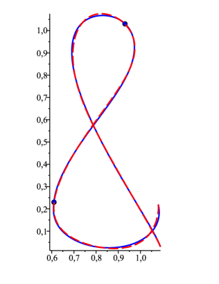
(b)

Figure 1: Merging of three segments of the composite Bézier curve. Original curve (blue solid line) and merged curve (red dashed line) with parameters: (a) $m=10$, $k=3$, $l=2$, and (b) $m=12$, $k=3$, $l=2$.

Example 5.11

The curve ’’Penguin‘‘ is formed by two composite Bézier curves. The left curve has four cubic segments, with the control points $\{(0.31,0.23),$ $(0.35,0.19),$ $(0.39,0.23),$ $(0.37,0.26)\}$, $\{(0.37,0.26),$ $(0.21,0.54),$ $(0.53,0.77),$ $(0.21,0.76)\}$, $\{(0.21,0.76),$ $(0.1,0.76),$ $(0.5,$
$0.88),$ $(0.42,0.79)\}$, and $\{(0.42,0.79),$ $(0.26,0.76),$ $(0.23,0.92),$ $(0.34,0.94)\}$, respectively. The right curve is composed of three cubic segments having control points $\{(0.34,0.94),$ $(0.74,0.99),$ $(0.67,0.19),$ $(0.56,0.21)\}$, $\{(0.56,0.21),$ $(0.19,0.32),$ $(0.62,1.05),$ $(0.56,0.61)\}$, and $\{(0.56,0.61),$ $(0.5,0.24),$ $(0.41,0.41),$ $(0.5,0.64)\}$, respectively. Formula (5.1) gives $t_{0}=0,\ t_{1}\doteq 0.08,\ t_{2}\doteq 0.55,\ t_{3}\doteq 0.78,\ t_{4}=1$ for the left curve, and $t_{0}=0,\ t_{1}\doteq 0.42,\ t_{2}\doteq 0.78,\ t_{3}=1$ for the right one. Results of separate merging of segments of both curves can be seen in Table 3. Two selected cases are shown on Figures 2a and 2b.

Left curve										Right curve
$m$		$k$		$l$		$E_{2}$		$E_{\infty}$		$m$		$k$		$l$		$E_{2}$		$E_{\infty}$
$12$		$1$		$1$		$7.45E{-}3$		$1.90E{-}2$		$10$		$1$		$1$		$1.28E{-}2$		$3.51E{-}2$
		$1$		$2$		$1.05E{-}2$		$2.69E{-}2$				$2$		$1$		$1.28E{-}2$		$3.48E{-}2$
		$2$		$1$		$7.85E{-}3$		$1.93E{-}2$				$1$		$2$		$1.29E{-}2$		$3.49E{-}2$
		$2$		$2$		$1.10E{-}2$		$2.85E{-}2$				$2$		$2$		$1.30E{-}2$		$3.44E{-}2$
$13$		$1$		$1$		$6.68E{-}3$		$1.45E{-}2$		$12$		$1$		$1$		$9.01E{-}3$		$3.00E{-}2$
		$1$		$2$		$7.80E{-}3$		$1.64E{-}2$				$2$		$1$		$1.02E{-}2$		$3.27E{-}2$
		$2$		$1$		$7.28E{-}3$		$1.48E{-}2$				$1$		$2$		$1.14E{-}2$		$2.98E{-}2$
		$2$		$2$		$8.53E{-}3$		$1.71E{-}2$				$2$		$2$		$1.23E{-}2$		$3.25E{-}2$
$14$		$1$		$1$		$4.39E{-}3$		$1.19E{-}2$		$13$		$1$		$1$		$8.65E{-}3$		$2.83E{-}2$
		$1$		$2$		$4.51E{-}3$		$1.27E{-}2$				$2$		$1$		$9.16E{-}3$		$2.81E{-}2$
		$2$		$1$		$4.86E{-}3$		$1.17E{-}2$				$1$		$2$		$1.11E{-}2$		$2.98E{-}2$
		$2$		$2$		$5.08E{-}3$		$1.30E{-}2$				$2$		$2$		$1.16E{-}2$		$2.98E{-}2$

Table 3: Least-squares and maximum errors for separate merging of segments of two composite Bézier curves with constraints.

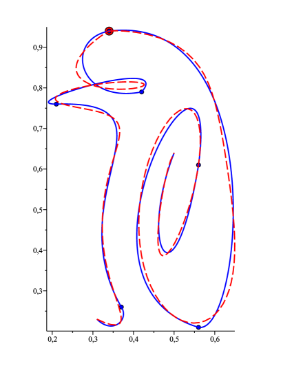
(a)

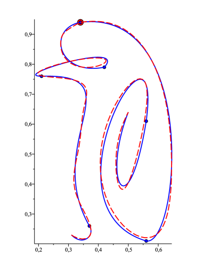
(b)

Figure 2: Separate merging of segments of two composite Bézier curves with constraints. Original curves (blue solid line) and merged curves (red dashed line). (a) Left curve: $m=12$, $k=1$, $l=2$; right curve: $m=10$, $k=2$, $l=1$. (b) Left curve: $m=14$, $k=2$, $l=2$; right curve: $m=13$, $k=2$, $l=2$.

6 Conclusions

We have proposed a novel approach to the problem of merging of multiple adjacent Bézier curves, with the endpoints continuity constraints. We have shown that, contrary to some earlier opinions [9], it is possible to generalize dual Bernstein polynomials approach to compute the control points of the merged curve. Thanks to using fast schemes of evaluation of certain connections involving Bernstein and dual Bernstein polynomials, the complexity of our algorithm is $O(sm^{2})$, which should be compared to the complexity $O(sm^{3})$ of the existing multiple merging methods [1, 9].

As for our future work, we plan to study the above merging problem with $G^{k,l}$ continuity constraints.

References

• [1] M. Cheng, G. Wang, Approximate merging of multiple Bézier segments, Progress in Natural Science 18 (2008), 757–762.
• [2] G. E. Farin, Curves and Surfaces for Computer-Aided Geometric Design. A Practical Guide, fifth edition, Academic Press, Boston, 2002.
• [3] J. Hoschek, Approximate conversion of spline curves, Computer Aided Geometric Design 4 (1987), 59–66.
• [4] S. Hu, R. Tong, T. Ju, J. Sun, Approximate merging of a pair of Bézier curves, Computer-Aided Design 33 (2001), 125–136.
• [5] B. Jüttler, The dual basis functions for the Bernstein polynomials, Advances in Computational Mathematics 8 (1998), 345–352.
• [6] S. Lewanowicz, P. Woźny, Multi-degree reduction of tensor product Bézier surfaces with general constraints, Applied Mathematics and Computation 217 (2011), 4596–4611.
• [7] S. Lewanowicz, P. Woźny, Bézier representation of the constrained dual Bernstein polynomials, Applied Mathematics and Computation 218 (2011), 4580–4586.
• [8] L. Lu, An explicit method for $G^{3}$ merging of two Bézier curves, Journal of Computational and Applied Mathematics 260 (2014), 421–433.
• [9] L. Lu, Explicit algorithms for multiwise merging of Bézier curves, Journal of Computational and Applied Mathematics 278 (2015), 138–148.
• [10] L. Lu, Effective $C^{1}G^{2}$-merging of Two Bézier Curves by Matrix Computation, International Journal of Advancements in Computing Technology 5 (2013), 1117–1123.
• [11] C. Tai, S. Hu, Q. Huang, Approximate merging of B-spline curves via knot adjustment and constrained optimization, Computer-Aided Design 35 (2003), 893–899.
• [12] P. Woźny, S. Lewanowicz, Multi-degree reduction of Bézier curves with constraints, using dual Bernstein basis polynomials, Computer Aided Geometric Design 26 (2009), 566–579.
• [13] P. Zhu, G. Wang, Optimal approximate merging of a pair of Bézier curves with $G^{2}$-continuity, Journal of Zhejiang University SCIENCE A 10 (2009), 554–561.