Molecular Cluster Perturbation Theory. I. Formalism

Abstract

We present second-order molecular cluster perturbation theory (MCPT(2)), a linear scaling methodology to calculate arbitrarily large systems with explicit calculation of individual wavefunctions in a coupled-cluster framework. This new MCPT(2) framework uses coupled-cluster perturbation theory and an expansion in terms of molecular dimer interactions to obtain molecular wavefunctions that are infinite-order in both the electronic fluctuation operator and all possible dimer (and products of dimers) interactions. The MCPT(2) framework has been implemented in the new SIA/Aces4 parallel architecture, making use of the advanced dynamic memory control and fine grained parallelism to perform very large explicit molecular cluster calculations. To illustrate the power of this method, we have computed energy shifts, lattice site dipole moments, and harmonic vibrational frequencies via explicit calculation of the bulk system for the polar and non-polar polymorphs of solid hydrogen fluoride. The explicit lattice size (without using any periodic boundary conditions) was expanded up to 1,000 HF molecules, with 32,000 basis functions and 10,000 electrons. Our obtained HF lattice site dipole moments and harmonic vibrational frequencies agree well with the existing literature.

I Introduction

There are at least two fundamental challenges in modern quantum chemistry: the efficient calculation of both dynamic and static correlation simultaneously, and the calculation of successively larger systems. Diverse classes of methods exist flocke2004 ; tomasi2005 ; gordon2007 ; fedorov2012 ; klamt2011 ; vreven2006 ; podeszwa2008 ; mayhall2011 ; knizia2012 to describe large systems within a quantum mechanical framework by subdivision into smaller fragments. For an overarching summary of modern fragmentation methods, we refer to the review article of Gordon et al. gordon2012 In general, when presented with a large number of degrees of freedom, one has the choice to represent them implicitly or explicitly. Examples of implicit representation include employing periodic boundary conditions or approximating the surrounding system as a bath with a continuum representation. Explicit representations of high numbers of degrees of freedom typically require sub-partitioning of the system in some manner to reduce the computational cost. Our goal in this work is to create an explicit method of handling large systems with a rigorously defined perturbation expansion. We consider it highly desirable to have an explicit model. Inherent to periodic boundary conditions or implicit solvation models is a requirement of homogeneity. Inherently heterogeneous phenomena, such as crystalline defects, solvents with varied electrical moments over the molecule (like carboxylic acids), or surface interactions require some explicit representation of these degrees of freedom.

If we consider an arbitrarily large system consisting of $N$ non-interacting (infinitely separated) molecular clusters, collectively referred to as monomers, we can write the Schrödinger equation for each monomer $X$ as

$$\hat{H}_{X}|\phi_{X}\rangle=E_{X}|\phi_{X}\rangle$$ (1)

where $|\phi_{X}\rangle$ is the properly anti-symmetric monomer wavefunction. The total system’s wavefunction is then a simple direct product of the monomer wavefunctions

$$|\Psi_{p}\rangle=|\phi_{1}\rangle\otimes|\phi_{2}\rangle\otimes\dots|\phi_{N}\rangle.$$ (2)

Assuming that these monomers retain their identity to a large degree as they begin to interact (by adiabatically bringing them to some finite separation), then we can preserve the product nature of the system wavefunction by introducing the complete anti-symmetrizer $\hat{A}$ so that

$$|\Psi\rangle=\hat{A}|\Psi_{p}\rangle=\hat{A}|\phi_{1}\rangle\otimes|\phi_{2}\rangle\otimes|\phi_{3}\rangle\otimes\dots|\phi_{N}\rangle.$$ (3)

The anti-symmetrizer $\hat{A}$ can be written in terms of the permutation operator $\hat{P}$ as

$$\hat{A}=1+\hat{P}$$ (4)

where $\hat{P}$ acting on an electronic wavefunction interchanges electrons between monomers in all possible ways resulting in a completely anti-symmetric wavefunction. This product wavefunction is a common Ansatz in molecular and condensed matter physics distinguished by the various treatments of the anti-symmetrizer and Hamiltonian approximations. By further assuming that each monomer interacts non-covalently with neighboring monomers, the problem becomes an excellent candidate for an intermolecular force expansion buckingham1967 . Using the product wavefunction Eq. 2 as our monomer fermi vacuum, with the specification that the monomer wavefunctions $|\phi_{X}\rangle$ are the Hartree-Fock solutions to Eq. 1, we can write the system electronic Hamiltonian without further approximation as the sum of individual monomer and dimer Hamiltonians,

$$\hat{H}=\sum^{N}_{X}\hat{H}_{X}+\sum^{N}_{X,Y\neq X}\hat{H}_{XY},$$ (5)

where $N$ is the total number of monomers. This exact separation of the Hamiltonian into only monomer and dimer spaces arises from the precisely block diagonal nature of the product wavefunction in Eq. 2, due to approximating the global anti-symmetrizer as $\hat{A}\simeq 1$. Neglecting the global anti-symmetrizer in Eq. 3 like this leads to the well known polarization expansion, whereas the term including $\hat{P}$ leads to the exchange expansion, the details of both expansions are well-documented rybak1991 ; jeziorski1994 .

Traditional methods based on Eq. 3 (such as polarization chalasinski1977 ; jeziorski1994 or symmetry-adapted perturbation theory rybak1991 ; jeziorski1994 ) compute the wavefunction and energy components perturbatively from these two expansions in terms of polarization, induction, dispersion, exchange, and “mixed” terms (see Rybak et al. rybak1991 for a comprehensive discussion). The standard approaches to the intermolecular force perturbation expansion suffer from several significant drawbacks; the expansion in terms of the intermonomer electrostatic operator is nonconvergent and requires explicit inclusion of many-body intermonomer effects lotrich1997 ; cvitas2007 . Also absent in most standard intermolecular expansions is an explicit monomer wavefunction. This lack of a monomer wavefunction greatly hampers the evaluation of solvation shifted or bulk limit properties. It is our goal in this work to address some of the limitations found in traditional methods by developing a monomer centric wavefunction theory that self consistently includes the perturbative effects of the surrounding system.

The success of coupled-cluster (CC) theory bartlett2007 as a rapidly converging description of dynamic correlation makes it a natural candidate for molecular cluster interactions. The behavior of CC theory is the driving force behind many embedding methods flocke2004 ; cammi2009 ; mayhall2011 ; bygrave2012 ; list2014 . Such molecular clusters are dominated by weaker intermolecular forces and are therefore the most amenable to an intermolecular expansion. We present a new infinite-order pairwise-based embedding framework, which we refer to as molecular cluster perturbation theory (MCPT), as a means to efficiently compute the Schrödinger equation for large systems of interacting molecular clusters. The MCPT method combines the coupled-cluster perturbation theory bartlett2010 (CCPT) with the intermolecular force approach buckingham1967 ; jeziorski1994 of products of monomer wavefunctions. By expanding the perturbation series in terms of both the intramolecule (monomer) and intermolecular (dimer) electron fluctuation operators, a formally consistent perturbation theory can be obtained that has many significant advantages.

1. Expanding in terms of pairwise interactions reduces the extremely high computational cost of $O(N^{6}o^{2}v^{4})$ inherent to the standard coupled-cluster theory with all singles and doubles purvis1982 (CCSD) to $O(N^{2}o^{2}v^{4})$ where $o$ ($v$) is the number of occupied (virtual) orbitals of an individual monomer while $N$ is the total number of monomers. Further physical arguments based on the distance scaling of intermolecular forces allow the introduction of a cutoff radius past which all explicit interactions are neglected. This cutoff reduces the MCPT computational scaling to be linear with respect to the number of monomers.

2. Choosing the particle excitation rank partitioning grabouski2007 ; bartlett2010 of the Hamiltonian ($\hat{H}=\hat{H}_{0}+\hat{V}$), the single and double excitation cluster operators (monomer and dimer) completely decouple at first-order in $\hat{V}$ while remaining infinite order in $\hat{H}_{0}$.

3. By our choice of $H_{0}$, all intermolecular interactions are iterated over so that the final monomer wavefunction contains all possible pairwise interactions and products of pairwise interactions to infinite-order. This alleviates the non-convergent nature found in other intermolecular force theories.

4. We neglect the global anti-symmetrization of the total system’s wavefunction by approximating it as a product state of individual monomer wavefunctions.

5. The explicit monomer wavefunction nature of the MCPT formalism allows the further computation of monomer-only properties while retaining the information of the surrounding system. Knowledge of the monomer wavefunctions allows the computation of any quantum mechanical observable (e.g. optical spectra) and the shifts to the observable due to the surrounding system (such as solvation shifts or crystal field effects.

Due to the greatly improved computational scaling, the MCPT framework allows for the calculation of large systems cheaply and explicitly without any continuum representation or periodic boundary conditions. In this work, we report the study of 1,000 hydrogen fluoride molecules in two different crystal polymorphs. This is one of the largest explicit quantum calculations on record, done on merely $\sim 256$ processors within a 12 hour queue.

The HF lattice is one of the simplest systems to describe physically due to the small number of electrons and non-covalent interaction between HF molecules. In the field of calculating correlated wavefunctions for crystalline systems, new methods need simple systems against which to compare to understand the merits of new many-body methodologies. We consider the HF lattice to be a good candidate as a prototype benchmark system. The HF lattice is additionally of theoretical interest as it is not currently known what crystal polymorph is most stable between polar and non-polar forms atoji1954 ; johnson1975 ; otto1986 ; panas1993 ; berski1998 ; buth2004 ; buth2006 ; sode2010 ; bygrave2012 . Work toward this goal is an interesting challenge for new methods, given that previous estimates suggest that the difference between polymorphs at a few kcal/mol. The computational vibrational spectra also poses a challenge for new correlated wavefunction crystal methods as the crystal induced shifts of the IR and Raman spectra are tremendous kittelberger1967 ; anderson1980 ; pinnick1989 ; sode2009 ; sode2012 .

This manuscript is organized as follows: In Sec. II.1 a brief overview of coupled-cluster perturbation theory and the particle rank partitioning of $\hat{H}_{0}$ is presented. This is followed by Sec. II.2 where the derivation and use of the effective molecular cluster Hamiltonians in the CCPT framework is summarized. Working MCPT(2) spin-adapted equations, with other supporting equations, are given in Sec. II.3. After a brief summary of the electronic structure calculations in Sec. III, we present in Sec. IV.1 our large scale calculations on the $10\times 10\times 10$ square HF crystal. Sec. V contains our concluding remarks.

II Molecular Cluster Perturbation Theory

II.1 Second-order coupled cluster perturbation theory and choice of $\hat{H}_{0}$

The CCPT expansion is outlined in detail in this section so that we can build upon the formal definitions later to construct the MCPT equations. For a generic system the Schrödinger equation can be written in terms of the coupled-cluster (CC) exponential expansion as,

$$\hat{H}e^{\hat{T}}|\phi_{0}\rangle=Ee^{\hat{T}}|\phi_{0}\rangle$$ (6)

where the cluster operator, $\hat{T}$, acting on the reference $|\phi_{0}\rangle$ creates $n$-fold excited determinants. The Hamiltonian, $\hat{H}$, is given in normal-ordered second-quantized form as

$$\hat{H}= \langle 0|\hat{H}|0\rangle+\sum_{pq}f^{p}_{q}\{\hat{p}^{\dagger}\hat{q}\}+\frac{1}{4}\sum_{pqrs}\bar{v}^{pq}_{rs}\{\hat{p}^{\dagger}\hat{q}^{\dagger}\hat{s}\hat{r}\}$$ (7)

$$= \langle 0|\hat{H}|0\rangle+\hat{F}+\hat{W}$$ (8)

where $f$ is the usual one particle Fock matrix, $\bar{v}$ are anti-symmetric two-electron integrals and $\{\}$ denotes normal ordering of the included operators. The Hamiltonian can be formally partitioned as a sum of operators $\hat{H}_{0}$ and $\hat{V}$, where

$$\hat{H}_{0}|\phi_{0}\rangle=E_{0}|\phi_{0}\rangle$$ (9)

and

$$\hat{V}\equiv\hat{H}-\hat{H}_{0}$$ (10)

is treated as a perturbation. Writing Eq. 6 and the partitioned Hamiltonian from Eq. 9 we have

$$\left(\hat{H}_{0}+\hat{V}\right)e^{\hat{T}}|\phi_{0}\rangle=Ee^{\hat{T}}|\phi_{0}\rangle.$$ (11)

From here it is possible to obtain the cluster amplitudes and final energy through projection against the appropriate excitation space. Performing the standard similarity transformation,

$$e^{-\hat{T}}\left(\hat{H}_{0}+\hat{V}\right)e^{\hat{T}}|\phi_{0}\rangle=E|\phi_{0}\rangle,$$ (12)

the energy is obtained by projection with the reference space

$$\langle\phi_{0}|e^{-\hat{T}}\left(\hat{H}_{0}+\hat{V}\right)e^{\hat{T}}|\phi_{0}\rangle=E\langle\phi_{0}|\phi_{0}\rangle$$ (13)

while the cluster amplitudes are defined by projecting with the excited manifold $|\phi^{g}\rangle\langle\phi^{g}|$ giving

$$\langle\phi^{g}|e^{-\hat{T}}\left(\hat{H}_{0}+\hat{V}\right)e^{\hat{T}}|\phi_{0}\rangle=0$$ (14)

where $\langle\phi^{g}|$ indicates a $g$-fold excited determinant. The cluster operator $\hat{T}$ can be expanded in the perturbation $\hat{V}$, leading to the CCPT equations for the first-order amplitudes and second-order energy:

$$\langle\phi^{g}|\hat{V}+\left[\hat{H}_{0},\hat{T}\right]|\phi_{0}\rangle=0$$ (15)

$$\langle\phi_{0}|\left[\hat{V},\hat{T}\right]|\phi_{0}\rangle=E^{(2)}.$$ (16)

It is customary to choose $\hat{H}_{0}$ to be the one-particle Fock operator $\hat{F}$, commonly referred to as the Møller-Plesset partitioning. This leads to the standard MPn equations shavitt2009 which have been quintessential to modern computational chemistry. However, other choices in partitioning of the Hamiltonian are possible. In this work we will use the particle rank partitioning,

$$\hat{H}_{0}=\hat{F}^{[0]}+\hat{W}^{[0]},$$ (17)

used in our previous work bartlett2010 ; byrd2014-b where $[0]$ denotes only particle excitation rank conserving contributions. This choice has the advantages over the MPn series that at second-order in the energy (Eq. 16), the singles and doubles amplitude equations from Eq. 15 are linear in the cluster operator $\hat{T}$ and completely decoupled from each other (as contrasted with the standard CCSD theory, which introduces significant coupling between the singles and doubles cluster amplitudes). From this definition of $\hat{H}_{0}$, the perturbation

$$\hat{V}=\hat{H}-\hat{H}_{0}=\hat{F}^{[\pm 1]}+\hat{W}^{[\pm 1,\pm 2]}$$ (18)

will contain all terms that do not preserve particle excitation rank (see Fig. 1 for the diagrammatic forms of the $\hat{F}^{[n]}$ and $\hat{W}^{[n]}$ operators).

If we use canonical Hartree-Fock orbitals in our reference wavefunction $|\phi_{0}\rangle$, with the choice of $\hat{H}_{0}$ defined above, the first-order amplitudes and second-order energy are equivalent to LCCD (linear coupled-cluster theory). However, as will be illustrated below, for non-Hartree-Fock orbitals this LCCD amplitude and energy equivalence to CCPT(2) is no longer valid. When applied brute-force to chemical systems, CCPT(2) is faster than the traditional CCSD due to the removed CPU and I/O cost of computing and storing the quadratic product terms. It is a Hermitian theory, which is theoretically more straight forward in the determination of properties. Its Hermitian nature also allows for the calculation of properties (including analytic gradients) twice as quickly as compared to standard coupled-cluster theory, as computation of the Lambda equations is avoided.

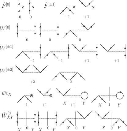
Figure 1: Diagrammatic form of the one- $\hat{F}^{[n]}$ and two-particle $\hat{W}^{[n]}$ (Eq. 7) operators with particle excitation rank number $n$ listed. Also shown are the effective one-electron $\widehat{wc}_{X}$ (Eq. 26) and dimer $W^{[0]}_{XY}$ Brandow-type diagrams (the remaining dimer $W^{[n]}_{XY}$ are expressed in a similar fashion, see Eq. 23 for the algebraic form).

II.2 Effective molecular cluster Hamiltonians

Before proceeding to the derivation of second-order MCPT, it is convenient to define the following monomer specific index domains

$$p,p_{1},r,r_{1},a,i,a_{1},i_{1},\dots\in{\cal H}(X)$$ (19)

and

$$q,q_{1},s,s_{1},b,j,b_{1},j_{1},\dots\in{\cal H}(Y)$$ (20)

where $a,b,\dots$ refer to virtual orbitals and $i,j,\dots$ refer to occupied orbitals while $p,q,\dots$ range over both occupied and virtual orbitals. These index domains will be used to completely define the range of all tensors used hereafter. The monomer Hamiltonian, $\hat{H}_{X}$, is then given in second-quantized form by

$$\hat{H}_{X}= \langle 0|\hat{H}_{X}|0\rangle+\sum_{pp_{1}}f^{p}_{p_{1}}\{\hat{p}^{\dagger}\hat{p}_{1}\}+\frac{1}{4}\sum_{pp_{1}rr_{1}}\bar{v}^{pp_{1}}_{rr_{1}}\{\hat{p}^{\dagger}\hat{p}^{\dagger}_{1}\hat{r}_{1}\hat{r}\}$$ (21)

$$= \langle 0|\hat{H}_{X}|0\rangle+\hat{F}_{X}+\hat{W}_{X}$$ (22)

while the dimer Hamiltonian $\hat{H}_{XY}$ is given by

$$\hat{H}_{XY}= \langle 0|\hat{H}_{XY}|0\rangle+\sum_{pp_{1}}h^{p}_{p_{1}}\{\hat{p}^{\dagger}\hat{p}_{1}\}$$ (23)

$$+\sum_{qq_{1}}h^{q}_{q_{1}}\{\hat{q}^{\dagger}\hat{q}_{1}\}+\sum_{pqrs}\bar{v}^{pq}_{rs}\{\hat{p}^{\dagger}\hat{q}^{\dagger}\hat{s}\hat{r}\}$$ (24)

$$= \langle 0|\hat{H}_{XY}|0\rangle+\widehat{wc}^{[\pm 1]}_{X}+\widehat{wc}^{[\pm 1]}_{Y}+\hat{W}_{XY}.$$ (25)

Here, the monomer and dimer one- ($\hat{F}_{X}$) and two- ($\hat{W}_{X}$ and $\hat{W}_{XY}$) particle operators are defined appropriately in either the monomer or dimer subspace as dictated by the indices. The one-particle operator $\widehat{wc}_{X}$ (see Fig. 1) is defined rybak1991 as

$$\widehat{wc}_{X}=w^{a}_{i}\hat{a}^{\dagger}\hat{i}$$ (26)

where the matrix elements

$$w^{a}_{i}=h^{a}_{i}+2v^{aj}_{ij},$$ (27)

are composed of the one-electron integrals

$$h^{a}_{i}=-\sum_{\mu\nu\in{\cal H}(X)}C_{\mu a}C_{\nu i}\int d{\bf r_{1}}d{\bf r_{2}}\psi^{*}_{\mu}({\bf r_{1}})\sum_{\begin{subarray}{c}Y\neq X\\ \alpha\in Y\end{subarray}}\frac{Z_{\alpha}}{R_{\alpha}-r_{1}}\psi_{\nu}({\bf r_{1}})$$ (28)

which includes the effect of all system nuclei on the wavefunction of $X$, where $C_{\mu p}$ are the monomer Hartree-Fock coefficients and $\psi_{\nu}({\bf r_{1}})$ are gaussian basis functions belonging to monomer $X$. The $v^{aj}_{ij}$ two-electron integrals are evaluated as a special case from

$$(pr|qs)=\sum_{\begin{subarray}{c}\mu\nu\in{\cal H}(X)\\ \lambda\sigma\in{\cal H}(Y)\end{subarray}}C_{\mu p}C_{\nu r}C_{\lambda q}C_{\sigma s}\int d{\bf r_{1}}d{\bf r_{2}}\psi^{*}_{\mu}({\bf r_{1}})\psi_{\nu}({\bf r_{1}})r^{-1}_{12}\psi^{*}_{\lambda}({\bf r_{2}})\psi_{\sigma}({\bf r_{2}})$$ (29)

with $\lambda=\sigma$. It should be noted that the Hartree-Fock orbitals on each monomer are not orthogonalized with other monomers. Using the approximation of Eq. 2 to define our Hartree-Fock vacuum, we can develop our MCPT embedding method.

The monomer and dimer Hamiltonians can still be partitioned in terms of reference and perturbation Hamiltonians

$$\hat{H}_{X}=\hat{H}_{X0}+\hat{V}_{X}$$ (30)

and

$$\hat{H}_{XY}=\hat{H}_{XY0}+\hat{V}_{XY},$$ (31)

where we again use the particle excitation rank partitioning given by (see Fig. 1 for the Brandow-type diagrams for $\hat{H}_{XY0}$)

$$\hat{H}_{X0} =\hat{F}^{[0]}_{X}+\hat{W}^{[0]}_{X},$$ (32)

$$\hat{V}_{X} =\hat{F}^{[\pm 1]}_{X}+\hat{W}^{[\pm 1]}_{X}+\hat{W}^{[\pm 2]}_{X},$$ (33)

$$\hat{H}_{XY0} =\hat{W}^{[0]}_{XY},\text{~{}and}$$ (34)

$$\hat{V}_{XY} =\widehat{wc}^{[\pm 1]}_{X}+\widehat{wc}^{[\pm 1]}_{Y}+\hat{W}^{[\pm 1]}_{XY}+\hat{W}^{[\pm 2]}_{XY}.$$ (35)

Throughout this work, the lower case “$t$” is reserved for singles amplitudes, with upper case “$T$” and script “$\cal T$” reserved for monomer and dimer doubles amplitudes, respectively. Using this notation the system coupled-cluster amplitudes can be expressed as

$$\hat{T}=\sum_{X}\hat{T}_{X}+\sum_{X,Y\neq X}\hat{T}_{XY}$$ (36)

where the cluster operator for monomer $X$,

$$\hat{T}_{X}={\hat{t}}^{(1)}_{X}+{\hat{T}}^{(2)}_{X},$$ (37)

contains the singles and doubles operators defined as

$${\hat{t}}^{(1)}_{X}=\sum_{ai}t^{a}_{i}\hat{a}^{\dagger}\hat{i}$$ (38)

and

$${\hat{T}}^{(2)}_{X}=\frac{1}{4}\sum_{aa_{1}ii_{1}}T^{aa_{1}}_{ii_{1}}\{\hat{a}^{\dagger}\hat{a}_{1}^{\dagger}\hat{i}_{1}\hat{i}\},$$ (39)

respectively, while the cluster operator for the $XY$ dimer only has a doubles contribution (there can be no ${\hat{t}}^{(1)}_{XY}$ in a monomer centered basis) given by

$$\hat{T}_{XY}=\hat{T}^{(2)}_{XY}=\sum_{abij}{\cal T}^{ab}_{ij}\hat{a}^{\dagger}\hat{b}^{\dagger}\hat{j}\hat{i}.$$ (40)

Using Eqs. 36, 37, and 40 it is possible to transform the system Hamiltonian (Eq. 5) into an effective monomer and dimer Hamiltonian as

$${\tilde{H}}_{X}=\left[e^{-\hat{T}+\hat{T}_{X}}\hat{H}e^{\hat{T}-\hat{T}_{X}}\right]_{X}$$ (41)

and

$${\tilde{H}}_{XY}=\left[e^{-\hat{T}+\hat{T}^{(2)}_{XY}}\hat{H}e^{\hat{T}-\hat{T}^{(2)}_{XY}}\right]_{XY}$$ (42)

where the brackets $\left[\dots\right]_{X}$ and $\left[\dots\right]_{XY}$ denote that only terms operating in the monomer ${\cal H}(X)$ and dimer ${\cal H}(X)\otimes{\cal H}(Y)$ Hilbert spaces remain. All terms within the brackets not a member of the appropriate final space to be are internally contracted away. Expanding the Baker-Campbell-Hausdorff (BCH) commutator in Eq. 41 in the same manner as Eqs. 15 and 16 (keeping to the appropriate order in $\hat{V}$) gives

$$\tilde{H}_{X} =\hat{H}_{X}+\widehat{wc}_{X}+\sum_{Y\neq X}\left[\hat{H}_{XY0},\hat{T}_{Y}+\hat{T}_{XY}\right]$$ (43)

$$=\hat{H}_{X0}+\tilde{V}_{X}$$ (44)

with

$$\tilde{V}_{X}=\hat{V}_{X}+\widehat{wc}_{X}+\sum_{Y\neq X}\left[\hat{H}_{XY0},\hat{t}^{(1)}_{Y}+\hat{T}^{(2)}_{XY}\right].$$ (45)

Similarly, the dimer effective Hamiltonian in Eq. 42 can be expanded to give

$$\tilde{H}_{XY}=\hat{H}_{XY0}+\hat{V}_{XY}+\left[\hat{H}_{XY0},\hat{T}^{(2)}_{X}+\hat{T}^{(2)}_{Y}\right].$$ (46)

These effective Hamiltonians have the property that the monomer and dimer Hamiltonians are at this point only members of that specific Hilbert space: $\tilde{H}_{X}\in{\cal H}(X)$ and $\tilde{H}_{XY}\in\{{\cal H}(X)\otimes{\cal H}(Y)={\cal H}(XY)\}$. Contributions from $Y$ in the $\tilde{H}_{X}$ effective Hamiltonian are completely internally contracted away at this point. The monomer and dimer polarization components of the Schrödinger equation for the system can now be written, respectively, as

$$e^{-\hat{T}_{X}}\left(\tilde{H}_{X}-E^{(2)}_{\rm monomer}\right)e^{\hat{T}_{X}}|\phi_{X}\rangle=0$$ (47)

and

$$e^{-\hat{T}_{XY}}\left(\tilde{H}_{XY}-E^{(2)}_{\rm dimer}\right)e^{\hat{T}_{XY}}|\phi_{X}\rangle\otimes|\phi_{Y}\rangle=0.$$ (48)

The corresponding amplitude equations can be obtained straightforwardly from Eqs. 47 and 48 giving

$$\langle\phi_{X}^{g}|\left[\hat{H}_{X0},\hat{T}_{X}\right]+\hat{V}_{X}+\widehat{wc}_{X}+\sum_{Y\neq X}\left[\hat{H}_{XY0},\hat{t}^{(1)}_{Y}+\hat{T}^{(2)}_{XY}\right]|\phi_{X}\rangle=0.$$ (49)

and

$$\langle\phi_{Y}^{g}|\otimes\langle\phi_{X}^{g}|\left[\hat{H}_{XY0},\hat{T}_{XY}\right]+\hat{V}_{XY}+\left[\hat{H}_{XY0},\hat{T}^{(2)}_{X}+\hat{T}^{(2)}_{Y}\right]|\phi_{X}\rangle\otimes|\phi_{Y}\rangle=0.$$ (50)

By transforming to these effective Hamiltonians, we have made clear the electrostatic, induction and dispersion-like monomer and dimer effects from monomer $Y$ into the monomer $X$ Hamiltonian. However, instead of the physically separable bare integral terms rybak1991 these contributions are inseparably included to infinite-order through the coupled-cluster amplitudes by the terms

$$\widehat{wc}_{X}+\sum_{Y\neq X}\left[\hat{H}_{XY0},\hat{t}^{(1)}_{Y}+\hat{T}^{(2)}_{XY}\right].$$ (51)

There are also the corresponding monomer corrections into the dimer potential via

$$\left[\hat{H}_{XY0},\hat{T}^{(2)}_{X}+\hat{T}^{(2)}_{Y}\right].$$ (52)

The inclusion of the induction/dispersion interaction of all other monomers, $Y$, in the amplitude equation of monomer $X$ through Eq. 45 has several important implications. Firstly, at zeroth-order each monomer wavefunction includes the inductive field of the surrounding system. Secondly, while interactions are limited to pairwise terms only, each monomer feeds back into the inductive field of the system iteratively. This means that each monomer includes not just all pairwise interactions but all products of pairwise interactions to infinite-order. To graphically illustrate this point, Fig. 2c contains an illustration of the pairwise communication topology. Here monomers $A$, $B$ and $C$ and monomers in the $D^{\prime}$ and $E^{\prime}$ grouping have all combinations of pairwise interactions at zeroth-order. On the second step of the iterative solution monomer $A$ will now contain information from the entire $D^{\prime}$ and $E^{\prime}$ grouping as well as the $BC$ interaction. Continuing this process iteratively it is evident that, for example, monomer $A$ will contain the information of all possible pairwise interactions. An approximation of immediate concern is the use of a cutoff radius ($R_{\rm cut}$) when deciding what explicit dimer interactions to include in equations 49 and 50. The introduction of such a cut off greatly reduces the computational cost of the amplitude equations, while introducing what would be a small error due to the infinite-order nature of the pairwise contribution.

II.3 Working spin-adapted MCPT(2) equations and program flow

Standard second quantization techniques can be used to obtain the cluster and pairwise additive amplitudes as well as the associated monomer and 2-body polarization energy equations. For the sake of brevity, we forgo a detailed derivation and simply present the final spin-adapted equations using the spin-restricted Hartree-Fock reference as implemented in our program. With the cluster definitions from Eqs. 37-40 and the energy Eqs. 47 and 48 we can write the explicit energy equations. From here on summation over repeated lower and upper indices is implied. The monomer $X$ singles (M1) and doubles (M2) energy contributions are given by

$$E^{(2)}_{\rm M1}(X)=2w^{i}_{a}t^{a}_{i}$$ (53)

and

$$E^{(2)}_{\rm M2}(X)=(2v^{ii_{1}}_{aa_{1}}-v^{i_{1}i}_{aa_{1}})T^{aa_{1}}_{ii_{1}}$$ (54)

for the doubles energy while the $XY$ dimer doubles (D2) energy is defined as

$$E^{(2)}_{\rm D2}(XY)=4v^{ij}_{ab}{\cal T}^{ab}_{ij}.$$ (55)

The monomer doubles energy shift is relative to the isolated monomer $X$ LCCD energy as

$$\delta E^{(2)}_{\rm M2}(X)=E^{(2)}_{\rm M2}(X)-E_{\rm LCCD}(X).$$ (56)

Using Eqs. 37-40 with Eqs. 49 and 50 the monomer singles amplitude equations are

$$\epsilon^{i}_{a}t^{a}_{i}+(2v^{ai_{1}}_{ia_{1}}-v^{ai}_{a_{1}i_{1}})t^{a_{1}}_{i_{1}}+w^{a}_{i}+\sum_{\begin{subarray}{c}Y\neq X_{A}\\ c,k\in{\cal H}(Y)\end{subarray}}\Bigl{(}v^{ak}_{ic}t^{c}_{k}\Bigr{)}=0,$$ (57)

while the monomer and dimer doubles amplitudes are defined as

$$\epsilon^{ii_{1}}_{aa_{1}}T^{aa_{1}}_{ii_{1}}+v^{aa_{1}}_{ii_{1}}+v^{aa_{1}}_{a_{2}a_{3}}T^{a_{2}a_{3}}_{ii_{1}}+v_{ii_{1}}^{i_{2}i_{3}}T^{aa_{1}}_{i_{2}i_{3}}+(v^{ai_{2}}_{ia_{2}}-v^{ai_{2}}_{a_{2}i})T^{a_{2}a_{1}}_{i_{2}i_{1}}+(v^{a_{1}i_{2}}_{i_{1}a_{2}}-v^{a_{1}i_{2}}_{a_{2}i_{1}})T^{a_{2}a}_{i_{2}i}\\ +v^{i_{2}a}_{a_{2}i}(T^{a_{2}a_{1}}_{i_{2}i_{1}}-T^{a_{2}a_{1}}_{i_{1}i_{2}})+v^{i_{2}a_{1}}_{a_{2}i_{1}}(T^{a_{2}a}_{i_{2}i}-T^{a_{2}a}_{ii_{2}})-v^{a_{1}i_{2}}_{a_{2}i}T^{aa_{2}}_{i_{2}i_{1}}-v^{ai_{2}}_{a_{2}i_{1}}T^{a_{1}a_{2}}_{i_{2}i}\\ +\sum_{\begin{subarray}{c}Y\neq X_{A}\\ c,k\in{\cal H}(Y)\end{subarray}}\left(v^{a_{1}k}_{i_{1}c}{\cal T}^{ac}_{ik}+v^{ak}_{ic}{\cal T}^{a_{1}c}_{i_{1}k}\right)=0$$ (58)

and

$$\epsilon^{ij}_{ab}{\cal T}^{ab}_{ij}+v^{ab}_{ij}+v^{ab}_{a_{1}b_{1}}{\cal T}^{a_{1}b_{1}}_{ij}+v^{i_{1}j_{1}}_{ij}{\cal T}^{ab}_{i_{1}j_{1}}-v^{bi_{1}}_{b_{1}i}{\cal T}^{ab_{1}}_{i_{1}j}-v^{aj_{1}}_{a_{1}j}{\cal T}^{a_{1}b}_{ij_{1}}+(2v^{i_{1}a}_{a_{1}i}-v^{ai_{1}}_{a_{1}i}){\cal T}^{a_{1}b}_{i_{1}j}\\ +(2v^{j_{1}b}_{b_{1}j}-v^{bj_{1}}_{b_{1}j}){\cal T}^{ab_{1}}_{ij_{1}}+\left(v^{i_{1}b}_{a_{1}j}(2{T}^{aa_{1}}_{ii_{1}}-{T}^{aa_{1}}_{i_{1}i})+v^{j_{1}a}_{b_{1}i}(2T^{bb_{1}}_{jj_{1}}-T^{bb_{1}}_{j_{1}j})\right)=0$$ (59)

respectively. For clarity, the summation over the $c,k$ indices is explicitly written in Eqs. 57 and 58. The energy tensor used above is defined as

$$\epsilon^{ij\cdots}_{ab\cdots}=\epsilon_{i}+\epsilon_{j}+\cdots-\epsilon_{a}-\epsilon_{b}-\cdots$$ (60)

where $\epsilon_{p}$ is the $p$’th Hartree-Fock orbital energy, the energy denominator is then

$$D^{ij\cdots}_{ab\cdots}=1/\epsilon^{ij\cdots}_{ab\cdots}.$$ (61)

The energy equations 53-55, and amplitude equations 57-59 define the second-order MCPT embedding method. With all the pertinent equations derived we are able now to summarize the overall algorithm. Note that in the following $X$ and $Y$ remain dummy indices over monomers, $N$ is the number of monomers and $R_{\rm cut}$ is the distance cutoff value.

1. For each monomer in the system a Hartree-Fock calculation is performed in the monomer centered basis set neglecting all environment contributions. The resulting monomer specific molecular orbitals (MO) are stored.

2. The two-electron integrals are computed and transformed into the monomer, and direct product MO basis (see Eq. 29). If a cutoff radius is to be used, only dimers that satisfy the distance criteria are included.

3. The one-electron $\widehat{wc}$ operator is formed.

4. Using $w^{a}_{i}$ as an initial guess to $t^{a}_{i}$ the singles amplitudes are iterated over until convergence as:

   for all CC iterations do

        for $1\leq X\leq N$ do

            for all $Y$ satisfying $R_{\rm cut}$ do

                 Construct $\sum v^{ak}_{ic}t^{c}_{k}$.

            end for

            Construct $t^{a}_{i}$ (Eq. 57).

            Compute $E^{(2)}_{\rm M1}$ (Eq. 53).

            if $E^{(2)}_{\rm M1}$ is converged then

                 Exit

            end if

        end for

   end for

5. Compute LCCD energies for each monomer in the monomer centered basis set again neglecting all environment contributions.

6. Using $v^{aa_{1}}_{ii_{1}}$ and $v^{ab}_{ij}$ as an initial guess, the $T^{aa_{1}}_{ii_{1}}$ and ${\cal T}^{ab}_{ij}$ doubles amplitudes are iterated over in a macro and micro iteration fashion until converged as illustrated:

   for all CC macro iterations do

        for $1\leq X\leq N$ do

            for all CC micro iterations do

                 for all $Y$ satisfying $R_{\rm cut}$ do

                     Construct $v^{a_{1}k}_{i_{1}c}{\cal T}^{ac}_{ik}+v^{ak}_{ic}{\cal T}^{a_{1}c}_{i_{1}k}$

                 end for

                 Construct $T^{aa_{1}}_{ii_{1}}$ (Eq. 58).

                 Compute $E^{(2)}_{\rm M2}$ (Eq. 54).

                 if $E^{(2)}_{\rm M2}$ is converged then

                     Exit

                 end if

            end for

        end for

        for $1\leq X\leq N$, $1\leq Y\leq N$ do

            if $X\neq Y$ and $R_{\rm cut}$ is satisfied then

                 for all CC micro iterations do

                     Construct ${\cal T}^{ab}_{ij}$ (Eq. 59).

                     Compute $E^{(2)}_{\rm M2}$ (Eq. 55).

                     if $E^{(2)}_{\rm D2}$ is converged then

                          Exit

                     end if

                 end for

            end if

        end for

   end for

The practical computational benefit of using the MCPT(2) method can be seen by examining the most intensive part of the calculation (Eqs. 58 and 59) described in bullet (6) above. Using $M$ and $\tilde{M}$ to denote the total number of monomer- and dimer-doubles (first and second sub loops respectively) micro iterations the effective computational scaling of the entire calculation is $O\left((M+\tilde{M})\times N\tilde{N}\times o^{2}v^{4}\right)$, where $N$ denotes the number of monomers in the system, $\tilde{N}$ is the largest number of monomers contained within the cutoff radius $R_{\rm cut}$ and the number of occupied and virtual orbitals corresponds to the largest included monomer. This is contrasted by the corresponding LCCD scaling of $O(M\times N^{6}\times o^{2}v^{4})$ which will always be more costly so long as $\tilde{M}\tilde{N}<N^{5}$. It is our experience in practice for $\tilde{M}\sim 15$ so that only for two monomers is LCCD less computationally intensive.

As an additional note, in the computation of first-order properties it is convenient to work with the one-particle density matrix (1DM). This monomer 1DM is defined in the AO basis as

$$\rho_{\mu\nu}=\sum_{ij}C_{\mu i}C_{\nu j}-\sum_{pq}C_{\mu p}\rho_{pq}C_{\nu q}$$ (62)

where $\rho_{pq}$ is the response density computed from the monomer cluster amplitudes $\hat{T}_{X}$ and the indices $p,q$ range over both occupied and virtual orbitals. The contribution from exchange between monomers $X$ and $Y$ can be obtained at the Hartree-Fock level by examining

$$\langle\phi_{X}|\hat{O}\hat{P}|\phi_{X}\rangle$$ (63)

where $\cal O$ is the one-particle property operator, and we define then the Hartree-Fock exchange density as

$$\bar{\rho}_{\mu\bar{\nu}}=\sum_{\mu^{\prime}\bar{\nu}^{\prime}}\sum_{ij}C_{\mu i}C_{\mu^{\prime}j}S^{\bar{\nu}^{\prime}}_{\mu^{\prime}}\sum_{\bar{k}\bar{\ell}}C_{\bar{\nu}^{\prime}\bar{k}}C_{\bar{\nu}\bar{\ell}}.$$ (64)

for all $\mu,\mu^{\prime},i,j\in{\cal H}(X)$ and $\bar{\nu},\bar{\nu}^{\prime},\bar{k},\bar{\ell}\in{\cal H}(Y)$, where $S^{\bar{\nu}^{\prime}}_{\mu^{\prime}}$ is the overlap matrix between monomers rybak1991 . A first-order property can be evaluated through the expectation value of the wavefunction as

$$\langle\hat{\cal O}\rangle=Tr({\bf{\cal O}\rho})+Tr({\bf{\cal O\bar{\rho}}}),$$ (65)

where the first term is the monomer only value and the second is the non-local dimer contribution.

III Electronic Structure Calculations

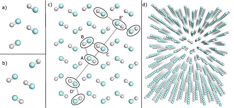
Figure 2: HF molecules in a crystal; a$)$ Polar unit cell, b$)$ Non-Polar unit cell. c$)$ Mono-layer of crystal HF in the non-polar ($8\times 8\times 8$) polymorph. Also shown diagrammatically is an example of the pairwise monomer-monomer communication topology. d$)$ Schematic of the largest HF crystal cube (show is the non-polar polymorph) considered in this paper. With 1,000 explicit HF molecules in the aug-cc-pCVDZ basis set there is 32,000 basis set functions in total.

Electronic structure calculations were performed on the University of Florida HiPerGator high performance cluster and the Cray (XE6) Garnet based at the ERDC DoD Supercomputer Resource Center. The all ab initio results were obtained using the new Aces4 massively parallel ab initio quantum chemistry package based on the new implementation of the Super Instruction Architecture lotrich2010 (SIA) program.

The current implementation of MCPT does not include the ability to freeze the core electrons of the monomers. To guarantee a balanced treatment of the electronic correlation, we use the core-valence version of the Dunning correlation consistent basis sets woon1995 (cc-pCVnZ) on all heavy atoms with the corresponding standard basis dunning1989 (cc-pVnZ) on hydrogen. To aid in the basis set convergence of computed energies and dipole moments halkier1999 , diffuse functions kendall1992 (aug-) were added to each atom’s basis set. It is established in this work and elsewhere that dipole moments halkier1999 and HF molecular harmonic frequencies are described reasonably with just the aug-cc-pCVDZ basis set.

Immensely instrumental in the practical implementation and use of the MCPT methodology is the recently reimplemented SIA. The extremely large arrays required are automatically partitioned and distributed, and are allocated only as needed. They can be very conveniently manipulated from SIAL lotrich2010 , the domain specific programming language used to script calculations. This means that by expanding in the direct product space (Eq. 2) we have introduced a block sparsity into the system which is fully exploited by the dynamic memory management system.

IV Numerical Results and Discussion

IV.1 Hydrogen fluoride crystal

Figure 3: Convergence of the polar unit cell monomer energy shifts as a function of the distance cutoff $R_{\rm cut}$. The difference between the singles energy shift at $10.5$ and $12.0$ Å is $4$ cm^-1, and for the doubles energy shift the difference is $1$ cm^-1. The cutoff values were chosen to correspond to the separation between HF layers.

As previously discussed, the tremendous computational scaling reduction obtained by working within an iterative pairwise interaction framework means that scaling quantum systems to the bulk limit is accessible. In this section, we illustrate just how flexible this framework is by examining the HF molecular crystal from a starting seed of eight molecules up through the bulk limit using a thousand molecules. The double $\zeta$ quality basis set (aug-cc-pCVDZ) was used here for all calculations, which provides qualitatively accurate energetics (except for very small energy differences on the order of a few kcal/mol) and well converged dipole moments. The total HF crystal structure was generated by building up HF ”1-D” polymers into a regular cube. Spacings between HF molecules within and between the polymer chains was chosen as to replicate the experimental lattice constants atoji1954 . The H-F bond length was fixed at 0.92 Å  so as to agree with this the same experiment. The two basic unit cells, denoted polar and non-polar here, are illustrated in Fig. 2a-b. Also shown in Fig. 2c-d is the HF crystal cube mono-layer and the final 3-D structure. Bulk limit scaling calculations were performed for both the polar (Fig. 2a) and non-polar (Fig. 2b) polymorphs. The size of the HF cube for both polymorphs was increased from $2\times 2\times 2$ to $10\times 10\times 10$, systematically. The largest structure considered (the $10\times 10\times 10$ lattice) has $\sim 32,000$ basis set functions and $10,000$ electrons. In all crystal calculations a dimer radius cutoff of $12$ Å  was used. With these lattice parameters the size of the $10\times 10\times 10$ crystal is $20\times 20\times 30$ Å. Choosing a $12$ Å  cutoff results in a maximum of $\tilde{N}\sim 350$ (with an average of $\tilde{N}\sim 210$) monomers included within the threshold. Numerical experimentation showed that a much smaller (next nearest neighbors) cutoff is sufficient to converge the MCPT doubles amplitudes to within 0.1 kcal/mol. However the electrostatic contributions are not converged to the same degree until at least the $10.5$ Å  cutoff distance. This is illustrated for the polar lattice in Fig. 3.

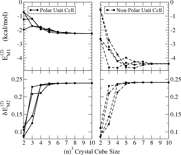
Figure 4: Monomer energy shifts for the four member HF molecules of the central unit cell for increasing crystal size.

In Fig. 4, we show the shift in energy coming from the $E^{(2)}_{\rm M1}$ and $\delta E^{(2)}_{\rm M2}$ contribution for the four HF molecules forming the central unit cell. Because the crystal is explicitly computed with no periodic boundary conditions, each internal HF molecule experiences a different environment (including any surface polarization effects). To obtain true bulk limit quantities it is necessary to increase the crystal size until interactions between the central unit cells become uniform. We use as a metric for convergence the energy shift of the four member HF molecules of the central unit cell. The energy shifts perform well in this role as these quantities are very sensitive to the surrounding environment. Small deviations due to the addition of more HF molecules to the crystal (the invariance to adding more molecules to the system being the definition of bulk limit) become evident on the milli- and microHartree scale, well within the numerical convergence of our calculations.

The initial $2\times 2\times 2$ cube is a largely artificial construct in this bulk limit scaling analysis. It is included as it illustrates the expected monomer energy shift symmetry between adjacent HF chains. As is clear for the following small cluster sizes (3-4 per side), the energy shift varies greatly within the central unit cell. This is expected; surface effects still drastically affect the central system. Scaling the cluster size past 5 molecules per side demonstrates that the $\delta E^{(2)}_{\rm M2}$ energy shift is essentially converged, with the $E^{(2)}_{\rm M1}$ contribution nearly so. The accelerated convergence of the $\delta E^{(2)}_{\rm M2}$ energy contributions can be understood from the fact that this term is dominated by dispersion- and induction-type interactions, which drop off as $1/R^{6}$ with the intermolecular distance. Thus contributions from anything beyond nearest neighbors are necessarily going to be small. This is contrasted by the $E^{(2)}_{\rm M1}$ contribution which is dominated by long-range dipole type interactions that do not fully converge until at least 7 molecules per side. We find the $E^{(2)}_{\rm M1}$ energy shift converges for both the $10\times 10\times 10$ polar and non-polar cube with an energy variance within the unit cell of less than a micro-Hartree.

With the perturbed HF molecular wavefunction on hand, it is straightforward to compute the first-order response properties. In this work, we examine the dipole moment, via using the first term of Eq. 65. Computing the dipole moment for each HF molecule in the lattice produces an imperceptible change from the gas phase dipole moment of 1.90 Debye. This result is expected as the idea of a local monomer density within a polar crystal is merely a theoretical construct. The average HF lattice site dipole moment per unit cell can still be assigned by computing the non-local exchange contribution to the electronic density and then assigning a portion of the density to a specific HF molecule domain. The non-local density is computed using Eq. 64, which uses the SCF exchange density between nearby molecule pairs. Taking all these effects into account, the computed average dipole moments within the central unit cell are found to be 2.51 and 2.49 Debye for the polar and non-polar structures respectively. These are in excellent agreement with the published values sode2010 of 2.51 and 2.47 Debye using MP2/aug-cc-pVDZ.

Any quantity directly dependent on the monomer wavefunction (and energy), including environmental effects, is of course obtainable within the MCPT framework. Monomer structures, conformational orderings, and vibrational spectra are some examples that could be examined. We can further illustrate the utility of the MCPT method by computing the harmonic vibrational (stretch) modes of the non-polar polymorph of the HF lattice. This kind of property is readily computed numerically by displacements of the nuclear coordinates and thus requires no new methodological advancement. With knowledge of the orthorhombic $D_{2h}$ stretch modes hornig1955 , we can obtain the requisite single point calculations by performing symmetric displacements about the F-H equilibrium along the four specific stretch modes ($\rm S(A_{g}),~{}S(B_{3u}),~{}S(B_{2u})\text{~{}and~{}}S(B_{1g})$) within the unit cell. A 5-point grid for the finite-difference second derivative with a displacement step size of $0.01$ Å was used with the approximation that the fluorine atoms remain fixed. The single point energies used are constructed additively from Eqs. 53 and 54 by

$$E^{(2)}_{\rm MCPT}=\sum_{X}\left(E_{\rm SCF}(X)+E^{(2)}_{M1}(X)+E^{(2)}_{M2}(X)\right)$$ (66)

where the sum is over the four HF molecules in the central unit cell. Having identified that the monomer shift of the central unit cell in the $10\times 10\times 10$ lattice has converged to the bulk limit, we use the same crystal size and lattice constants for the frequency calculation for consistency. The resulting stretch frequencies are given in Table 1 as well as a reference LCCD harmonic frequency calculation for the gas phase HF molecule. We recover most of the observed frequency shift relative to the gas phase, with our predicted ordering and relative energies in agreement with experiment kittelberger1967 ; anderson1980 ; pinnick1989 . As also observed in prior periodic wavefunction results sode2012 , the further lowering of the $\rm S(A_{g})$ and $\rm S(B_{3u})$ modes relative to the $\rm S(B_{2u})$ and $\rm S(B_{1g})$ modes is not achieved. This comparison with the values from Sode et al. is relevant as theirs are the only other computational value in the literature. Further improvement to the absolute placement of the predicted spectra can be expected through optimization of the lattice parameters, larger basis sets, and other improved approximations which we leave to future work.

Isolated HF molecule	$\omega_{e}$
LCCD/aug-cc-pCVDZ	4121
CCSD/aug-cc-pCVDZ	4130
Exp leroy1998	4138

	$\rm S(A_{g})$	$\rm S(B_{3u})$	$\rm S(B_{2u})$	$\rm S(B_{1g})$
MCPT(2)/aug-cc-pCVDZ	3696	3724	3758	3770
Infrared kittelberger1967		3067	3406
Raman anderson1980	3045			3386
Raman pinnick1989	3027			3376
Periodic wavefunction sode2012	3555	3458	3584	3570

Table 1: Computed harmonic vibrational frequency for the gas phase HF molecule and the four stretch modes of the non-polar polymorph HF crystal (10$\times$10$\times$10 lattice). Units are in cm^-1.

V Conclusions

In this work we have focussed on two specific goals: the formulation of a new explicit molecular cluster based perturbation theory, and a program implementation of said perturbation theory that is capable of scaling to the bulk limit. Our first goal has led us to develop the linearly scaling second-order molecular cluster perturbation theory. MCPT(2) contains infinite-order contributions to the monomer electronic correlation energy and is infinite-order in the pairwise dimer interaction (infinite-order by including all pairwise, and all possible products of pairs). We started with coupled-cluster perturbation theory with the particle excitation rank Hamiltonian partitioning, as used by us before bartlett2010 ; byrd2014-b ,with the reference wavefunction taken to be a product of monomer Hartree-Fock wavefunctions. Limiting the cluster expansion to only monomer and dimer interactions, a similarity transformation is performed to obtain effective Hamiltonians that only operate on the monomer, $\tilde{H}_{X}\in{\cal H}(X)$, and dimer, $\tilde{H}_{XY}\in{\cal H}(XY)$, Hilbert spaces. These effective Hamiltonians allow us to directly use the CCPT framework, and help elucidate the pairing between cluster operators of the surrounding cluster on that of a given monomer or dimer.

By working with at most explicit pairwise interactions within a cutoff, the prohibitive $O(N^{6}o^{2}v^{4})$ computational scaling of a full CCSD explicit calculation is reduced to $O(\tilde{N}No^{2}v^{4})$ ($\tilde{N}$ is the maximum number of monomers possible within the given cutoff radius). For the benchmark crystal studied here (the $10\times 10\times 10$ HF square crystal), the computation savings of going from the full CCSD to the MCPT(2) framework is a factor of $10^{6}$, with an additional factor of $3$ ($\tilde{N}\sim 350$) savings through the inclusion of a cutoff. Independent of the methodological choices that reduce computational cost, the use of innovations in the computer science of the SIA model Despite the reduction due to pairwise interactions, the necessary arrays remain large. The automatic partitioning and inherent block sparsity capability provided by SIA has allowed us to perform our largest HF crystal calculations on just 256 processors within a standard $12$ hour queue length.

By using the MCPT(2) framework, we obtain not just monomer energies that include interactions of the surrounding system to infinite-order, but also the specific monomer wavefunction as well. This opens up future investigations not just in monomer energetic such as vibrational energy shifts or monomer conformer orderings, but also direct computation of first and second-order properties of the monomers.

VI Acknowledgements

J.N.B., V.F.L. and R.J.B. acknowledge funding support from the United States Air Force Office of Scientific Research grant FA 9550-11-1-0065 N.J. and B.A.S. were supported by the National Science Foundation Grant OCI-0725070 and the Office of Science of the U.S. Department of Energy under grant DE-SC0002565. Additional acknowledge must be given to the United States Army Research Office DURIP grant W911-12-1-0365 which funded access to the University of Florida Research Computing HiPerGator high performance cluster and provided computer time at the ERDC DoD Supercomputer Resource Center.

References

- (1) N. Flocke and R.J. Bartlett, J. Chem. Phys. 121, 10935 (2004).
- (2) J. Tomasi, B. Mennucci and R. Cammi, Chem. Rev. 105, 2999 (2005).
- (3) M. Gordon, L. Slipchenko, H. Li and J. Jensen, Annu. Rep. Comput. Chem. 3, 177 (2007).
- (4) D.G. Fedorov, T. Nagata and K. Kitaura, Phys. Chem. Chem. Phys. 14, 7562 (2012).
- (5) A. Klamt, WIREs Comput. Mol. Sci. 1, 699 (2011).
- (6) T. Vreven and K. Morokuma, in Annual Reports in Computational Chemistry, edited by D. C. Spellmeyer, Vol. 2, Chap. 3 (Elsevier, Amsterdam, 2006), pp. 35–51.
- (7) R. Podeszwa, B. Rice and K. Szalewicz, Phys. Rev. Lett. 101 (11), 115503 (2008).
- (8) N.J. Mayhall and K. Raghavachari, J. Chem. Theory Comput. 7, 1336 (2011).
- (9) G. Knizia and G. Chan, Phys. Rev. Lett. 109, 186404 (2012).
- (10) M.S. Gordon, D.G. Fedorov, S.R. Pruitt and L.V. Slipchenko, Chem. Rev. 112, 632 (2012).
- (11) A.D. Buckingham, Adv. Chem. Phys. 12, 107 (1967).
- (12) S. Rybak, B. Jeziorski and K. Szalewicz, J. Chem. Phys. 95, 6576 (1991).
- (13) B. Jeziorski, R. Moszynski and K. Szalewicz, Chem. Rev. 94, 1887 (1994).
- (14) G. Chalasinski, B. Jeziorski and K. Szalewicz, Int. J. Quant. Chem 11 (2), 247 (1977).
- (15) V.F. Lotrich and K. Szalewicz, J. Chem. Phys. 106, 9688 (1997).
- (16) M.T. Cvitaš, P. Soldán, J.M. Hutson, P. Honvault and J.M. Launay, J. Chem. Phys. 127, 074302 (2007).
- (17) R. Bartlett and M. Musiał, Rev. Mod. Phys. 79, 291 (2007).
- (18) R. Cammi, J. Chem. Phys 131, 164104 (2009).
- (19) P.J. Bygrave, N.L. Allan and F.R. Manby, J. Chem. Phys. 137, 164102 (2012).
- (20) N.H. List, S. Coriani, J. Kongsted and O. Christiansen, J. Chem. Phys. 141, 244107 (2014).
- (21) R.J. Bartlett, M. Musial, V.F. Lotrich and T. Kus, in Recent Progress in Coupled-Cluster Methods, edited by P. Carsky, J. Paldus and J. Pittner, Vol. 11, Chap. 1 (Springer, Dordrecht, 2010), pp. 1–34.
- (22) G.D. Purvis III and R.J. Bartlett, J. Chem. Phys. 76, 1910 (1982).
- (23) I. Grabowski, V. Lotrich and R.J. Bartlett, J. Chem. Phys. 127 (2007).
- (24) M. Atoji and W. Lipscomb, Acta Cryst 7, 173 (1954).
- (25) M.W. Johnson, E. Sandor and E. Arzi, Acta Crystallogr. Sect. B-Struct. Sci. 31, 1998 (1975).
- (26) P. Otto and E.O. Steinborn, Solid State Commun. 58, 281–284 (1986).
- (27) I. Panas, Int. J. Quantum Chem. 46, 109 (1993).
- (28) S. Berski and Z. Latajka, J. Mol. Struct. 450, 259–263 (1998).
- (29) C. Buth and B. Paulus, Chem. Phys. Lett. 398, 44–49 (2004).
- (30) C. Buth and B. Paulus, Phys. Rev. B 74, 045122 (2006).
- (31) O. Sode and S. Hirata, J. Phys. Chem. A 114, 8873 (2010).
- (32) J.S. Kittelberger and D.F.J. Hornig, Chem. Phys. 46, 3099 (1967).
- (33) A. Anderson, B. Torrie and W. Tse, Chem. Phys. Lett. 70, 300 (1980).
- (34) D. Pinnick, A. Katz and R. Hanson, Phys. Rev. B: Condens. Matter Mater. Phys. 39, 8677 (1989).
- (35) O. Sode, M. Keçeli, S. Hirata and K. Yagi, Int. J. Quantum Chem. 109, 1928–1939 (2009).
- (36) O. Sode and S. Hirata, Phys. Chem. Chem. Phys. 14, 7765 (2012).
- (37) I. Shavitt and R.J. Bartlett (Cambridge, New York, 2009).
- (38) J.N. Byrd, V.F. Lotrich and R.J. Bartlett, J. Chem. Phys. 140, 234108 (2014).
- (39) V.F. Lotrich, J.M. Ponton, A.S. Perera, E. Deumens, R.J. Bartlett and B.A. Sanders, Mol. Phys. 108, 3323 (2010).
- (40) D.E. Woon and T.H. Dunning Jr. , J. Chem. Phys. 103, 4572 (1995).
- (41) T. Dunning Jr, J. Chem. Phys. 90, 1007 (1989).
- (42) A. Halkier, W. Klopper, T. Helgaker and P. Jørgensen, J. Chem. Phys. 111, 4424 (1999).
- (43) R. Kendall, T. Dunning Jr and R. Harrison, J. Chem. Phys. 96, 6796 (1992).
- (44) D.F. Hornig and W.E. Osberg, J. Chem. Phys. 23, 662 (1955).
- (45) R.J. Le Roy, J. Mol. Spec. 194, 189–196 (1999).