Relativistic quantum pseudo-telepathy

Abstract

We analyze the impact of the Unruh effect on quantum Magic Square game. We find the values of acceleration parameter for which quantum strategy yields higher players‘ winning probability than classical strategy.

PACS: 03.67.Ac, 03.67.-a, 03.65.Aa, 03.65.Ud, 02.50.Le
Keywords: quantum games, quantum psuedo-telepathy, Unruh effect

1 Introduction

Quantum game theory is an interdisciplinary field that combines game theory and quantum information. It lies at the crossroads of physics, quantum information processing, computer and natural sciences. Various quantizations of games were presented by different authors [1, 2, 3].

Quantum pseudo-telepathy games [4] form a subclass of quantum games. A game belongs to the pseudo-telepathy class providing that there are no winning strategies for classical players, but a winning strategy can be found if the players share a sufficient amount of entanglement. In these games quantum players can accomplish tasks that are unfeasible for their classical counterparts.

Given a pseudo-telepathy game, one can implement a quantum winning strategy for this game [4]. In an ideal case, the experiment should involve a significant number of rounds of the game. The experiment should be continued until either the players lose a single round or the players win such a great number of rounds, that it would be nearly impossible if they were using a classical strategy. Unfortunately ideal noiseless setup of a quantum game is impossible to be achieved.

The motivation to study the Magic Square game and pseudo-telepathy games in general is that their physical implementation could provide convincing, even to a layperson, demonstration that the physical world is not local realistic. By local we mean that no action performed at some location X can have an effect on some remote location Y in a time shorter then that required by light to travel from X to Y. Realistic means that a measurement can only reveal elements of reality that are already present in the system [4].

It has been shown [5] that noise in a quantum channel can decrease the probability of winning the Magic Square game even below the classical threshold, although the players can counteract this effect for lower noise [6].

2 Magic Square game

The magic square is a $3\times 3$ matrix filled with numbers 0 or 1 so that the sum of entries in each row is even and the sum of entries in each column is odd. Although such a matrix cannot exist (see Fig. 1) one can consider the following game.

1	1	0
1	0	1
1	0	?

Figure 1: An illustrative filling of the magic square with numbers 0 and 1. The question mark shows that it is not possible to put a number in the last field and satisfy both conditions of the game.

The game setup is as follows. There are two players: Alice and Bob. Alice is given a row, Bob is given a column. Alice has to give the entries for a row and Bob has to give the entries for a column so that the parity conditions are met. Winning condition is that the players‘ entries at the intersection must agree. Alice and Bob can prepare a strategy but they are not allowed to communicate during the game.

There exists a (classical) strategy that guarantees the winning probability of $\frac{8}{9}$. If the parties are allowed to share a quantum state they can achieve probability of success equal to one [4].

In the quantum version of this game [7, 8] Alice and Bob are allowed to share an entangled quantum state. The winning strategy is following. Alice and Bob share entangled state

$$|\psi\rangle=\frac{1}{2}\left(|0011\rangle+|1100\rangle-|0110\rangle-|1001\rangle\right)$$ (1)

and apply local unitary operators $A_{i}\otimes B_{j}$, where

$A_{1}$ =	$\frac{1}{\sqrt{2}}\left(\begin{smallmatrix}i&0&0&1\\ 0&-i&1&0\\ 0&i&1&0\\ 1&0&0&i\end{smallmatrix}\right),$	$A_{2}$ =	$\frac{1}{2}\left(\begin{smallmatrix}i&1&1&i\\ -i&1&-1&i\\ i&1&-1&-i\\ -i&1&1&-i\end{smallmatrix}\right),$
$A_{3}$ =	$\frac{1}{2}\left(\begin{smallmatrix}-1&-1&-1&1\\ 1&1&-1&1\\ 1&-1&1&1\\ 1&-1&-1&-1\end{smallmatrix}\right),$	$B_{1}$ =	$\frac{1}{2}\left(\begin{smallmatrix}i&-i&1&1\\ -i&-i&1&-1\\ 1&1&-i&i\\ -i&i&1&1\end{smallmatrix}\right),$
$B_{2}$ =	$\frac{1}{2}\left(\begin{smallmatrix}-1&i&1&i\\ 1&i&1&-i\\ 1&-i&1&i\\ -1&-i&1&-i\end{smallmatrix}\right),$	$B_{3}$ =	$\frac{1}{\sqrt{2}}\left(\begin{smallmatrix}1&0&0&1\\ -1&0&0&1\\ 0&1&1&0\\ 0&1&-1&0\end{smallmatrix}\right).$

Indices $i$ and $j$ label rows and columns of the magic square. Therefore the state of this scheme before measurement is

$$\rho_{f}=(A_{i}\otimes B_{j})\,|\psi\rangle\langle\psi|\,(A_{i}^{\dagger}\otimes B_{j}^{\dagger}).$$ (2)

The final step of the game consists of the measurement in the computational basis.

We are interested in the mean probability of Alice and Bob winning the game. This probability is given by

$$p=\frac{1}{9}\sum\limits_{i,j=1}^{3}\sum_{\xi\in\mathcal{S}_{ij}}\mathrm{Tr}{\rho_{f}}{|\xi\rangle\langle\xi|},$$ (3)

where $\mathcal{S}_{ij}$ is the set of right answers for the column and row $ij$ (Tab. 1). In the case of no acceleration we get $p=1$.

	${0}$	${1}$	${2}$	${3}$	${4}$	${5}$	${6}$	${7}$	${8}$	${9}$	${10}$	${11}$	${12}$	${13}$	${14}$	${15}$
$\mathcal{S}_{11}$	+	+	-	-	+	+	-	-	-	-	+	+	-	-	+	+
$\mathcal{S}_{12}$	+	+	-	-	-	-	+	+	+	+	-	-	-	-	+	+
$\mathcal{S}_{13}$	+	+	-	-	-	-	+	+	-	-	+	+	+	+	-	-
$\mathcal{S}_{21}$	+	-	+	-	+	-	+	-	-	+	-	+	-	+	-	+
$\mathcal{S}_{22}$	+	-	+	-	-	+	-	+	+	-	+	-	-	+	-	+
$\mathcal{S}_{23}$	+	-	+	-	-	+	-	+	-	+	-	+	+	-	+	-
$\mathcal{S}_{31}$	-	+	+	-	-	+	+	-	+	-	-	+	+	-	-	+
$\mathcal{S}_{32}$	-	+	+	-	+	-	-	+	-	+	+	-	+	-	-	+
$\mathcal{S}_{33}$	-	+	+	-	+	-	-	+	+	-	-	+	-	+	+	-

Table 1: Sets $\mathcal{S}_{ij}$ — plus sign (+) indicates that the given element belongs to the set, minus (-) sign indicates that the element does not belong to the set.

3 Magic square game in non-inertial reference frames

In order to derive expressions for the Magic Square game in a non-inertial reference frame, let us consider the initial state of the game as an entangled state of four fermionic qubits of mode frequencies $\omega_{\mathrm{A}}$ and $\omega_{\mathrm{B}}$ in a flat Minkowski space-time:

$$|\psi\rangle=\frac{1}{2}\left(|0_{\omega_{\mathrm{A}}}\rangle|1_{\omega_{\mathrm{B}}}\rangle-|1_{\omega_{\mathrm{A}}}\rangle|0_{\omega_{\mathrm{B}}}\rangle\right)\otimes\left(|0_{\omega_{\mathrm{A}}}\rangle|1_{\omega_{\mathrm{B}}}\rangle-|1_{\omega_{\mathrm{A}}}\rangle|0_{\omega_{\mathrm{B}}}\rangle\right),$$ (4)

where kets $|0_{\omega_{\mathrm{x}}}\rangle$ and $|1_{\omega_{\mathrm{x}}}\rangle$ ($\mathrm{x}\in\{\mathrm{A},\mathrm{B}\}$) represent the vacuum and excited states from the perspective of an inertial observer. The state in Eq. (4) is equivalent to the one defined in Eq. (1) up to a swap operation.

In order to describe accelerated observers, we use Rindler coordinates, which define two casually disconnected regions ($I,II$), i.e. a uniformly accelerated observer in region $I$ has no access to information in region $II$ and vice versa [9]. In order to simplify our scheme, we consider a single mode in the Rindler region $I$. This approach is justified if the observers‘ detectors are highly monochromatic and detect the frequency $\omega_{\mathrm{A}}\approx\omega_{\mathrm{B}}=\omega$. Hereafter, due to this approximation we will omit the subscript of $\omega$.

In an accelerated reference frame, the vacuum state becomes a two mode squeezed state given by [9, 10, 11, 12]

$$|0\rangle=\cos(r)|0\rangle_{I}|0\rangle_{II}+\sin(r)|1\rangle_{I}|1\rangle_{II},$$ (5)

and the excited state becomes

$$|1\rangle=|1\rangle_{I}|0\rangle_{II},$$ (6)

where $I$ and $II$ represents mode in the two Rindler regions. The parameter $r$ is a dimensionless acceleration given by:

$$r=\sqrt{\exp\left(\frac{-2\pi\omega c}{a}\right)+1},$$ (7)

where $a$ is Bob‘s acceleration. The value $r=0$ corresponds to no acceleration and the value $r=\frac{\pi}{4}$ corresponds to infinite acceleration.

Eq. (5) shows that an observer in an non-inertial reference frame, moving with a constant acceleration, sees a thermal state instead of a vacuum state, i.e. observers a black body radiation. This phenomenon is called the Unruh effect [13, 14]

In the case of stationary Alice and accelerating Bob, using the Rindler coordinates we obtain obtain the following initial state

$$|\psi\rangle=|\psi_{(1)}\rangle\otimes|\psi_{(2)}\rangle,$$ (8)

where

$$\begin{split}|\psi_{(i)}\rangle&=\frac{1}{2}(|0_{I\mathrm{A}_{(i)}}\rangle|0_{II\mathrm{A}_{(i)}}\rangle|1_{I\mathrm{B}_{(i)}}\rangle|0_{II\mathrm{B}_{(i)}}\rangle-\\ &-\cos(r)|1_{I\mathrm{A}_{(i)}}\rangle|0_{II\mathrm{A}_{(i)}}\rangle|0_{I\mathrm{B}_{(i)}}\rangle|0_{II\mathrm{B}_{(i)}}\rangle-\sin(r)|1_{I\mathrm{A}_{(i)}}\rangle|0_{II\mathrm{A}_{(i)}}\rangle|1_{I\mathrm{B}_{(i)}}\rangle|1_{II\mathrm{B}_{(i)}}\rangle),\end{split}$$ (9)

which follows from using $r=0$ for Alice‘s qubits.

As there is no access to information in region $II$, we trace over modes in this region. Then we apply partial swap operation $U_{\mathrm{SWAP}}$. We get the following density matrix:

$$\rho_{r}=U_{\mathrm{SWAP}}\mathrm{Tr}_{II\mathrm{A}_{(1)}II\mathrm{B}_{(1)}II\mathrm{A}_{(2)}II\mathrm{A}_{(2)}}(|\psi\rangle\langle\psi|)U_{\mathrm{SWAP}}^{\dagger},$$ (10)

where $U_{\mathrm{SWAP}}$ is given by

$$U_{\mathrm{SWAP}}={\rm 1l}_{2}\otimes\left(\sum_{(i,j)\in\{0,1\}^{\times 2}}|ji\rangle\langle ij|\right)\otimes{\rm 1l}_{2}.$$ (11)

Note that for $r=0$ we recover the state from Eq. (1).

The final state of the game depending on question pair $(i,j)$ is:

$$\rho_{f}=(A_{i}\otimes B_{j})\,\rho_{r}\,(A_{i}^{\dagger}\otimes B_{j}^{\dagger}).$$ (12)

The mean success probability can be calculated in accordance with Eq. (3).

$$p(r)=\frac{1}{9}\sum\limits_{i,j=1}^{3}\sum_{\xi\in\mathcal{S}_{ij}}\mathrm{Tr}{\rho_{f}}{|\xi\rangle\langle\xi|}$$ (13)

Since $\rho_{f}$ depends on $r$, mean success probability also depends on $r$.

4 Results and discussion

Using Equations (10), (12) and (13) we obtain the following formula for the probability of winning the game as a function of the dimensionless acceleration:

$$p(r)=\frac{1}{9}\left(6+2\cos 2r+\cos 4r\right).$$ (14)

The impact of constant acceleration on the probability of winning the game $p(r)$ is shown in Fig. 2. It shows that we can achieve probability of winning higher than the classical threshold for non-zero accelerations. For $r=\tan^{-1}\left(\sqrt{\frac{1}{3}\left(2\sqrt{7}-5\right)}\right)\approx 0.302171$ players‘ probability of winning achieves the classical threshold of $8/9$, therefore the quantum strategy is indistinguishable from the classical one.

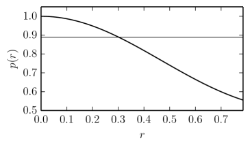
Figure 2: Expected payoff of Alice and Bob as a function of Bob‘s acceleration. The thin horizontal line is the classical threshold. The lines intersect for $r=\tan^{-1}\left(\sqrt{\frac{1}{3}\left(2\sqrt{7}-5\right)}\right)\approx 0.302171$.

5 Summary

We studied the quantum Magic Square game in a relativistic setup. We introduced formalism which takes into account the influence of the Unruh effect on the outcome of the game. Obtained results show that it is possible to achieve pseudo-telepathy for non-zero accelerations.

References

- [1] J. Eisert, M. Wilkens, and M. Lewenstein. Quantum games and quantum strategies. Physical Review Letters, 83(15):3077–3080, 1999.
- [2] S. C. Benjamin and P. M. Hayden. Comment on ’’Quantum Games and Quantum Strategies‘‘. Phys. Rev. Lett., 87(6):069801, 2001.
- [3] E. W. Piotrowski and J. Sładkowski. An invitation to quantum game theory. International Journal of Theoretical Physics, 42(5):1089–1099, 2003.
- [4] G. Brassard, A. Broadbent, and A. Tapp. Quantum pseudo-telepathy. Foundations of Physics, 35(11):1877–1907, 2005.
- [5] P. Gawron, J. A. Miszczak, and J. Sładkowski. Noise Effects in Quantum Magic Squares Game. International Journal of Quantum Information, 06(Supp):667, 2008.
- [6] Ł. Pawela, P. Gawron, Z. Puchała, and J. Sładkowski. Enhancing pseudo-telepathy in the magic square game. PloS one, 8(6):e64694, 2013.
- [7] N. D. Mermin. Simple unified form for the major no-hidden-variables theorems. Physical Review Letters, 65(27):3373–3376, 1990.
- [8] P. K. Aravind. Quantum mysteries revisited again. American Journal of Physics, 72:1303, 2004.
- [9] P. M. Alsing, I. Fuentes-Schuller, R. B. Mann, and T. E. Tessier. Entanglement of Dirac fields in noninertial frames. Physical Review A, 74(3):032326, 2006.
- [10] M. Aspachs, G. Adesso, and I. Fuentes. Optimal quantum estimation of the Unruh-Hawking effect. Physical review letters, 105(15):151301, 2010.
- [11] E. Martin-Martinez, L. J. Garay, and J. León. Quantum entanglement produced in the formation of a black hole. Physical Review D, 82(6):064028, 2010.
- [12] D. E. Bruschi, J. Louko, E. Martin-Martinez, A. Dragan, and I. Fuentes. Unruh effect in quantum information beyond the single-mode approximation. Physical Review A, 82(4):042332, 2010.
- [13] W. G. Unruh. Notes on black-hole evaporation. Physical Review D, 14(4):870, 1976.
- [14] P. C. W. Davies. Scalar production in Schwarzschild and Rindler metrics. Journal of Physics A: Mathematical and General, 8(4):609, 1975.