Micro-strip ferromagnetic resonance study of strain-induced anisotropy in amorphous FeCuNbSiB film on flexible substrate

Abstract

The magnetic anisotropy of a FeCuNbSiB (Finemet®) film deposited on Kapton® has been studied by micro-strip ferromagnetic resonance technique. We have shown that the flexibility of the substrate allows a good transmission of elastic strains generated by a piezoelectric actuator. Following the resonance field angular dependence, we also demonstrate the possibility of controlling the magnetic anisotropy of the film by applying relatively small voltages to the actuator. Moreover, a suitable model taking into account the effective elastic strains measured by digital image correlation and the effective elastic coefficients measured by Brillouin light scattering, allowed to deduce the magnetostrictive coefficient. This latter was found to be positive $(\lambda=16\times 10^{-6}$) and consistent with the usually reported values for bulk amorphous FeCuNbSiB.

I Introduction

The strain control of magnetization orientation distribution in magnetic thin films via the magnetoelastic or the magnetostrictive properties, is increasingly studied to face new challenges in magnetoelectronics and spintronics Nan2011_Adv_Mat ; Ramesh2010_Adv_Mat ; Martins2013_Adv_Func_Mater ; Roy2011 ; Ma2011 ; Lahtinen2011 . An easy way for mastering the magnetization is to make adhering the thin film on a piezoelectric actuator, so that the strains can be applied to the film by varying continuously a voltage on the piezoelectric actuator. This latter will succeed in transferring the strains in a more or less efficient way, depending on the chosen system. Obviously, more the elastic strains are transferred at the interface, more the indirect magnetoelectric effect is optimized. Generally, at a first step, the magnetic thin films are deposited on a substrate of usually one hundred microns thick. At a second step the film/substrate is cemented on an actuator Pettiford2008 ; Zighem_JAP2013 ; Brandlmaier2008_PRB ; Tiercelin2011 . At this point two interfaces will play their role in the transmission of strains: the actuator/substrate interface and the substrate/film one. This double transfer limits the desired phenomenon, especially when the substrate is stiff such as for commonly used wafer (Si, GaAs, …) Brandlmaier2008_PRB_Bis . Besides, in this configuration, it is generally hard to predict perfectly the amount of the induced strains inside the thin film ($\varepsilon_{xx}$ and $\varepsilon_{yy}$) even if the piezoelectric coefficients $d_{ijk}$ of the actuator are known. This is due to the partial strains transmissions from the actuator to the substrate, especially in the case of stiff substrates. This well-known reported limitation (a few ten percents of losses in best cases) can be avoided by depositing the magnetic thin film on a compliant substrate such as polyimides that are more and more used in flexible spintronics Barrault2012 ; Bedoya-Pinto2014 ; ZhangJAP2013_Bis . More precisely we reported in Ref. Zighem_JAP2013 , by comparing film and actuator strains, that one advantage of studying thin films on polymer substrates is the very good strains transmissions (nearly 100%) resulting from the substrate compliance. However, once well-known strains are transferred to the film, the estimation of the stresses ($\sigma_{xx}$ and $\sigma_{yy}$) is straightforward only if the elastic coefficients of this latter are known. Otherwise Hook’s law is not applicable. Unfortunately, the elastic coefficients are not always well-known, this is especially not the case when studying thin film of new functional alloys.

In this paper, voltage induced strain effect on the in-plane magnetic anisotropy has been quantitatively studied in a ferromagnetic film deposited on a flexible substrate and glued onto a piezoelectric actuator. In particular, the structural (Young’s modulus $E$ and Poisson’s ratio $\nu$) and magnetoelastic (magnetostriction coefficient at saturation $\lambda$) properties have been completely determined by combining different techniques. Our general methodology is based on the combination from one hand of i) the control of the applied stress state in a magnetic thin film and from another hand on ii) the magnetic uniform precession mode resonance field measurement as function of the stress. In order to control the stress state in the magnetic film, the film/substrate system is glued onto a piezoelectric actuator that allows applying in-plane strains ($\varepsilon_{11}$ and $\varepsilon_{22}$) when applying voltage to the actuator as it is shown on Figure 1. To properly estimate the in-plane strains by the double interfaces, we adopted the Digital Image Correlation (DIC) technique based on the optical observation of the film surface and its evolution during the film straining (section IV).

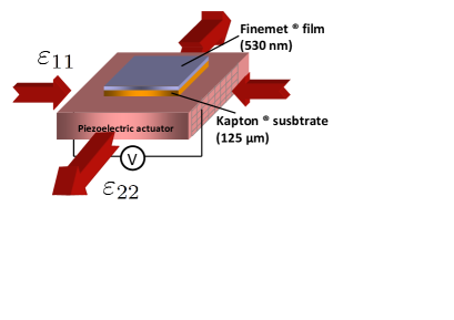
Figure 1: Sketch of the studied heterostructure showing the 530 nm thick Finemet® film deposited onto a 125 µm thick Kapton® substrate and glued onto the piezoelectric actuator. The arrows qualitatively represent the in-plane strains of the piezoelectric actuator.

A non-destructive method (Brillouin light scattering Rossignol2004 ; Fillon2014 ; Pham2013 ) has been used to quantify the elastic coefficients of the amorphous magnetic thin film (BLS study in section III). The magnetic anisotropy dependence upon the applied stress has been followed by measuring the behavior of the high frequency resonance field while applying an electric field inside the actuator. This resonance field is directly linked to the magnetic anisotropy and it can be estimated by performing Micro-Strip FerroMagnetic Resonance (MS-FMR )belmeguenai2009 ; belmeguenai2013 experiments in several geometrical configurations (section IV). Moreover, by adjusting an appropriate model (section II) to the experimental data, we have shown how to estimate with accuracy the thin film effective magnetostriction coefficient at saturation ($\lambda$).

II theoretical background

The voltage-induced strain effect has been experimentally studied by ferromagnetic resonance through uniform precession mode resonance field as a function of the applied voltage. Indeed, the resonance field (or resonance frequency) of the uniform precession mode is influenced by the magnetoelastic behavior of the thin film. All the experimental spectra presented in this work have been performed at room temperature. Moreover, they have been done at relatively “high” applied magnetic field in order to have a uniform magnetization inside the film. The expression of the resonance field is derived taking into account in-plane strains ($\varepsilon_{xx}$ and $\varepsilon_{yy}$). These in-plane strains will be induced by applying an electric field inside the piezoelectric actuator. When any magnetoelastic contribution is required, the magnetic energy density of a ferromagnetic thin film, using the coordinates system of 2, can be written as:

$$F_{0}=F_{zee}+F_{dip}+F_{exch}+F_{anis}$$ (1)

Where the three first terms stand for the Zeeman, the dipolar and the exchange contributions, respectively. The last term, which corresponds to the anisotropy contribution, will be written as an ad hoc in-plane uniaxial anisotropy characterized by the anisotropy constant $K_{u}$. This is correct when no out-of-plane or surface contributions to the anisotropy are observed in the film. This term can then be written as:

$$F_{anis}=-\frac{K_{u}}{M_{s}^{2}}\left(\vec{M}\cdot\vec{u}_{x}\right)^{2}$$ (2)

$\vec{u}_{x}$ is a unit vector along the “easy axis” (along $x$ direction) while $\vec{M}$ and $M_{s}$ are respectively the vector and the module of the magnetization. The stress effect will be modeled through a magnetoelastic density of energy $F_{me}$ which will be added to $F_{0}$:

$$F_{me}=-\frac{3}{2}\lambda\left(\left(\gamma_{x}^{2}-\frac{1}{3}\right)\sigma_{xx}+\left(\gamma_{y}^{2}-\frac{1}{3}\right)\sigma_{yy}\right)$$ (3)

$\sigma_{xx}$ and $\sigma_{yy}$ being the in-plane principal stress tensor components while $\gamma_{x}$ and $\gamma_{y}$ correspond to the direction cosines of the in-plane magnetization. The presence of a unique saturation magnetostriction coefficient $\lambda$ is due to the amorphous structure of the thin film. The relation between the principal stress components ($\sigma_{xx}$, $\sigma_{yy}$ ) and strains ($\varepsilon_{xx}$, $\varepsilon_{yy}$) tensors is thus given by an isotropic Hook’s law where $E$ is the Young’s modulus and $\nu$ is the Poisson’s ratio:

$$\sigma_{xx} =\left(\frac{E}{1+\nu}\right)\left(\frac{1}{1-\nu}\varepsilon_{xx}+\frac{\nu}{1-\nu}\varepsilon_{yy}\right)$$ (4)

$$\sigma_{yy} =\left(\frac{E}{1+\nu}\right)\left(\frac{1}{1-\nu}\varepsilon_{yy}+\frac{\nu}{1-\nu}\varepsilon_{xx}\right)$$ (5)

In these conditions, minimizing the total volume magnetic energy density (i. e. $F=F_{0}+F_{me}$), the resonance field of the uniform precession mode can be obtained thanks to the following relation Smit_Beljers_1955 ; Suhl_1955 :

$$\left(\frac{2\pi f}{\gamma}\right)^{2}=\left(\frac{1}{\sin\theta_{M}}\right)^{2}\left(\frac{\partial^{2}F}{\partial\theta_{M}^{2}}\frac{\partial^{2}F}{\partial\varphi_{M}^{2}}-\left(\frac{\partial^{2}F}{\partial\theta_{M}\varphi_{M}}\right)^{2}\right)$$ (6)

Where $f$ is the microwave driving frequency. The different energy derivatives are calculated at the equilibrium direction of the magnetization. In the above expression, $\gamma$ is the gyromagnetic factor $\gamma=g\times 8.794\times 10^{6}$ s^-1.Oe^-1 while $\theta_{M}$ and $\varphi_{M}$ stand for the polar and the azimuthal angles of the magnetization. Note that for an in-plane applied magnetic field, the equilibrium polar angle is $\varphi_{M}=\frac{\pi}{2}$ because of the large effective demagnetizing field associated with the planar film geometry and an explicit expression is obtained for $f$:

$$f^{2}=\left(\frac{\gamma}{2\pi}\right)^{2}H_{1}H_{2}$$ (7)

where:

$$H_{1} =4\pi M_{s}+H_{res}\cos\left(\varphi-\varphi_{H}\right)+\frac{2K_{u}}{M_{s}}\cos^{2}\varphi+\frac{3\lambda}{M_{s}}\left(\sigma_{xx}\cos^{2}\varphi+\sigma_{yy}\sin^{2}\varphi\right)$$ (8)

$$H_{2} =\left(\frac{2K_{u}}{M_{s}}+\frac{3\lambda}{M_{s}}\left(\sigma_{xx}-\sigma_{yy}\right)\right)\cos 2\varphi+H_{res}\cos\left(\varphi-\varphi_{H}\right)$$ (9)

Here $\varphi_{H}$ is the angle between the in-plane applied magnetic field and the magnetic easy axis ($x$ direction). The analysis can be simplified if the resonance field is larger than the effective uniaxial anisotropy and magnetoelastic field: $\vec{H}_{u}=-\vec{\nabla}_{\vec{M}}F_{anis}$ and $\vec{H}_{me}=-\vec{\nabla}_{\vec{M}}F_{me}$, respectively. Indeed, in this condition, the magnetization direction will be almost parallel to the applied magnetic field ($\varphi_{M}\sim\varphi_{H}$). The resonance field is thus given by:

$$H_{res}=\frac{1}{2}\left(\sqrt{\left(4\pi M_{s}+\left(H_{u}+\frac{3\lambda}{M_{s}}\sigma_{xx}\right)\sin^{2}\varphi+\frac{3\lambda}{M_{s}}\sigma_{yy}\cos^{2}\varphi_{H}\right)^{2}+4\left(\frac{2\pi f}{\gamma}\right)^{2}}-4\pi M_{s}\right)\\ -H_{u}\left(\frac{1}{4}+\frac{3}{4}\cos 2\varphi_{H}\right)-\frac{3\lambda}{M_{s}}\sigma_{xx}\left(\frac{1}{4}+\frac{3}{4}\cos 2\varphi_{H}\right)-\frac{3\lambda}{M_{s}}\sigma_{yy}\left(\frac{1}{4}-\frac{3}{4}\cos 2\varphi_{H}\right)$$ (10)

The first term essentially represents a constant shift in the resonance field baseline because $4\pi M_{s}$ and $\frac{2\pi f}{\gamma}$ are found to be larger than the magnetoelastic and the uniaxial anisotropy fields. The other terms correspond to the angular variation of the resonance field due to the uniaxial anisotropy field (second term) and to the voltage induced magnetoelastic anisotropy field (third and fourth terms).

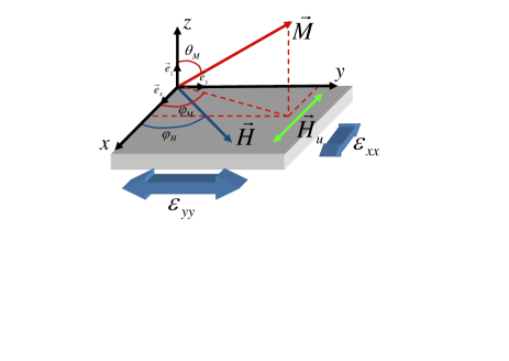
Figure 2: Schematic illustration showing angles, fields and coordinate systems used in the text.

III As-deposited thin film characterization at zero stress applied

III.0.1 Finemet thin film deposition and structure

An amorphous 530 nm thick Finemet® film was deposited onto a 125 $\mu$m thick polyimide flexible substrate (Kapton®) by radio frequency sputtering. The deposition residual pressure was of around 10^-7 mbar, while a working Ar pressure was of 40 mbar and the RF power was of 250 W. A 10 nm thick Ti buffer layer was deposited on the substrate to ensure a proper adhesion of the Finemet® film. Finally, another 10 nm thick Ti cap layer was deposited on the top of the Finemet® film in order to protect it from oxidation. The composition of the film has been measured by EDS (Energy Dispersive Spectroscopy) and is close to that of the target (Fe_73.5Cu₁Nb₃Si_15.5B₇) while the thickness of the film (530 nm) has been measured by Scanning Electron Microscopy and mechanical profilometry.

The film/substrate system has been then glued onto a piezoelectric actuator. Figure 1 presents a sketch of the studied heterostructure for studying the so-called inverse magnetoelectric effect. In this Figure $\varepsilon_{11}$ and $\varepsilon_{22}$ correspond to the in-plane strains at the surface of the actuator (top) and at the interface with the flexible substrate. This latter is again used here as it is the best possible medium for efficiently transfer the in-plane strain between the actuator and the ferromagnetic film. Maximum values of in-plane strains at a fixed voltage will be obtained as compared to those obtained when using a rigid substrate. Indeed, there is roughly two orders of magnitude between the Young’s modulus values of rigid substrates and the ones of a flexible one ($\sim$4 GPa for Kapton®) and $\sim$180 GPa for Si). Nevertheless, even if the interacting vector is the voltage induced in-plane strain transferred from the actuator to the ferromagnetic film, this is not sufficient to quantitatively analyze the indirect magnetoelectric effect. As stressed out in the previous section, in fact, the magnetoelastic anisotropy of the Finemet® material depends directly on the Young’s modulus $E$ and the Poisson’s ratio $\nu$ of the thin film. To determine them, we performed a Brillouin light scattering (BLS) study

III.0.2 Elastic coefficients estimation by Brillouin light scattering (BLS)

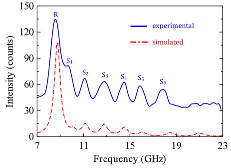
Figure 3: Brillouin light scattering spectrum of the amorphous Finemet® film on Kapton® substrate. The transferred wave-vector is $q=2.14\times 10^{5}$ cm^-1. $R$ denotes Rayleigh surface wave while $S_{i}$ correspond to the Sesawa guided waves. The red dashed line corresponds to the theoretical calculated spectrum while the continuous blue line corresponds to the experimental data.

During the last twenty years, BLS has proved to be very efficient for achieving a complete elastic characterization of thin films and multilayered structures Rossignol2004 ; Pham2013 ; Fillon2014 . In a BLS experiment, a monochromatic light beam probes and reveals acoustic phonons characteristic of the investigated medium. The power spectrum of these phonons is mapped out from the frequency analysis of the light scattered within a solid angle. Because of the wave vector conservation in the phonon-photon interaction, the wavelength of the revealed elastic waves is of the same order of magnitude as that of light. This means that the wavelength is much larger than the inter-atomic distances, so that the material can be described as a continuum within an effective-medium approach. The BLS spectra were collected in air at room temperature with typical acquisition times of a few hours. 30 mW p-polarized monochromatic light coming from a solid state laser ($\Lambda=532$ nm) was focused on the surface of the sample. We used back-scattering configuration and the scattered light was analyzed thanks to a (3+3)-pass tandem Fabry–Pérot interferometer, so that the value of the wave vector of the probed surface acoustic waves is experimentally fixed to the value $q=\frac{4\pi}{\lambda}\sin\left(\xi\right)=2.14\times 10^{5}$ rad.cm^-1, where $\xi=65\text{\textdegree}$ is the incidence angle of the light beam.

For nearly opaque films with thicknesses around the acoustic wavelength (0.3 - 0.4 $\mu$m), we can observe the surface acoustic waves with a sagittal polarization. The Rayleigh wave ($R$), the so-called Sesawa guided waves ($S_{1}$ to $S_{i}$) and the corresponding phase velocities are then measured. In our case, the amorphous film can be considered as isotropic. Thus, two isotropic elastic coefficients (Young’s modulus $E$ and Poisson’s ratio $\nu$ of the thin amorphous film) influence the Rayleigh and Sezawa modes, so that they can be evaluated by a best fit procedure of the experimental velocities to the calculated dispersion curves. By taking into account only the ripple mechanism for the scattered intensity by the surface acoustic waves, the experimental spectra are well fitted, leading to the following values : $E=145\times 10^{10}$ dyn.cm^-2 ($\equiv 145$ GPa) and $\nu=0.27$. The estimated Young’s modulus is close to the one of amorphous bulk FeCuNbSiB rubbans Kobelev1998 .

III.0.3 Magnetic parameters at zero applied voltage

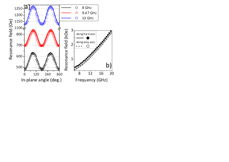
Figure 4: a) In-plane angular ($\varphi_{H}$) dependence of the resonance field at three different driven frequencies (8, 9.47 and 12 GHz). b) Variation of the uniform precession resonance field variation as a function of the microwave driven frequency $f$ at zero applied voltage. Open symbols are obtained with $\varphi_{H}=0$ (easy axis: $\vec{H}\parallel\vec{e}_{x}$) and the filled ones are obtained with $\varphi_{H}=\pi/2$ (hard axis: $\vec{H}\parallel\vec{e}_{y}$). The solid and dashed lines in a) and b) are best fits to the experimental data using equation 10 with the following parameters: $\gamma=1.885\times 10^{7}$ Hz.Oe^-1, $M_{S}=965$ emu.cm^-3, $K_{u}=3.8\times 10^{4}$ erg.cm^-3 and $\sigma_{xx}=\sigma_{yy}=0$.

During this study, the magnetic properties have been probed by using Micro-Strip FerroMagnetic Resonance (MS-FMR) which is now a common technique to scrutinized the dynamic magnetic properties in the microwave regime. This setup allows the determination of the resonance field $H_{res}$ of the uniform precession mode by sweeping the applied magnetic field in presence of a fixed pumping radio frequency field $\vec{h}_{rf}$ (i. e. microwave driving frequency $f$).

In order to enhance the signal to noise ratio, a weak modulation of the static applied magnetic field (here $\sim 5$ Oe at 175 Hz) is performed. Thus, this setup gives access to the field first derivative of the rf absorption as a function of the applied magnetic field. We have first studied the magnetic properties of the Finemet® thin film in zero-applied voltage. The angular ($\varphi_{H}$) dependence of the resonance field has been studied for different microwave driving frequency $f$. This dependence is presented in Figure 4a) for three frequencies (8, 9.47 and 12 GHz). Note that the measurements performed at 9.47 GHz have been performed by using a resonant cavity thanks to an Electron Paramagnetic Resonance (EPR) set-up and are clearly consistent with the MS-FMR ones. All the measurements show that the angular dependencies are governed by a uniaxial anisotropy having an easy axis along $x$ direction (the resonance field is indeed minimum at $\varphi_{H}=0$). Figure 4b) presents the resonance field variation as function of the microwave driving frequency $f$ along the easy axis ($\varphi_{H}=0$, open circles) and along the hard axis ($\varphi_{H}=\frac{\pi}{2}$, filled circles). The continuous lines in Figure 4 are calculated thanks to equation 10. The in-plane strains are equal to zero ($\varepsilon_{xx}(V=0)=\varepsilon_{yy}(V=0)=0$) in absence of applied voltage and therefore the resonance field depends only on $\gamma$, $M_{s}$ and $K_{u}$ Zighem2010 . The best fits to experimental data are obtained using the following parameters: $\gamma=1.885\times 10^{7}$ s^-1.Oe^-1, $M_{S}=965$ emu.cm^-3 (i. e. $4\pi M_{s}\sim 12100$ G) and $K_{u}=3.8\times 10^{4}$ erg.cm^-3(i. e. $H_{u}\sim 80$ Oe). The obtained Landé factor ($g\sim 2.1)$ value is the typical for metallic ferromagnets and the $M_{s}$ value is in a good agreement with previously determined values for similar films. However, due to the amorphous structure of the material, the in-plane magnetic anisotropy in equivalent Finemet® film deposited onto rigid substrate (Si) is generally weaker (a few Oe) than the $\sim 80$ Oe found here. As previously suggested ZhangJAP_2013 ; ZhangAPL_2013 ; Gueye2014 ; Gueye2014_BIS , the origin of this uniaxial anisotropy is certainly due to a non zero magnetoelastic anisotropy at zero-applied voltage. This “initial” anisotropy can be due to a slight curvature along a given direction taking place during the elaboration process which could lead to a magnetoelastic anisotropy at zero-applied voltage. Thereafter, this residual anisotropy will be modeled as an ad hoc uniaxial one.

IV Magnetic anisotropy strains effect

IV.1 Measured in-plane strains

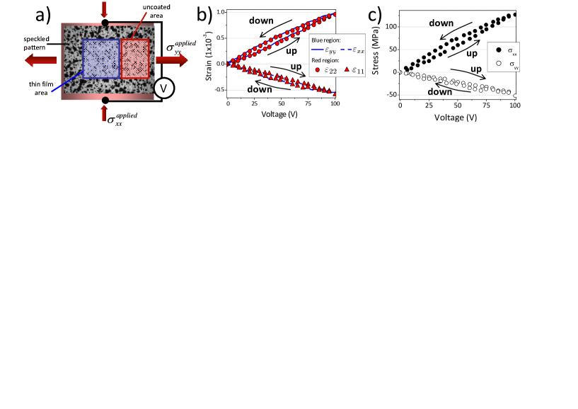
Figure 5: a) Top view sketch of the system showing the spray-painted speckle pattern in order to generate a contrast at the surface of the film. The blue and red areas correspond to the top surface of the film region and to an uncoated area of the actuator, respectively. b) Extracted mean in-plane strains from the blue (film surface) and red (uncoated actuator surface) areas by performing DIC calculations. Continuous lines correspond to $\varepsilon_{xx}$ and $\varepsilon_{yy}$ while and symbols correspond to $\varepsilon_{11}$ and $\varepsilon_{22}$. c) Calculated mean in-plane stresses $\sigma_{xx}$ and $\sigma_{yy}$ using equations 4 and 5 with $E=145\times 10^{10}$ dyn.cm^-2 and $\nu=0.27$. In b) and c), the applied external voltage was swept from 0 V to 100 V and back to 0 V with steps of around 5 V. The first measurement at 0 V has been performed after “saturating” the actuator at 100 V to avoid training effect of the actuator polarization.

The piezoelectric actuator is characterized by a main axis direction (direction 2 in Figure 1). The film/substrate system has been glued in order to have the main deformation axis of the actuator perpendicular to the easy axis, so in this condition, the direction $1$ (resp. $2$) of the actuator refers to $x$ (resp. $y$) direction of the thin film. Digital image correlation (DIC) method enables accurate measurements of changes in digital images Haddadi2012 ; Djaziri2011 . This method uses tracking and image registration to make full-field non-contact measurements of displacements and strains in a wide variety of engineering applications (mechanics of materials, micro- and nano-technology, …). Here, two CCD cameras mounted on a tripod have been positioned vertically in top of the film/substrate/actuator system, the field of view is fixed to approximately $2\times 2$ cm². Given the $2448\times 2050$ number of pixels of the cameras, the area per pixel is about $12.5$ nm². The respective positions of the cameras has been calibrated by using a 10 mm$\times$8 mm calibration pattern. Figure 5a) presents a part speckle pattern which has been generated at the “uniform” top surface of the heterostructure by using a spray paint in order to generate a contrast which will serve to calculate the deformation. Indeed, a first image (reference image) is taken at zero applied voltage; then, a sequence of images are taken at different applied voltages and are compared to the reference. The field strain at the surface of the system has been extracted for each applied voltage by performing DIC calculations which are performed by using the reference image and the different images coming from the sequence. The DIC calculations have been performed by using ARAMIS which is a commercially available software package Aramis . From the fields strain, the mean in-plane strains are extracted as function of the applied voltage. Note that shear strains can also be extracted because of the use of two cameras in the present setup. However, the shear strains values are found to be negligible in this study and will be neglected thereafter.

Images were collected by performing applied voltage loops (from 0V to 100V and back to 0V) with a frame rate of about 0.1 FPS; the step of applied voltage was fixed to around 5 V. Furthermore, prior to the measurements, several images have been taken in absence of voltage in order to estimate the DIC setup statistical errors, estimated to be $\sim 5\times 10^{-6}$. Moreover, different images have been taken as a function of time at 0 V after saturating the actuator at 100 V. After approximately 5 hours, a difference of about $\left|4\times 10^{-5}\right|$ in the in-plane strains values is found; this value rises to $\left|1\times 10^{-4}\right|$ after several days (which is relatively high). This difference is due to the training effect of the polarization. In addition, ARAMIS has been used to calculate the DIC in two different $3\times 3$ mm² regions: an uncoated area of the actuator and an area located at the top of the thin film.

Figures 5b) presents the extracted mean in-plane strains $\varepsilon_{11}$ and $\varepsilon_{22}$. Indeed, similar quasi-homogeneous strain fields as function of the applied voltage have been calculated from the two regions. Thus a $100\%$ in-plane strain transmission in between the piezoelectric actuator and the film is observed, it can be conclude that $\varepsilon_{11}=\varepsilon_{xx}$ and $\varepsilon_{22}=\varepsilon_{yy}$. Non linear and hysteretic variations are observed for both $\varepsilon_{11}$ and $\varepsilon_{22}$ which is certainly due to the intrinsic properties of the ferroelectric material used in the fabrication of the actuator Zighem_JAP2013 . One can note that $\varepsilon_{22}$ is found to be positive and $\varepsilon_{11}$ is found to be negative in the voltage range [0-100 V]. Moreover, it is interesting to note that a linear variation of $\varepsilon_{22}$ as a function of $\varepsilon_{11}$ is found $\varepsilon_{22}\simeq-1.7\varepsilon_{11}$. The maximum achieved values of $\varepsilon_{22}$ and $\varepsilon_{11}$ ($\sim 1\times 10^{-3}$ $\sim-0.5\times 10^{-3}$ at 100 V, respectively) show that the film is not deteriorated by the plasticity regime because it is obtained for higher values: this is experimentally confirmed by the excellent reproducibility of the experiments (even after several days). In this condition and because of the amorphous structure of the magnetic film, the in-plane stresses can be calculated using equations 4 and 5 with $E$ and $\nu$ values previously determined by BLS. Obviously, $\sigma_{11}$ and $\sigma_{22}$ also present non linear and hysteretic variations as function of the applied voltage. This representation of the in-plane stresses could be useful, especially in the case of uniaxial in-plane stress which is not the case here. Indeed, for $\sigma_{22}$ , a similar linear variation is found with $\sigma_{22}\simeq-3.6\sigma_{11}$.

From the voltage dependence of $\varepsilon_{11}$ and $\varepsilon_{22}$ (or $\sigma_{11}$. and $\sigma_{22}$), the indirect magnetoelectric effect can be quantitatively studied in the the system by probing resonance field uniform mode.

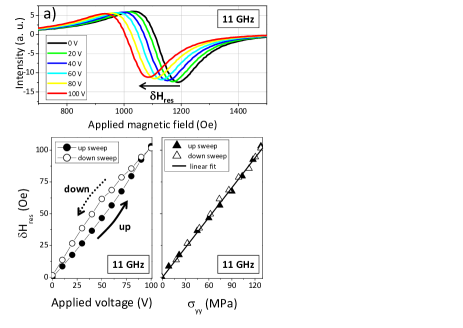
Figure 6: a) Experimental spectra recorded at 11 GHz with $\varphi_{H}=\frac{\pi}{2}$ at different applied voltages. (b) Resonance field variations (at 11 GHz and $\varphi_{H}=0$) as a function of the applied voltage (b) and of the applied stress (c). The open symbols correspond to upsweep (0 to 100 V) while filled symbols correspond to downsweep (100 to 0 V). Note that $\delta H_{res}$ hysteresis disappears when the data are plotted as function of $\sigma_{yy}$ (or $\sigma_{xx}$). The solid lines in Figure 7b are guided for the eyes while the solid line in Figure 7c corresponds to a linear fit.

	$\alpha_{me}$ (V.cm-1.Oe-1)		$\alpha_{ms}^{\sigma_{yy}}$ (Oe.MPa-1)
$f$ (GHz)	$\varphi_{H}$
	$0$	$\frac{\pi}{2}$	$0$	$\frac{\pi}{2}$
8	-1.62	1.4	-0.67	0.77
10	-1.62	1.39	-0.62	0.77
11	-1.76	1.41	-0.63	0.77
12	-1.68	1.41	-0.64	0.76
13	-1.7	1.4	-0.58	0.75
14	-1.76	1.41	-0.62	0.76
15	-1.85	1.44	-0.58	0.75
16	-1.81	1.76	-0.59	0.62
18	-1.81	1.7	-0.6	0.64
20	-1.831	1.37	-0.6	0.79

Table 1: $\alpha_{me}$ and $\alpha_{ms}^{\sigma_{yy}}$ as function of the microwave driving frequency $f$ extracted along the $x$ and $y$ direction.

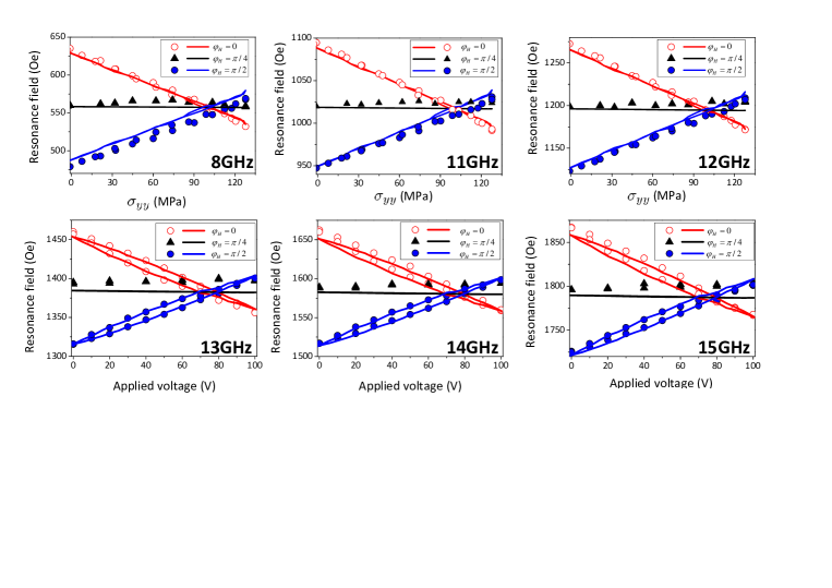
Figure 7: Resonance field variation as a function of the induced in-plane stress $\sigma_{22}$ (top graphs) and the applied voltage (down graphs) measured at different microwave driven frequencies (8-15 GHz) and in-plane angular angles ($\varphi_{H}$=0, $\frac{\pi}{2}$ and $\frac{\pi}{4}$). Note that the observed hysteretic and non linear variations (see Figure 6 disappears). Open circles are obtained with $\varphi_{H}=0$ (initial easy axis: $\vec{H}\parallel\hat{x}$), the filled circles are obtained with $\varphi_{H}=\frac{\pi}{2}$ (hard axis: $\vec{H}\parallel\hat{y}$) and the open triangles are obtained with $\varphi_{H}=\frac{\pi}{4}$. The different lines are best fits to the experimental data using equation 10 with the following parameters: $\gamma=1.885\times 10^{7}$ s^-1.Oe^-1, $M_{S}=965$ emu.cm^-3, $K_{u}=3.8\times 10^{4}$ erg.cm^-3, $E=145$ GPa and $\nu=0.27$ and $\lambda=16\times 10^{-6}$.

IV.2 Strain induced anisotropy and magnetoelastic behavior

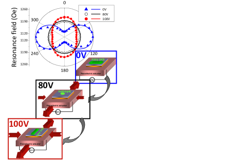
Figure 8: In-plane angular ($\varphi_{H}$) dependence of the resonance field measured at 12 GHz for three different applied voltages: 0, 80 and 100 V. The symbols are experimental data (triangles: 0 V, open circles: 80 V and filled circles: 100 V) while the solid lines are calculated thanks to equation 10 with the following parameters: $\gamma=1.885\times 10^{7}$ s^-1.Oe^-1, $M_{S}=965$ emu.cm^-3, $K_{u}=3.8\times 10^{4}$ erg.cm^-3, $E=145\times 10^{10}$ dyn.cm^-2 and $\nu=0.27$ and $\lambda=16\times 10^{-6}$. The Sketches correspond to 3D view of the heterostructure showing the voltage-switch of the easy axis from $x$ to $y$ direction.

Figures 6a) shows typical MS-FMR experimental spectra recorded at 11 GHz with an applied magnetic field along $y$ direction (initial hard axis: $\varphi_{H}=\frac{\pi}{2}$) at different applied voltages (0, 20, 40, 60, 80 and 100 V). A shift of the resonance field $\delta H_{res}$ of around 100 Oe between spectra recorded at 0 and 100 V is clearly obvious. The corresponding variation of $\delta H_{res}$ (defined as $\delta H_{res}=H_{res}(0)-H_{res}(V)$) as a function of the applied voltage is reported in Figure 6: a non linear and hysteretic variation is observed. Here, filled circles represent the upsweep (0 to 100 V) and open circles the downsweep of the applied voltage (100 to 0 V). The spectra presented in Figure 6a) show that the resonance field decreases when increasing the applied voltage. Since $\varepsilon_{yy}>0$ and $\varepsilon_{xx}<0$, it can be conclude that the magnetostriction coefficient at saturation $\lambda$ of the thin film is positive. Indeed, a negative magnetostriction coefficient would have led to an increase of $H_{res}$, as it is the case in Ni polycrystalline thin film Zighem_JAP2013 ; BrandlmaierNewJ.Phys_2009 .

Furthermore, a linear variation of $\delta H_{res}$ appears if the voltage-stress dependence (see Figure 5) is used. Figure 6c) illustrates such a behavior where the continuous line is the linear fit of the slope which is found around $\alpha_{ms}^{\sigma_{yy}}=0.76$ Oe.MPa^-1. This feature indicates that the non linear and the hysteretic variations of $\delta H_{res}$ as a function of $V$ is not related to the magnetoelastic anisotropy; it is completely due to the intrinsic properties of the ferroelectric material used for the actuator fabrication. In addition, in first approximation, if the non linear and the hysteretic behavior of $\delta H_{res}$ as a function of $V$ is neglected and adjusted by a linear fit, an effective magnetoelectric coupling ($\alpha_{me}$ in V.cm^-1.Oe^-1 ) can be estimated (by considering the static electric field inside the actuator. Table 1 presents the different values of $\alpha_{me}$ and $\alpha_{ms}^{\sigma_{yy}}$ as function of the microwave driving frequency measured along the initial easy and hard axes ($\varphi_{H}=0$ and $\frac{\pi}{2}$). The first observation is that the voltage-induced magnetoelastic effect is frequency independent for this system. However, a weak difference of $\alpha_{me}$ extracted from the measurements performed at $\varphi_{H}=0$ and $\varphi_{H}=\frac{\pi}{2}$ is found. Such effect is most probably due to the misalignment (of a few degrees) of the $x$ direction and the direction $1$ of the actuator which may occurred when gluing of the film/substrate system onto the piezoelectric actuator and is predicted by the equation 10.

Figure 7 presents variations of $H_{res}$ as a function of the applied voltage-induced stress (three top graphs) and as a function of the applied voltage (three down graphs) for different $\varphi_{H}$ angles ($0$, $\frac{\pi}{4}$ and $\frac{\pi}{2}$) at various microwave driving frequencies. In first approximation, the induced magnetoelastic anisotropy can be viewed as a uniaxial magnetoelastic anisotropy field $\vec{H}_{me}$ along $y$ direction, which is thus perpendicular to the “initial” uniaxial anisotropy field $\vec{H}_{u}$. In absence of applied voltage, the resonance field along $x$ direction ($\varphi_{H}=0$) is smaller than the one measured along $y$ direction ($\varphi_{H}=\frac{\pi}{2}$), the difference of these two last resonance fields is roughly equal to $\left\|2\vec{H}_{u}\right\|$. When increasing the applied voltage (or induced-stress), the $x$ direction will be less easy which leads to an increase (resp. decrease) of the resonance field along $x$ (resp. along $y$) direction because of the competition between $\vec{H}_{me}$ and $\vec{H}_{u}$. At 80 V ($\sigma_{11}\sim-30$ MPa and $\sigma_{22}\sim 105$ MPa), the resonance fields are equal for the three studied angles which means that $\vec{H}_{u}$ is totally compensated by $\vec{H}_{me}$. A quantitative analysis of the voltage-induced variation of the resonance field has been performed by using equation 10. By introducing the stress-voltage dependence, the only undetermined parameter is the saturation magnetostriction coefficient $\lambda$; the best fits of all the experiments gives $\lambda=16\times 10^{-6}$, which is slightly lower with the bulk material. A good agreement is found between the experimental variations and the calculated ones for the different frequencies (see 7). Note that the non linear and the hysteretic variations of $H_{res}$ as a function of $V$ are well reproduced. In addition, at $\varphi_{H}=\frac{\pi}{4}$, an experimentally confirmed almost constant variation as predicted by equation 10.

Figure 8 presents angular variations of the resonance field at different applied voltage: 0, 80 and 100V which correspond to $\sigma_{11}\sim 0$, -30 and -45 MPa and $\sigma_{22}\sim 0$, 105 and 130 MPa, respectively. At zero-voltage, the angular variation of the resonance field found in Figure 4a) is retrieved, the horizontal peanut shape represented by blue triangles is characteristic of a uniaxial anisotropy along $x$ direction ($\varphi_{H}=0$). The 80 V value was chosen because of the “exact” compensation of this uniaxial anisotropy by the induced magnetoelastic one. At this voltage, the film is in-plane isotropic in the magnetic point of view. It is experimentally confirmed by the circle shape formed by the open circles. Finally, at 100 V, a uniaxial anisotropy characterized by a vertical peanut shape is observed along $y$ axis ($\varphi_{H}=\frac{\pi}{2}$). Thus, a voltage-switch of the effective easy axis from $x$ direction (at 0 V) to $y$ direction (at 100 V) has been performed. The sketches of Figure 4b qualitatively present such effect. Finally, the solid lines of Figure 4a are calculated thanks to equation 10 with the parameters previously determined.

V Conclusions

• Magnetic anisotropy in Finemet® thin films deposited on Kapton® substrate has been studied by Micro-Strip FerroMagnetic Resonance (MS-FMR).

• We have shown that the flexibility of Kapton® substrate allowed tailoring the magnetic anisotropy of the film by applying small voltage-induced strains.

• The flexibility of the Kapton® substrate induced an initial uniaxial anisotropy that is generally not found in ferromagnetic films whose thickness is a few hundred nanometers.

• The knowledge of the applied elastic strains versus applied voltage measured by Digital Image Correlation and Finemet® film elastic constants measured by Brillouin light Scattering allowed estimating the effective magnetostriction coefficient of the film.

- (1) Jing Ma , Jiamian Hu , Zheng Li and Ce-Wen Nan, Adv. Mater. 23, 1062 (2011)
- (2) Carlos A. F. Vaz , Jason Hoffman , Charles H. Ahn and Ramamoorthy Ramesh, Adv. Mater., 22, 2900 (2010)
- (3) Pedro Martins and Senentxu Lanceros-Méndez, Adv. Funct. Mater., 23, 3371 (2013)
- (4) J. Ma, J. Hu, Z. Li, C.-W. Nan, Adv. Mater. 23, 1062-1087 (2011)
- (5) T. H. E. Lahtinen, J. O. Tuomi, S. van Dijken, Adv. Mater. 23, 3187-3191 (2011)
- (6) K. Roy, S. Bandyopadhyay, J. Atulasimha, Appl. Phys. Letters 99, 063108 (2011)
- (7) C. Pettiford, J. Lou, L. Russell, and N. X. Sun, App. Phys. Lett. 92, 122506 (2008)
- (8) C. Bihler, M. Althammer, A. Brandlmaier, S. Geprägs, M. Weiler, M. Opel, W. Schoch, W. Limmer, R. Gross, M. S. Brandt and S. T. B. Goennenwein, Phys. Rev. B 78, 045203 (2008)
- (9) F. Zighem, D. Faurie, S. Mercone, M. Belmeguenai and H. Haddadi, J. App. Phys. 114, 073902 (2013)
- (10) N. Tiercelin, Y. Dusch, A. Klimov, S. Giordano, V. Preobrazhensky and P. Pernod, App. Phys. Lett., 99, 192507 (2011)
- (11) A. Brandlmaier, S. Geprägs, M. Weiler, A. Boger, M. Opel, H. Huebl, C. Bihler, M. S. Brandt, B. Botters, D. Grundler, R. Gross and S. T. B. Goennenwein, Phys. Rev. B 77, 104445 (2008)
- (12) C. Barraud, C. Deranlot, P. Seneor, R. Mattana, B. Dlubak, S. Fusil, K. Bouzehouane, D. Deneuve, F. Petroff, and A. Fert, Appl. Phys. Lett. 96, 072502 (2010)
- (13) A. Bedoya-Pinto, M. Donolato, M. Gobbi, L. E. Hueso, Paolo Vavassori, App. Phys. Lett. 104, 062412 (2014)
- (14) Z. Zuo,1,2 Q.Zhan, G. Dai, B. Chen, X. Zhang, H. Yang, Y. Liu and R.-W. Li, J. Appl. Phys., 113, 17C705 (2013)
- (15) J. Smit, H.G. Beljers, Philips Res. Rep. 10, 113 (1955)
- (16) H. Suhl, Phys. Rev. 97, 555 (1955)
- (17) C. Rossignol, B. Perrin, B. Bonello, P. Djemia, P. Moch, H. Hurdequint, Phys. Rev. B 70, 094102 (2004)
- (18) A. Fillon, C. Jaouen, A. Michel, G. Abadias, C. Tromas, L. Belliard, B. Perrin, P. Djemia, Phys. Rev. B 88, 174104 (2014)
- (19) T. Pham, D. Faurie, P. Djemia, L. Belliard, E. Le Bourhis, P. Goudeau, F. Paumier, Appl. Phys. Letter 103, 041601 (2013)
- (20) M. Belmeguenai, F. Zighem, Y. Roussigné, S-M. Chérif, P. Moch, K. Westerholt, G. Woltersdorf and G. Bayreuther, Phys. Rev. B 79, 024419 (2009)
- (21) M. Belmeguenai, H. Tuzcuoglu, M. S. Gabor, T. Petrisor jr, C. Tiusan, D. Berling, F. Zighem, T. Chauveau, S. M. Chérif, P. Moch, Phys. Rev. B 87, 184431 (2013)
- (22) N.P Kobelev, Y. M. Soifer, Nanostructured Materials 10, 449-456 (1998)
- (23) Y. Yoshizawa, S. Oguma, and K. Yamauchi, J. Appl. Phys. 64, 6044 (1988)
- (24) G. Herzer, Physica Scripta T49, 307 (1993)
- (25) F. Zighem, Y. Roussigné, S. M. Chérif, P. Moch, J. Ben Youssef, and F. Paumier, J. Phys.: Condens. Matter. 22, 406001 (2010).
- (26) X. Zhang, Q. Zhan, G. Dai, Y. Liu, Z. Zuo, H. Yang, B. Chen, and R.-W. Li, J. Appl. Phys., 113, 17A901 (2013).
- (27) X. Zhang, Q. Zhan, G. Dai, Y. Liu, Z. Zuo, H. Yang, B. Chen and R.-W. Li, App. Phys. Lett., 102, 022412 (2013)
- (28) M. Gueye, F. Zighem, D. Faurie, M. Belmeguenai and S. Mercone, App. Phys. Lett., 105, 052411 (2014)
- (29) M. Gueye, B. M. Wague, F. Zighem, M. Belmeguenai, M. S. Gabor, T. Petrisor Jr, C. Tiusan, S. Mercone and D. Faurie, App. Phys. Lett., 105, 062409 (2014)
- (30) H. Haddadi and S. Belhabib, Int. J. of Mech. Sc. 62, 47 (2012)
- (31) S. Djaziri, P. O. Renault, F. Hild, E. Le Bourhis, P. Goudeau, D. Thiaudière, D. Faurie, J. Appl. Cryst. 44, 1071 (2011)
- (32) http://www.gom.com/
- (33) M. Weiler, A. Brandlmaier, S. Gepr€ags, M. Althammer, M. Opel, C. Bihler, H. Huebl, M. S. Brandt, R. Gross, and S. T. B. Goennenwein, New J. Phys., 11, 013021 (2009).