USAT: A Unified Score-based Association Test for Multiple Phenotype-Genotype Analysis

Abstract

Genome-wide Association Studies (GWASs) for complex diseases often collect data on multiple correlated endo-phenotypes. Multivariate analysis of these correlated phenotypes can improve the power to detect genetic variants. Multivariate analysis of variance (MANOVA) can perform such association analysis at a GWAS level, but the behavior of MANOVA under different trait models has not been carefully investigated. In this paper, we show that MANOVA is generally very powerful for detecting association but there are situations, such as when a genetic variant is associated with all the traits, where MANOVA may not have any detection power. We investigate the behavior of MANOVA, both theoretically and using simulations, and derive the conditions where MANOVA loses power. Based on our findings, we propose a unified score-based test statistic USAT that can perform better than MANOVA in such situations and nearly as well as MANOVA elsewhere. Our proposed test reports an approximate asymptotic p-value for association and is computationally very efficient to implement at a GWAS level. We have studied through extensive simulation the performance of USAT, MANOVA and other existing approaches and demonstrated the advantage of using the USAT approach to detect association between a genetic variant and multivariate phenotypes. We applied USAT to data from three correlated traits collected on $5,816$ Caucasian individuals from the Atherosclerosis Risk in Communities (ARIC, The ARIC Investigators (1989)) Study and detected some interesting associations.

1 Introduction

In the study of a complex disease, data on several correlated endo-phenotypes are often collected to get a better understanding of the disease. For example, in the study of thrombosis, the intermediate correlated phenotypes such as Factor VII, VIII, IX, XI, XII, and von Willebrand factor influence greatly the risk of developing thrombosis (Souto et al., 2000; Germain et al., 2011). An epidemiologic study on type 2 diabetes (T2D) typically collects data on a number of risk factors and diabetes-related quantitative traits. The standard approach to analyze these phenotypes is to perform single-trait analyses separately and report the findings for individual trait.

van der Sluis et al. (2013) demonstrated several alternative models which would benefit from a joint analysis. Blair et al. (2013) illustrated the comorbidity between Mendelian disorders and different complex disorders, which indicates that there may be common genetic variants affecting several of these complex traits. Recently, many articles advocating joint analysis over univariate analysis of multiple correlated traits (Ferreira and Purcell, 2009; Zhang et al., 2009; Korte et al., 2012; O’Reilly et al., 2012; Stephens, 2013; Aschard et al., 2014; Galesloot et al., 2014; Zhou and Stephens, 2014; Ried et al., 2014, and references therein) have been published that illustrate the benefits of jointly analyzing these correlated traits to improve the power of detection of genetic variants. Moreover this joint analysis could reveal some pleiotropic genes involved in the biological development of the disease.

Few approaches have been developed to perform association analysis with multivariate traits at a GWAS level. O’Reilly et al. (2012) proposed MultiPhen to detect association between multivariate traits and a single nucleotide polymorphism (SNP) with unrelated individuals. MultiPhen uses ordinal regression to regress a SNP on a collection of phenotypes and tests whether all regression parameters corresponding to the phenotypes in the model are significantly different from zero. It can accommodate both binary and continuous traits but may suffer from lack of power when a SNP is associated with all the highly correlated traits. van der Sluis et al. (2013) proposed Trait-based Association Test (TATES) for testing association between multiple traits and multiple SNPs using extended Simes procedure on the p-values derived from univariate trait and single SNP association analysis. Even when the phenotypes are strongly correlated, TATES gives appropriate type I error for varying minor allele frequency (m.a.f.). It may have low power when a SNP affects only a few of the strongly correlated traits. Maity et al. (2012) proposed a kernel machine method for unrelated individuals for joint analysis of multimarker effects on multiple traits. Kernel machine is a powerful dimension-reduction tool that can accommodate linear/non-linear effects of multiple SNPs. Their test for association between multiple SNPs and the phenotypes is equivalent to testing the variance components in a multivariate linear mixed model (mvLMM). Implementation of this approach requires parametric bootstrapping to estimate the distribution of the test statistic and could be computationally intensive at a GWAS level. Korte et al. (2012); Zhou and Stephens (2012) implemented mvLMM for GWAS. Zhou and Stephens (2014) explored efficient algorithms for mvLMM in a GWAS setting.

Recently, data reduction methods such as principal component analysis (PCA) and canonical correlation analysis (CCA) are being explored to perform multivariate association analysis (Tang and Ferreira, 2012; Basu et al., 2013; Aschard et al., 2014). The advantage of using CCA to perform gene-based tests on multivariate phenotypes has been elaborately discussed in Tang and Ferreira (2012); Basu et al. (2013). Previously, Ferreira and Purcell (2009) proposed a multivariate test of association based on CCA to simultaneously test the association between a single SNP and multiple phenotypes. Their CCA approach is equivalent to multivariate analysis of variance (MANOVA) or more generally the Wilk’s lambda test in multivariate multiple linear regression (MMLR) approach (Muller and Peterson, 1984). Basu et al. (2013) extended the MANOVA to family data. Both O’Reilly et al. (2012) and van der Sluis et al. (2013) found significantly high power for MANOVA when a subset of traits was associated with the causal variant or gene. One major advantage of MANOVA is that it can easily be extended to incorporate multiple phenotypes as well as multiple SNPs (such as a gene). Moreover other covariates can easily be incorporated in the model.

In this paper, we explore the performance of MANOVA to detect multi-trait association under various alternative trait models. Our simulation studies consider a single marker to investigate the properties of MANOVA. Further, we theoretically justify the behavior of MANOVA and provide a geometrical explanation as well. We demonstrate that MANOVA may lose significant power when the genetic marker is associated with all the traits and any test that does not consider the within trait correlation can have more power in such a situation. Utilizing these findings, we propose a novel unified score-based association test (USAT) that maintains good power under various alternative trait models and performs significantly better than MANOVA when all the traits are associated.

This paper evolves as follows. Section 2 describes some popular existing methods for doing association analysis using multiple phenotypes. More specifically, section 2.1 describes the univariate methods that completely ignore trait correlations, section 2.2 describes a method that accounts for the within trait correlation only through the distribution of the test statistic while section 2.3 describes a multivariate method that directly incorporates the trait correlation structure. Section 2.4 theoretically and geometrically justifies some aspects of the behavior of MANOVA, for $K$ traits and a single SNP, in situations that commonly arise in such genetic studies. Section 2.5 introduces our unified approach USAT for association analysis using multiple traits and a single marker for unrelated individuals. Section 3 illustrates a comparison of different existing approaches and USAT using simulated data and a real dataset. Section 4 concludes this article with a short summary and discussion.

2 Methods

Consider $K$ correlated traits $Y_{1},Y_{2},\ldots,Y_{K}$ in $n$ unrelated individuals. Let $\boldsymbol{Y}_{k}$ be the $n\times 1$ vector of $k$-th trait and $\boldsymbol{Y}$ be the $n\times K$ matrix of traits for all individuals. Consider a GWAS setting with data on a large number $p$ $(\gg n)$ of genetic variants. We are interested in testing the association of a single SNP with the $K$ correlated traits. For a given SNP, let $X_{i}$ be the number of copies of minor alleles $(0,1\text{ or }2)$ for $i$-th individual and $\boldsymbol{X}$ be the $n\times 1$ vector of genotypes for all samples. Without loss of generality, it is assumed that the phenotype matrix $\boldsymbol{Y}$ and the genotype vector $\boldsymbol{X}$ are centered but not standardized.

Due to the correlatedness of the traits, a standard approach would be to consider an MMLR model for the association test of $K$ traits and the SNP:

$$\boldsymbol{Y}_{n\times K}=\boldsymbol{X}_{n\times 1}\boldsymbol{\beta}_{1\times K}^{\prime}+\boldsymbol{\mathcal{E}}_{n\times K}$$ (1)

where $\boldsymbol{\beta}^{\prime}=(\beta_{1},...,\beta_{K})$ is the vector of fixed unknown genetic effects corresponding to the $K$ correlated traits, and $\boldsymbol{\mathcal{E}}$ is the matrix of random errors. For testing that the SNP is not associated with any of the $K$ traits, the null hypothesis of interest is $H_{0}:\boldsymbol{\beta}=\boldsymbol{0}$.

In the MMLR model (1), each row of $\boldsymbol{\mathcal{E}}$ is i.i.d. with mean $\boldsymbol{0}_{K\times 1}$ and variance $\boldsymbol{\Sigma}_{K\times K}$. In particular, $\boldsymbol{\mathcal{E}}$ may be assumed to be an $n\times K$ normal data matrix from $N_{K}(\boldsymbol{0},\boldsymbol{\Sigma})$, where $\boldsymbol{\Sigma}$ is a positive definite (p.d.) matrix representing residual covariance among the traits. The likelihood ratio test (LRT) of $H_{0}$ based on the MMLR model with matrix normal errors is equivalent to MANOVA (Muller and Peterson, 1984; Yang and Wang, 2012). One may consider a further partition of $\boldsymbol{\mathcal{E}}$ to arrive at mvLMM:

$$\boldsymbol{Y}_{n\times K}=\boldsymbol{X}_{n\times 1}\boldsymbol{\beta}^{\prime}_{1\times K}+\boldsymbol{W}_{n\times K}+\boldsymbol{\epsilon}_{n\times K}$$

where $\boldsymbol{W}$ is a matrix of random effects representing heritable component of the phenotypes, and $\boldsymbol{\epsilon}$ is the matrix of errors characterizing random variation arising from unmeasured sources. In recent times, mvLMMs have been recognized as powerful tools for testing $H_{0}$. mvLMM can not only control population structure and other confounding factors, but also accounts for relatedness among multiple traits. Association tests based on mvLMM can be computationally challenging and many efficient algorithms have been developed to this end (Yang et al., 2011; Korte et al., 2012; Zhou and Stephens, 2014).

Apart from multivariate models, one may use marginal models for such an association test. Although marginal modeling effectively assumes the traits to be uncorrelated, approaches based on marginal models are often computationally faster and easier to implement. The marginal model for testing association of a SNP with $k$-th trait is given by

$$\boldsymbol{Y}_{k}=\beta_{M,k}\boldsymbol{X}+\boldsymbol{e}_{k},\>\boldsymbol{e}_{k}\sim N(\boldsymbol{0},\sigma^{2}\boldsymbol{I}_{n}),\>\>k=1,2,...,K$$ (2)

$\beta_{M,k}$ is the $k$-th genetic effect in the marginal model. For the $k$-th marginal model, our null hypothesis is $H_{0,k}:\beta_{M,k}=0$. In order to carry out the simultaneous test $H_{0}$, one still needs to devise an approach to combine the results from the marginal tests $H_{0,k},\>k=1,2,...,K$.

Broadly, the different statistical approaches for testing our global null hypothesis of no association can be classified into three categories: (1) tests that completely ignore the within trait correlation; (2) tests that incorporate within trait correlation only in deriving the distribution of the test statistic; and (3) tests that incorporate the within trait correlation directly in deriving the test statistic. We compare through extensive simulation studies these three broad approaches and discuss their advantages and shortcomings under various alternative trait models.

2.1 Combination Tests that completely ignore within trait correlation

This category of tests considers separate regression models for the $K$ traits (i.e., $K$ univariate analyses), thereby treating the traits as uncorrelated. Let $p_{k}$ be the p-value for testing $H_{0,k}$ based on the $k$-th marginal model in (2). This class of tests proposes several approaches of combining the p-values $p_{1},...,p_{K}$ for testing our global null hypothesis $H_{0}=\cap_{k=1}^{K}H_{0,k}$.

2.1.1 Fisher’s Test

Fisher’s method (Fisher, 1925) involves combining the logarithmic transformation of the p-values $p_{1},...,p_{K}$. The test statistic is $-2\text{log}_{e}\sum_{k=1}^{K}p_{k}$, which under $H_{0}$ and the assumption of independent tests, has a $\chi^{2}_{2K}$ distribution. In the presence of strong correlation among traits, inflated type-I error is observed (‘anti-conservative’).

2.1.2 minP Test

The minP test statistic is based on the minimum of adjusted p-values, where adjustment is usually done by Bonferroni’s method to take care of multiple-testing issue. It is given by $p_{\min}=\text{min}_{k=1}^{K}{Kp_{k}}$. Under $H_{0}$ and the assumption of independence among the phenotypes, $p_{\min}$ is distributed as the minimum of independent $U(0,1)$ variables. In the presence of correlation structure, this test can be conservative. To take care of this conservativeness, van der Sluis et al. (2013) proposed TATES which combines p-values from univariate analyses while correcting for the relatedness among the phenotypes.

2.2 Test that incorporates trait correlation only through distribution

This category of tests does not explicitly consider the trait correlation in the test statistics. The correlation is taken into account in finding the true null distribution of the test statistic due to which the statistic maintains proper type I error. A notable test in this category is the Sum of Squared Score (SSU) test as outlined by Yang and Wang (2012), an extension of the SSU test for association of multiple SNPs with a single trait proposed by Pan (2009).

2.2.1 SSU Test

SSU is a score-based test where the score vector is derived from the marginal normal models in equation (2). Under the global null $H_{0}$, the $K\times 1$ vector of marginal scores is given by

$$\boldsymbol{U}_{M}=\frac{1}{\hat{\sigma}_{0}^{2}}\boldsymbol{Y}^{\prime}\boldsymbol{X}$$

where $\hat{\sigma}_{0}^{2}=\frac{1}{K(n-1)}\sum_{i=1}^{n}\sum_{k=1}^{K}Y_{ik}^{2}$ is the MLE of $\sigma^{2}$ in equation (2) under the null. The SSU test statistic is $T_{S}=\boldsymbol{U}_{M}^{\prime}\boldsymbol{U}_{M}$, which has an approximate asymptotic scaled and shifted chi-squared distribution $a\chi^{2}_{d}+b$ (Zhang, 2005) under $H_{0}$. The distributional parameters are determined as

$$a=\frac{\sum c_{k}^{3}}{\sum c_{k}^{2}},\>\>b=\sum c_{k}-\frac{(\sum c_{k}^{2})^{2}}{\sum c_{k}^{3}},\>\>d=\frac{(\sum c_{k}^{2})^{3}}{(\sum c_{k}^{3})^{2}}$$ (3)

where $\{c_{k}\}_{k=1}^{K}$ are the ordered eigenvalues of $\text{Cov}(\boldsymbol{U}_{M})=\boldsymbol{X}^{\prime}\boldsymbol{X}\boldsymbol{Y}^{\prime}\boldsymbol{Y}/(n\hat{\sigma}_{0}^{2})$.

An important aspect of the SSU test is that the test statistic does not incorporate the trait covariance structure. Notice that, according to equation (3), $\text{Cov}(\boldsymbol{U}_{M})$ contains information on within trait correlations and is used in deriving the distribution of the statistic. If $\boldsymbol{U}$ be the score vector from MMLR model (1) under $H_{0}$, a test statistic of the form $\boldsymbol{U}^{\prime}\boldsymbol{U}$ will not be an SSU type test since the within trait covariance matrix is incorporated in $\boldsymbol{U}$.

2.3 Multivariate Test that incorporates within trait correlation directly in the test statistic

This class of tests explicitly incorporates the within trait correlation structure in the test statistics as well as in finding their distributions.

2.3.1 MANOVA

Consider the MMLR model in equation (1). Assume each row of $\boldsymbol{\mathcal{E}}$ to be i.i.d. $N_{K}(\boldsymbol{0},\boldsymbol{\Sigma})$. The log-likelihood for the data matrix $\boldsymbol{Y}$ is given by

$$l(\boldsymbol{\beta},\boldsymbol{\Sigma})=-\frac{1}{2}n\log|2\pi\boldsymbol{\Sigma}|-\frac{1}{2}\text{tr}\left\{\boldsymbol{\Sigma}^{-1}(\boldsymbol{Y}-\boldsymbol{X}\boldsymbol{\beta}^{\prime})^{\prime}(\boldsymbol{Y}-\boldsymbol{X}\boldsymbol{\beta}^{\prime})\right\}$$ (4)

For testing $H_{0}$, the LRT is equivalent to the MANOVA test statistic (Wilk’s Lambda), which is the ratio of generalized variances ${|\boldsymbol{E}|}/{|\boldsymbol{H}+\boldsymbol{E}|}$. Here $\boldsymbol{H}$ is the hypothesis sum of squares and cross product (SSCP) matrix and $\boldsymbol{E}$ is the error SSCP matrix. The explicit forms of these SSCP matrices in terms of phenotype and genotype data are $\boldsymbol{H}=\hat{\boldsymbol{\beta}}(\boldsymbol{X}^{\prime}\boldsymbol{X})\hat{\boldsymbol{\beta}}^{\prime}$ and $\boldsymbol{E}=\boldsymbol{Y}^{\prime}\boldsymbol{Y}-\hat{\boldsymbol{\beta}}(\boldsymbol{X}^{\prime}\boldsymbol{X})\hat{\boldsymbol{\beta}}^{\prime}$, where $\hat{\boldsymbol{\beta}}=\boldsymbol{Y}^{\prime}\boldsymbol{X}(\boldsymbol{X}^{\prime}\boldsymbol{X})^{-1}$ is the MLE of $\boldsymbol{\beta}$. Thus, $\boldsymbol{H}$ is calculated as the covariance matrix of the fitted values, and $\boldsymbol{E}$ is calculated as the covariance matrix of the residuals of the model. Under $H_{0}$, $-2\log\boldsymbol{\Lambda}=-n\log\left({|\boldsymbol{E}|}/{|\boldsymbol{H}+\boldsymbol{E}|}\right)$ has an approximate asymptotic $\chi^{2}_{K}$ distribution.

Another such multivariate approach is MultiPhen where the genotype is modeled as ordinal using a proportional odds regression model. O’Reilly et al. (2012) empirically showed that for a single SNP, MultiPhen’s performance is similar to MANOVA.

2.4 MANOVA and its behavior

A major challenge in multivariate disease-related trait analysis is the lack of a test that is uniformly most powerful under different patterns/levels of association and different within trait correlation structures. The association tests which do not consider within trait correlation at all are either ‘conservative’ or ‘anti-conservative’. Our simulation studies with exchangeable correlation structure show that MANOVA generally has better performance but loses significant power when within trait correlation is high and is in the same direction as all the genetic effects. For a moderate number of traits, MANOVA may fail to detect pleiotropy (phenomenon where a single genetic variant affects all the traits) even at low within trait correlations (refer sections 3.1, 3.2).

The following theorems provide conditions under which MANOVA loses power when a SNP is associated with all $K$ correlated traits. We assume a compound symmetry (CS) residual correlation structure. Theorem proofs are provided in LABEL:S-app1.

Theorem 2.1

Consider the MMLR model $\boldsymbol{Y}_{n\times K}=\boldsymbol{X}_{n\times 1}\boldsymbol{\beta}_{1\times K}^{\prime}+\boldsymbol{\mathcal{E}}_{n\times K}$ with $vec(\boldsymbol{\mathcal{E}})\sim N_{nK}(\boldsymbol{0},\boldsymbol{I}_{n}\otimes\boldsymbol{\Sigma})$, $\boldsymbol{\Sigma}=\sigma^{2}\left((1-\rho)\boldsymbol{I}_{K}+\rho\boldsymbol{1}\boldsymbol{1}^{\prime}\right)$, $\sigma^{2}>0$, $\rho$ $(>0)$ is the within trait correlation such that $\boldsymbol{\Sigma}$ is a p.d. matrix, and $\boldsymbol{\beta}^{\prime}=(\beta_{1},...,\beta_{K})$ is the vector of genetic effects. Assume that the genetic effects of the associated traits are equal in size and in positive direction. Consider two scenarios of association: ‘partial association’ (when the SNP is associated with $u$ $(<K)$ traits), and ‘complete association’ (when all $K$ traits are associated). For testing $H_{0}:\boldsymbol{\beta}=\boldsymbol{0}$, the power of MANOVA under partial association will be asymptotically more than that under complete association if $\frac{u}{K}>\frac{1-\rho}{1+(K-u-1)\rho}=\frac{\text{2nd eigenvalue of }\boldsymbol{\Sigma}_{K-u}}{\text{1st eigenvalue of }\boldsymbol{\Sigma}_{K-u}}$. Here $\boldsymbol{\Sigma}_{K-u}$ is the CS residual covariance matrix of the $K-u$ truly unassociated traits.

For $K=2$ traits, Theorem 2.1 can be generalized further to encompass genetic effects in opposite direction, and negative within trait correlation.

Theorem 2.2

Consider the MMLR model in Theorem 2.1 with $K=2$ traits. The genetic effects of the associated traits may or may not be equal in size or in same direction. The within trait correlation $\rho$ may or may not be positive. For testing $H_{0}:\beta_{1}=\beta_{2}=0$, the power of MANOVA when only one trait is associated is asymptotically more than when both traits are associated if $0<\beta_{2}<2\rho\beta_{1}$ or $0>\beta_{2}>2\rho\beta_{1}$.

Corollary 2.3

In particular, let us assume that the genetics effects of the associated traits are equal in size. That is, $|\beta_{1}|=|\beta_{2}|$ when the SNP is associated with both the correlated traits. Asymptotically, the power of MANOVA under $H_{a1}:\beta_{1}>0,\beta_{2}=0$ will exceed the power of MANOVA under

1. [ i)]

2. $H_{a2,1}:\beta_{1}=\beta_{2}>0$ when $\rho>1/2$;

3. $H_{a2,2}:\beta_{1}=-\beta_{2}>0$ when $\rho<-1/2$.

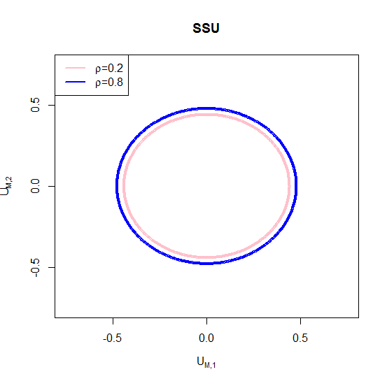
Figure 1: Comparison of theoretical $95\%$ acceptance regions of SSU test and of MANOVA for $K=2$ traits and $\rho=0.2,0.8$ (Compound Symmetry correlation). The area within the pink (blue) ellipse is the acceptance region when $\rho=0.2\>(0.8)$. Details of these plots are provided in LABEL:S-app2. SSU’s acceptance region is drawn using the marginal scores $U_{M,1}$ and $U_{M,2}$. MANOVA’s acceptance region is drawn based on the test $\boldsymbol{Z}^{\prime}\boldsymbol{I}(\boldsymbol{0})\boldsymbol{Z}$, where $\boldsymbol{I}(\boldsymbol{0})$ is Fisher Information matrix under $H_{0}:\boldsymbol{\beta}=\boldsymbol{0}$. The blue dotted line is the $\boldsymbol{1}$ vector and coincides with the major axes of the ellipses. When $\beta_{1}=\beta_{2}$, we expect $Z_{1}=Z_{2}$. The solid black square represents a situation where $\beta_{1}=\beta_{2}\gg 0$. When $\beta_{1}$ & $\beta_{2}$ are significantly apart, we expect the same for $Z_{1}$ & $Z_{2}$, and such a situation in represented by the dark green triangle.

The theoretical $95\%$ acceptance regions of SSU and MANOVA for $K=2$ correlated traits in Figure 1 provide a geometrical explanation of the above theorems. The acceptance region of SSU is drawn using the marginal scores $U_{M,1}$ and $U_{M,2}$. MANOVA’s acceptance region is drawn using the $2$ components $Z_{1}$ and $Z_{2}$ of vector $\boldsymbol{Z}$ since MANOVA is asymptotically equivalent to the test $\boldsymbol{Z}^{\prime}\boldsymbol{I}(\boldsymbol{0})\boldsymbol{Z}$. Here $\boldsymbol{Z}$ is an $N(\boldsymbol{0},\boldsymbol{I}(\boldsymbol{0})^{-1})$ variable and $\boldsymbol{I}(\boldsymbol{0})$ is Fisher Information matrix under $H_{0}:\boldsymbol{\beta}=\boldsymbol{0}$. Details of this equivalence and the acceptance region plots are provided in LABEL:S-app2. For SSU, a high true value of $\beta_{1}(\beta_{2})$ will be reflected by a high value of $U_{M,1}(U_{M,2})$. In Figure 1, observe that the SSU acceptance regions are almost circular in shape irrespective of correlation $\rho$. With increase in $\rho$, the shape of the acceptance region remains same. Only the size increases a little which causes slight loss in power to reject $H_{0}$. For MANOVA, a high true value of $\beta_{1}(\beta_{2})$ will be reflected by a high value of $Z_{1}(Z_{2})$. When $\rho\rightarrow 1$, notice that the acceptance region for MANOVA becomes elongated along the direction of $\boldsymbol{1}$ vector in Figure 1. Recall that for a CS correlation matrix, the eigen vector corresponding to the largest eigenvalue (for $\rho>0$) is along the direction of $\boldsymbol{1}$ vector. When the true genetic effect sizes are equal and in the same direction, the corresponding components of $\boldsymbol{Z}$ are equal as well and they will lie on vector $\boldsymbol{1}$. This suggests that the $Z$’s (and hence the non-zero genetic effects) need to be really large to cross the MANOVA acceptance region boundary for high $\rho$. The black box in Figure 1 represents such a situation, and it arises when the SNP is associated with both the correlated traits. This fail-to-reject situation will prevail even when the genetic effects are unequal but similar in magnitude. In genetic association studies, we may not expect equal effect sizes but we can expect them to be very close since each effect size is very small. On the other hand, if the effect sizes are very different, the $\boldsymbol{Z}$ vector will lie in some direction significantly away from the major axis $\boldsymbol{1}$ of the acceptance region. The closer it gets towards the minor axis, the greater is the chance for MANOVA statistic to fall outside the boundary and reject the null. The dark green triangle in Figure 1 represents a situation where MANOVA’s power to reject $H_{0}$ is higher when $\rho$ is higher. This is the situation when only one of the two traits is associated. Furthermore, Figure 1 shows that MANOVA’s loss in power will not be observed (irrespective of the strength and direction of within trait correlation) in studies where the effect sizes are reasonably large. This was observed in our simulation study with large genetic effects (simulation results not provided). It is also to be noted that if all the traits are associated but not all are correlated, MANOVA is not expected to lose power (refer section 3.4).

2.5 An alternative test: A unified score-based association test (USAT)

Our proposed test is motivated by the geometrical findings in section 2.4. As mentioned earlier, SSU test statistic does not explicitly incorporate within trait correlation and hence its acceptance region is not much affected when we increase the degree of dependency among the traits. On the other hand, MANOVA suffers from lack of power when the correlation is high and the genetic effect sizes are similar in magnitude and in same direction as the correlation. One, of course, does not know the true size and direction of the genetic effects and hence one would not know which association test to use. In such a scenario, one can see the clear advantage of combining MANOVA and SSU. We decided to choose the weight optimally from the data. We call our test unified score-based association test (USAT). The USAT test statistic is not exactly the best weighted combination of MANOVA and SSU. It is the minimum of the p-values of the different weighted combinations. Lee et al. (2012) proposed a similar test statistic based on minimum p-value in the context of rare variants in sequencing association studies.

Let $T_{M}$ be the MANOVA test statistic based on Wilk’s lambda. From Bartlett’s approximation, $T_{M}\overset{a}{\sim}\chi^{2}_{K}$. On the other hand, the SSU test statistic, denoted as $T_{S}$, has an approximate $a\chi^{2}_{d}+b$ distribution, where the parameters $a$ and $b$ and the degrees of freedom $d$ are estimated from the data using equation (3). Consider the weighted statistic $T_{\omega}=\omega T_{M}+(1-\omega)T_{S}$, where $\omega\in[0,1]$ is the weight. Both MANOVA and SSU are special cases of the class of statistics $T_{\omega}$. Under the null hypothesis of no association, for a given $\omega$, $T_{\omega}$ is approximately a linear combination of chi-squared distributions. For a given $\omega$, the p-value $p_{\omega}$ of the test statistic $T_{\omega}$ can be calculated using Liu et al. (2009) algorithm for chi-square approximation of non-negative quadratic forms. It is worth noting that the calculation of $p_{\omega}$ does not require independence assumption of the two test statistics (refer LABEL:S-app3).

Apriori the optimal weight $\omega$ is not known. We propose our optimal unified test USAT as

$$T_{USAT}=\min_{0\leq\omega\leq 1}p_{\omega}$$

For practical purposes, a grid of $11$ $\omega$ values were considered: $\{\omega_{1}=0,\omega_{2}=0.1,...,\omega_{10}=0.9,\omega_{11}=1\}$. A finer grid of more $\omega$ values did not change the USAT power curve much.

To find the p-value of our USAT test statistic, we need the null distribution of USAT. One option is to calculate the empirical p-value by considering several permuted datasets or by generating several datasets under the null (as done for Figure 4). Finding empirical p-values is computationally intensive and is not suitable when USAT is applied on a GWAS scale with large number of traits. We propose an approximate p-value calculation using a one-dimensional numerical integration. Observe that the p-value of statistic $T_{USAT}$ is

$$p_{USAT} = 1-P(T_{USAT}\leq t_{USAT})$$

$$= 1-P\left(T_{\omega_{1}}<q_{\min}(\omega_{1}),...,T_{\omega_{11}}<q_{\min}(\omega_{11})\right)\approx 1-\int F_{T_{S}}\big{(}\delta_{\omega}(x)|x\big{)}f_{T_{M}}(x)dx$$

where $t_{USAT}$ is the observed value of USAT test statistic for a given dataset, $q_{\min}(\omega_{b})$ is the $(1-t_{USAT})$-th percentile of the distribution of $T_{\omega_{b}}$ for a given $\omega=\omega_{b}$, $F_{T_{S}}(.)$ is the cdf of SSU test statistic $T_{S}$, $\delta_{\omega}(x)=\min_{\omega\in\{\omega_{1},...,\omega_{11}\}}\frac{q_{\min}(\omega)-\omega x}{1-\omega}$ and $f_{T_{M}}(.)$ is the pdf of MANOVA test statistic $T_{M}$. Mathematical details are provided in LABEL:S-app3.

3 Results

We compared the performances of different methods mentioned in sections 2.1, 2.2, 2.3. We investigated their type I errors and powers by simulating data on unrelated subjects under a variety of trait models. In Simulation 1 (section 3.1), we considered $K=2$ correlated traits with genetic effects in different directions and correlation $\rho$ varying between $-1$ and $1$. For Simulation 2 (section 3.2), we considered $K=5,10,20$ traits with genetic effects in the same direction as the positive correlation. CS correlation structure was considered. As part of Simulation 2, we also compared the performance of USAT against MANOVA and SSU. In Simulation 3 (section 3.3), we used data from Simulation 2 and investigated the type I error of USAT using the p-value approximation method described in section 2.5. In Simulation 4 (section 3.4), we used the same set-up as Simulation 2 to investigate the behaviors of existing methods under correlation structures other than CS.

For our simulation studies, we first simulated $X$ taking values $0,1,2$ with probabilities $(1-f)^{2},2f(1-f),f^{2}$ respectively. $f=0.2$ was the m.a.f. of the the single SNP. The two alleles at the SNP were sampled independently to ensure Hardy-Weinberg equilibrium. Conditional on $X$, we simulated $\boldsymbol{Y}$ for a fixed $K$ using the simulation model $\boldsymbol{Y}=\beta_{0}\boldsymbol{1}+\boldsymbol{\beta}X+\boldsymbol{\epsilon}$, where the vectors $\boldsymbol{Y}$, $\boldsymbol{1}$, $\boldsymbol{\beta}$, $\boldsymbol{\epsilon}$ are $K$-dimensional. We took $\beta_{0}=1$ and simulated $\boldsymbol{\epsilon}$ from $N_{K}(\boldsymbol{0},\sigma^{2}\boldsymbol{R}(\rho))$, where $\boldsymbol{R}(\rho)$ is a CS correlation matrix. The specific choices of $\boldsymbol{\beta}$, $\sigma^{2}$ and $\rho$ for each simulation are given in the sections 3.1 and 3.2. Before applying any method on the simulated datasets, we centered both $\boldsymbol{Y}$ and $\boldsymbol{X}$ for each dataset. We are interested in testing $H_{0}:\boldsymbol{\beta}=\boldsymbol{0}$. All the association tests except MultiPhen were coded by us in R 3.0.1 (R Development Core Team, 2014). For MultiPhen, we used ‘Joint Model’ output (p-value) from the R package MultiPhen 2.0.0.

3.1 Simulation 1: $K=2$ traits

We first studied the performances of different association tests by considering only $2$ correlated traits so that the genetic effects and the pairwise correlation can have different directions. We considered genetic effects $\boldsymbol{\beta}$ such that $0.2\%$ of the total variance of an associated trait was explained by the SNP. The total variance of an associated trait was taken to be $10$. This ensured that the variance due to SNP was $0.02$ while the residual variance was $\sigma^{2}=9.98$. For an unassociated trait, the variance explained by SNP was $0$ and hence its residual variance was same as the total variance. We considered 3 possible levels of association: no trait was associated ($\beta_{1}=0=\beta_{2}$), only the first trait was associated ($\beta_{1}=0.25,\beta_{2}=0$) and both the traits were associated ($\beta_{1}=0.25=\beta_{2}$). We also considered genetic effects in opposite directions ($\beta_{1}=0.25,\beta_{2}=-0.25$).

Table 1: Estimated type I errors of the afore mentioned existing association tests for $K=2$ correlated traits. $4$ values of pairwise correlation $\rho$ were considered. The p-values were calculated for $10,000$ null datasets with $4,000$ unrelated individuals. Type I error rate was calculated as the proportion of null datasets with p-value $\leq\alpha$.

$\alpha$	$\rho$	Fisher	minP	TATES	SSU	MANOVA	MultiPhen
$0.01$	$-0.8$	$0.029$	$0.009$	$0.012$	$0.010$	$0.009$	$0.010$
	$-0.2$	$0.012$	$0.011$	$0.011$	$0.011$	$0.011$	$0.011$
	$0.2$	$0.011$	$0.010$	$0.010$	$0.010$	$0.011$	$0.010$
	$0.8$	$0.026$	$0.008$	$0.012$	$0.009$	$0.009$	$0.009$
$0.05$	$-0.8$	$0.079$	$0.039$	$0.053$	$0.049$	$0.049$	$0.048$
	$-0.2$	$0.053$	$0.051$	$0.052$	$0.049$	$0.051$	$0.051$
	$0.2$	$0.051$	0.049	$0.051$	$0.05$	$0.052$	$0.05$
	$0.8$	$0.079$	$0.039$	$0.055$	$0.047$	$0.052$	$0.051$

First, type I error comparison was done for the 6 existing methods. For this purpose, we simulated $N=10,000$ null datasets with $n=4,000$ independent individuals. The type I error was calculated as the proportion of null datasets in which the p-value $\leq 0.01$ and $\leq 0.05$. Table 1 shows the type I errors for each of the methods for $4$ values of $\rho$: $-0.8,-0.2,0.2,0.8$. For high magnitude of correlation $\rho$, notice that Fisher’s method has inflated type I error while minP is conservative. Unlike minP, TATES is not conservative since it corrects for the relatedness among the traits. SSU maintains proper type I error since the distribution of the test statistic incorporates the within trait correlation structure. As expected, MANOVA and MultiPhen maintain correct type I error rate.

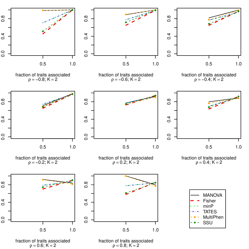
Figure 2: Empirical power curves of the different existing association tests for $K=2$ traits and different within trait correlation values $\rho=-0.8,-0.6,-0.4,-0.2,0.2,...,0.8$ based on $N=500$ datasets with $n=4,000$ unrelated subjects. Same direction and same size genetic effect used when both traits are associated (i.e., datasets are generated from an alternative model $H_{a2,1}:\beta_{1}=\beta_{2}>0$). Effect size of $0.25$ is used for the associated traits. The power is plotted along y-axis while the fraction of traits associated with the genetic variant is plotted along x-axis.

Next, we compared the powers of the methods. $N=500$ datasets with $n=4,000$ unrelated individuals were simulated for different levels of association. $8$ different values of correlation $\rho$ were used: $-0.8,-0.6,-0.4,-0.2,0.2,0.4,0.6,0.8$. Since the methods do not have comparable type I errors (as seen in Table 1), we plotted empirical power curves for comparison. The empirical power at $5\%$ error level was calculated in the following way. For each of Fisher’s method, MANOVA and SSU, the $95$-th quantile of the empirical distribution of the test statistic was determined based on the $N=500$ test statistics obtained from $N$ null datasets. Empirical power for these methods was calculated as the proportion of test statistics that exceeded the $95$-th quantile. For each of minP and TATES, the $5$-th quantile of the empirical distribution of the test statistic was determined using the $N=500$ test statistics under null. Empirical power was, then, calculated as the proportion of test statistics that could not exceed the $5$-th quantile. The empirical power of MultiPhen was determined using p-values in a way similar to empirical power calculation of minP and TATES. From Figure 2, we observe that, irrespective of the value of $\rho$, the tests that do not consider within trait correlation have increase in power with increase in the number of associated traits. They seem to have similar performance when both traits are associated. On the other hand, MANOVA and MultiPhen have similar performance and are usually the most powerful approaches for detecting association. But, both experience power loss when $\rho>0.5$ and both traits have same direction of association. For traits with genetic effects in opposite directions, similar behavior of MANOVA was observed (refer Figure LABEL:S-fig2 in LABEL:S-app9). The power of MANOVA drops when $\rho<-0.5$ and the 2 traits have opposite directions of association. These empirical observations on MANOVA are consistent with Corollary 2.3 of Theorem 2.2. No such power loss is observed for marginal model based approaches. In particular, SSU maintains correct type I error and does not experience power loss like MANOVA. This observation on SSU is consistent with our geometrical insight from Figure 1.

3.2 Simulation 2: $K=5,10,20$ traits

To further study the performance of different tests with increase in the number of correlated traits, we simulated three sets of data where the first set had $K=5$, second had $K=10$ and the third had $K=20$ correlated traits. We considered $N=500$ simulated datasets for each scenario with $n=400$ unrelated individuals. For this simulation study, we considered only non-negative genetic effects, and positive correlation $\rho=0.2,0.4,0.6$ between each pair of traits. The total variance of a trait was fixed at $10$. $\boldsymbol{\beta}$ was chosen such that $0.5\%$ of the total variance of an associated trait was explained by the single SNP. We considered 6 possible levels of association: $0\%$, $20\%$, $40\%$, $60\%$, $80\%$ or $100\%$ of the traits were associated with the SNP. Empirical power curves are presented for comparison.

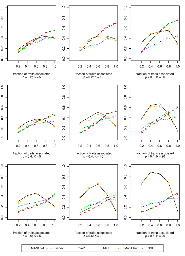
Figure 3: Empirical power curves of the different existing association tests for $K=5,10,20$ traits and different within trait correlation values $\rho=0.2,...,0.6$ based on $N=500$ datasets with $n=400$ unrelated subjects. Same effect size of $0.395$ is used for all the associated traits. The power is plotted along y-axis while the fraction of traits associated with the genetic variant is plotted along x-axis.

From Figure 3, we again observe how MANOVA suffers from power loss at ‘complete association’ when the within trait correlation is high. This power loss increases with increase in total number of correlated traits. At ‘complete association’ (where MANOVA loses power), the power difference between MANOVA and other methods (such as SSU) increases with increase in number of correlated traits and decrease in correlation $\rho$. At a given ‘partial association’, MANOVA is seen to dominate over other methods. Here, the difference in powers of MANOVA and any other method increases with increase in number of traits as well as the correlation. MANOVA’s performance in this experiment is consistent with the asymptotic result in Theorem 2.1.

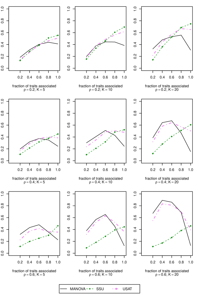
Figure 4: Empirical power curves of the SSU and MANOVA tests along with our novel approach USAT (based on an optimal combination of SSU and MANOVA). $K=5,10,20$ traits have been simulated at different within trait correlation values $\rho=0.2,0.4,0.6$. For each value of $K$ and $\rho$, there were $N=500$ datasets of $n=400$ unrelated individuals. Same effect size of $0.395$ was used for the traits that are associated. The power is plotted along y-axis while the fraction of traits associated with the genetic variant is plotted along x-axis.

Next we studied the performance of our approach USAT compared to MANOVA and SSU. We plotted empirical power curves in Figure 4 for comparison. Empirical powers for MANOVA and SSU were calculated as in section 3.1. Empirical power calculation of USAT was implemented in a way similar to minP and TATES (as described in section 3.1). Observe that USAT has better power than MANOVA whenever it suffers from power loss due to same direction of residual correlation and equal-sized genetic effects. In such situations, SSU performs significantly better than MANOVA, and USAT follows the SSU power curve closely. In other situations where MANOVA is seen to be most powerful among existing methods, USAT tends to have power close to MANOVA. USAT maximizes power by adaptively using the data to combine the MANOVA and the SSU approach.

3.3 Simulation 3: p-value approximation for USAT

In this section, we applied our approximate p-value approach for finding USAT p-values (discussed in section 2.5) to study its impact on type I error. We generated $N=100,000$ independent datasets (as in section 3.2) with $n=10,000$ unrelated individuals under $H_{0}$. The type I error was estimated by the proportion of datasets in which the asymptotic approximate p-value of USAT test statistic was $\leq 10^{-4}$, $\leq 10^{-3}$, $\leq 10^{-2}$, and $\leq 0.05$. Table 2 gives the estimated type I error rates for USAT using p-value approximation. The estimated values of type I error for different values of $K$ and $\rho$ were very close to the true error level $\alpha$.

Table 2: Estimated type I errors of the approximate p-value calculation approach for our USAT test. The p-values were calculated for $100,000$ null datasets with $10,000$ unrelated individuals. Type I error rate was calculated as the proportion of datasets that had approximate p-value $\leq\alpha$.

K		5			10			20
$\rho$	0.2	0.4	0.6	0.2	0.4	0.6	0.2	0.4	0.6
$\alpha=10^{-4}$	$0.00008$	$10^{-4}$	$0.00008$	$0.00015$	$10^{-4}$	$0.00008$	$0.00015$	$0.00011$	$10^{-4}$
$\alpha=10^{-3}$	$0.00081$	$0.00092$	$0.00086$	$0.00108$	$0.00099$	$0.00089$	$0.00149$	$0.00117$	$0.00109$
$\alpha=10^{-2}$	$0.0082$	$0.0091$	$0.0093$	$0.0094$	$0.0098$	$0.0097$	$0.0103$	$0.0104$	$0.0103$
$\alpha=0.05$	$0.0362$	$0.0413$	$0.0438$	$0.0397$	$0.0441$	$0.0461$	$0.0431$	$0.0463$	$0.0471$

3.4 Simulation 4: Other correlation structures

We first considered an independent structure. Apart from the residual correlation matrix $\boldsymbol{R}(\rho)$, the data simulation was exactly same as in Simulation 2 (section 3.2). The figures and detailed explanations can be found in LABEL:S-app4. When all the traits are independent (i.e., $\boldsymbol{R}(\rho)=\boldsymbol{I}_{K}$), MANOVA does not suffer from power loss at any level of association. Empirical power curves (Figure LABEL:S-fig4i) showed that the performances of all the methods described in sections 2.1, 2.2, 2.3, except minP and TATES, were similar. As expected, the powers steadily increased with increase in number of associated traits. Next we considered a correlation structure where the first $80\%$ of the traits had pairwise correlation $\rho$ while the rest were independent. Empirical power curves (Figure LABEL:S-fig4ii) showed that MANOVA suffered power loss when only the correlated traits were associated. Performance of MANOVA improved when the SNP was associated with some of the uncorrelated traits. This simulation study showed us that MANOVA may not experience power loss even when all the traits are associated if some of them are uncorrelated. LABEL:S-app5 provides a theoretical support for this observation. The third type of non-CS correlation structure that we considered was AR$1(\rho)$ (Figure LABEL:S-fig4iii). MANOVA’s power loss was mainly observed for small $K$ and strong $\rho$. With increase in $K$ and decrease in $\rho$, MANOVA did not experience power loss even at ‘complete association’. The strength of AR$1(\rho)$ correlation becomes negligible at or near ‘complete association’ when $\rho$ is small and $K$ is moderately large. For all these trait models, the power curves of marginal model based approaches rose with increase in number of associated traits (irrespective of strength or direction of residual correlation). All these observations on MANOVA for various correlation structures were expected based on our geometrical insight from Figure 1 (section 2.4).

3.5 Real Data Analysis

The ARIC study is an ongoing prospective study designed to investigate the etiology and natural history of atherosclerosis and its clinical manifestations, and to measure variation in cardiovascular risk factors, medical care and disease by race, gender, place and time (The ARIC Investigators, 1989). ARIC has collected measures on many T2D-related traits at 4 separate visits over a 9-year period. For our analysis, we focused on the Caucasian participants and the following 3 T2D related quantitative traits measured at visit $4$ ($1996-98$): fasting glucose; 2-hour glucose from an oral glucose tolerance test; fasting insulin. The pairwise correlations among these 3 traits were within $(0.2,0.35)$. As in most studies of T2D, BMI was used as a covariate. Individuals with diagnosed or treated diabetes at visit $4$ and individuals with missing traits were excluded, leaving $5,816$ in our analytic sample. More details on the phenotypes and the choice of covariates can be found in LABEL:S-app6.

The ARIC cohort has been genotyped using the Affymetrix Genome-Wide SNP Array 6.0. Genotyping was completed at the Broad Institute of MIT and Harvard in three batches; the Birdseed algorithm was used for genotype calling. Imputation was performed using Mach $1.0$ $86$ and HapMap release 21 (Build 35). SNPs with a call rate $<90\%$, m.a.f. $<1\%$, or deviation from Hardy-Weinberg equilibrium ($p<10^{-6}$) were excluded for imputation. There was a total of $2.5$ million genotyped or imputed SNPs. Apart from USAT and MANOVA, we also performed separate univariate analyses to emphasize the importance of joint analysis over univariate ones. Before implementing any of these approaches, we centered both phenotype and genotype data. SNPs with m.a.f. $<1\%$ were excluded. All statistical models were adjusted for Age, Sex and BMI.

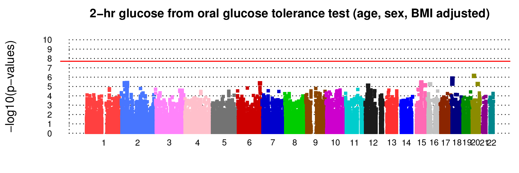
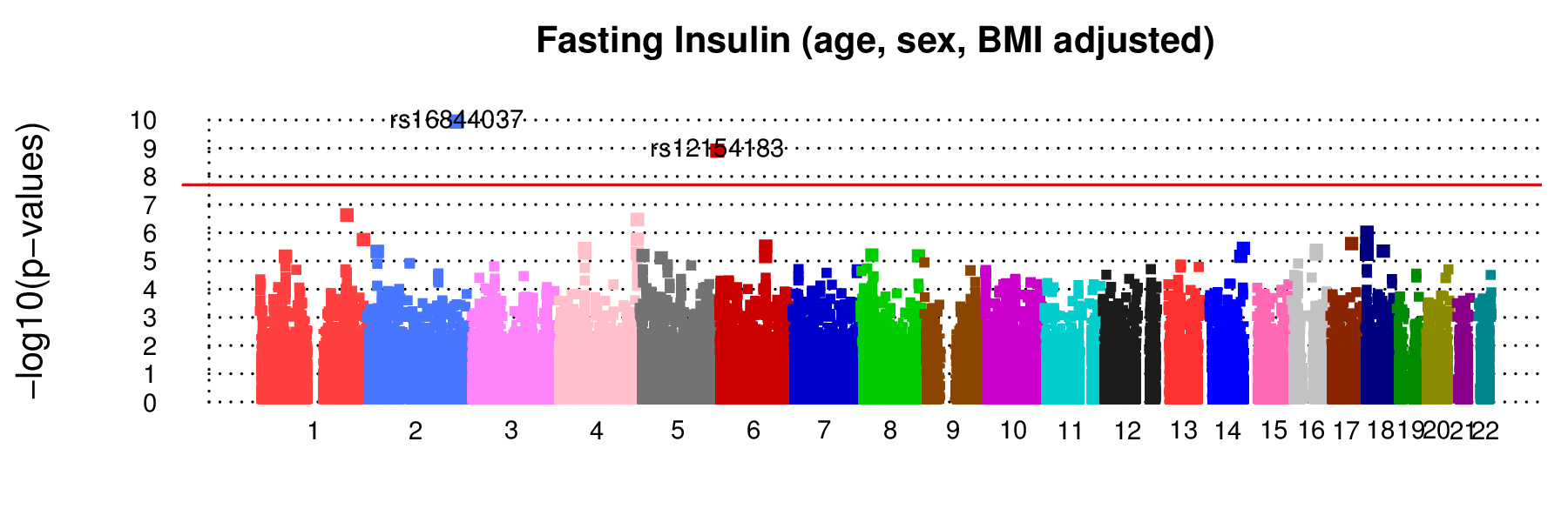
Figure 5: ARIC Study: Manhattan plots of negative log-transformed p-values of the univariate analyses are plotted against base pair positions for chromosomes $1-22$. Age, Sex and BMI were adjusted in the statistical models. The red horizontal line in each plot corresponds to significance level $0.05$ after Bonferroni correction for $2.5\times 10^{6}$ SNPs. $53$ SNPs (all from chr 2) detected as significant for fasting glucose; $2$ such SNPs (from chr 2 and 6) for fasting insulin; and none for the other trait. Note that many of these significant SNPs are in high linkage disequilibrium.

Figure 5 shows the manhattan plots of negative log-transformed p-values for the single trait single SNP analyses for chromosomes $1-22$. The red horizontal line (at $7.7$) in each plot indicates the log-transformed GWAS significance p-value $2\times 10^{-8}$. There were $53$ and $2$ significant SNPs respectively for fasting glucose and fasting insulin. On the other hand, there were $86$ and $75$ signals for MANOVA and USAT respectively that reached this stringent Bonferroni corrected threshold (refer Figure 6, and Table LABEL:S-t:sigall in LABEL:S-app8). Most of these signals mapped near the genes GCKR, ABCB11, C2orf16, CCDC121, ZNF512, FAM148A, C2CD4A, which are already known to be associated with diabetes related traits (Yamauchi et al., 2010; Kraja et al., 2011, for example). It is worth noting that these detected SNPs are in high linkage disequilibrium (LD). Among the SNPs reported in Table LABEL:S-t:sigall, MANOVA and USAT respectively detected $36$ and $26$ SNPs that none of the univariate analyses could detect. Most notable genes that the univariate analyses completely missed are GCKR (on chr $2$) and FAM148A (on chr $15$).

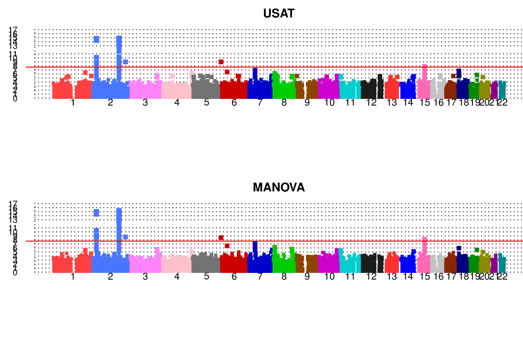
Figure 6: ARIC Study: Manhattan plots of negative log-transformed p-values of multivariate analyses (USAT and MANOVA) are plotted against base pair positions for chromosomes $1-22$. Age, Sex and BMI were adjusted in the statistical models. The red horizontal line in each plot corresponds to significance level $0.05$ after Bonferroni correction for $2.5\times 10^{6}$ SNPs. Note that many of these significant SNPs are in high linkage disequilibrium.

Since most of the detected SNPs in Figure 6 are in high LD, Table 3 reports only the important SNPs after removing the ones in high LD. In a group of highly correlated SNPs (i.e., SNPs with estimated absolute pairwise correlation coefficient $>0.8$ with another SNP), we kept one SNP as a representative. The choice of representative SNP was based on previous reports of association. The correlation coefficients (as measures of LD) were obtained from PLINK (Purcell et al., 2007) using the command plink --file mydata --r. The minor allele T of rs1260326 (gene GCKR of chr $2$) is known to be associated with T2D and hypertriglyceridemia. Risk allele A of rs13022873 (gene ZNF512 of chr $2$) was found to be significantly associated with waist circumference (a T2D related trait highly correlated with BMI) and triglycerides (Kraja et al., 2011). rs13431652 (gene G6PC2 of chr $2$) was reported to be a potentially causative SNP linking G6PC2 to increased fasting plasma glucose levels and elevated promoter activity (Bouatia-Naji et al., 2010). The rs1402837 T allele (gene G6PC2 of chr $2$) is known to be associated with blood sugar levels (glycated hemoglobin levels). McCaffery et al. (2013) reported that SNPs in ABCB11 (like rs484066) of chr $2$ are associated with weight loss and regain. Meta-analysis of several GWAS found rs17271305 (gene VPS13C of chr $15$) to be associated with glucose levels 2 hours after an oral glucose challenge (Saxena et al., 2010). The diabetogenic A allele of rs7172432 (gene VPS13C/C2CD4A/C2CD4B of chr $15$) significantly impairs glucose-stimulated insulin response in non-diabetics (Grarup et al., 2011). The remaining signals in Table 3 have not been previously reported.

Table 3: List of SNPs that exceed the significance level of $0.05$ after Bonferroni correction for the number of SNPs (i.e., p-value threshold $2\times 10^{-8}$) for USAT and MANOVA. The SNPs listed here are the ones left after LD screening. In a group of highly correlated SNPs (i.e., SNPs with estimated absolute pairwise correlation coefficient $>0.8$ with another SNP), one SNP was kept as a representative. $p$ values for the univariate analysis of the individual traits are also provided for these significant SNPs. SNP rs ID in bold is the one detected solely by MANOVA but not by USAT at this stringent genome-wide significance level. The abbreviations used are FG (Fasting Glucose), 2-hr GL (2-hour glucose from an oral glucose tolerance test), FI (Fasting Insulin).

			MANOVA	USAT	Univariate Analysis $p$
chr	SNP	position	$p$	$p$	FG	2-hr GL	FI
$2$	$rs1260326$	$27584444$	$3.77\times 10^{-15}$	$4.44\times 10^{-15}$	$1.24\times 10^{-4}$	$6.26\times 10^{-6}$	$1.24\times 10^{-5}$
$2$	$rs13022873$	$27669014$	$9.94\times 10^{-10}$	$2.34\times 10^{-9}$	$1.49\times 10^{-2}$	$6.01\times 10^{-6}$	$1.07\times 10^{-2}$
$2$	$rs13431652$	$169461661$	$1.85\times 10^{-13}$	$5.48\times 10^{-13}$	$2.24\times 10^{-12}$	$9.57\times 10^{-1}$	$2.85\times 10^{-1}$
$2$	$rs1402837$	$169465600$	$4.91\times 10^{-9}$	$1.15\times 10^{-8}$	$2.78\times 10^{-10}$	$5.18\times 10^{-2}$	$8.07\times 10^{-1}$
$2$	$rs484066$	$169490727$	$2.01\times 10^{-12}$	$2.32\times 10^{-12}$	$6.10\times 10^{-12}$	$8.54\times 10^{-1}$	$4.87\times 10^{-1}$
$2$	$rs16844037$	$210561151$	$1.92\times 10^{-9}$	$1.04\times 10^{-9}$	$2.16\times 10^{-1}$	$2.56\times 10^{-2}$	$1.14\times 10^{-10}$
$6$	$rs12154183$	$295724$	$2.81\times 10^{-9}$	$1.02\times 10^{-9}$	$4.01\times 10^{-1}$	$9.55\times 10^{-1}$	$1.21\times 10^{-9}$
$15$	$rs17271305$	$60120272$	$6.87\times 10^{-9}$	$1.35\times 10^{-8}$	$6.29\times 10^{-3}$	$1.17\times 10^{-5}$	$2.86\times 10^{-1}$
$15$	$\boldsymbol{rs7172432}$	$60183681$	$1.68\times 10^{-8}$	$5.98\times 10^{-8}$	$7.98\times 10^{-4}$	$3.52\times 10^{-4}$	$4.88\times 10^{-2}$

In Table 3, we notice one SNP (rs7172432) that USAT missed at the stringent significance level of $2\times 10^{-8}$. One also notices that difference in the p-values of USAT and MANOVA for this SNP is negligible. If one takes a closer look at the manhattan plots of Figure 6, one will find that certain SNPs are prominently visible for USAT but not for MANOVA (even though none could reach genome wide significance). The most noticeable regions are in chr $1$ (rs4427409 and rs17434403 with USAT $p$ $4.95\times 10^{-7}$ and $4.86\times 10^{-7}$), chr $4$ (rs4861722 and rs11729070 with USAT $p$ $5.76\times 10^{-7}$ and $3.86\times 10^{-7}$) and in chr $18$ (rs17497377 and rs2864527 with USAT $p$ $1.73\times 10^{-7}$ and $7.59\times 10^{-7}$). None of these signals have been previously reported.

4 Discussion

In the study of a complex disease, several correlated traits are often measured as risk factors for the disease. There may be genetic variants affecting several of these traits. Analyzing multiple disease-related traits could potentially increase power to detect association of genetic variants with such a disease. The elucidation of genetic risk factors of such diseases will help us in better understanding and developing therapeutics against them. In this paper, we have studied some of the common univariate and multivariate approaches for analyzing association between multiple phenotypes and a genetic variant. Our simulation results showed that no single method perform uniformly better than the others under the simulation scenarios we considered. Multivariate methods like MANOVA and MultiPhen usually had higher power than the univariate tests only in situations where a few of the correlated traits were associated. Univariate model based methods in sections 2.1 & 2.2 outperformed multivariate methods when all the correlated traits were associated and the genetic effects as well as the residual correlations were in the same direction. Under the assumption of a CS residual correlation structure, we established theoretical conditions as to when MANOVA would start losing power. Although we have not established similar theoretical conditions for other correlation structures, we have seen similar behavior of MANOVA in our simulation studies.

We also proposed a novel weighted approach USAT, which maximizes power by adaptively using the data to optimally combine MANOVA and the SSU test. Approximate USAT p-values can be computed using a very fast one-dimensional numerical integration, which makes implementation on GWAS data easy. As shown by our simulation studies, USAT maintains correct Type I error (refer Table 2) and has good power in detecting association (refer Figure 4). Unlike MANOVA, USAT is powerful in detecting pleiotropy under the simulation models we considered. The ARIC data analysis not only emphasized the importance of joint analysis of correlated endo-phenotypes over univariate analyses but also showed the power of USAT in detecting SNPs that might have influence on T2D risk. As in the real data analysis, adjustment of other covariates can be easily done for USAT (details in LABEL:S-app7).

Finally, the simulation scenarios we considered are not exhaustive. Under the scenarios we considered, we found it best to combine the SSU and the MANOVA tests. The relative behavior of these two tests did not vary much with change in m.a.f. (refer Figure LABEL:S-fig4-maf5 in LABEL:S-app10), or with increase in the number of correlated traits. Our simulation studies also assumed no missing data and no trait outliers. USAT requires complete phenotype data. In presence of missing traits, one may consider imputation before performing association analysis. van der Sluis et al. (2013) showed that $10\%$ missing-completely-at-random data caused quite a drop in power for MANOVA when only 1 trait was associated. O’Reilly et al. (2012) showed that in the presence of outliers in the phenotype distribution, MANOVA and the standard univariate approach were substantially inflated for low m.a.f. We simulated data for an additive model only and did not consider any non-additive genetic model and/or interactions. In future, we intend to study how power of our USAT test would be affected in such situations.

Supporting Information

Appendices S1$-$S10 are available with this paper at the end.

References

- Aschard et al. (2014) Aschard, H., Vilhjálmsson, B., Greliche, N., Morange, P.-E., Trégouët, D.-A., and Kraft, P. (2014). Maximizing the power of principal-component analysis of correlated phenotypes in genome-wide association studies. Am J Hum Genet 94, 662–676.
- Basu et al. (2013) Basu, S., Zhang, Y., Ray, D., Miller, M., Iacono, W., and McGue, M. (2013). A rapid gene-based genome-wide association test with multivariate traits. Hum Hered 76(2), 53–63.
- Blair et al. (2013) Blair, D., Lyttle, C., Mortensen, J., et al. (2013). A nondegenerate code of deleterious variants in mendelian loci contributes to complex disease risk. Cell 155, 70–80.
- Bouatia-Naji et al. (2010) Bouatia-Naji, N., Bonnefond, A., Baerenwald, D. A., et al. (2010). Genetic and functional assessment of the role of the rs13431652-A and rs573225-A alleles in the G6PC2 promoter that are strongly associated with elevated fasting glucose levels. Diabetes 59(10), 2662–71.
- Ferreira and Purcell (2009) Ferreira, M. and Purcell, S. (2009). A multivariate test of association. Bioinformatics 25, 132–133.
- Fisher (1925) Fisher, R. (1925). Statistical Methods for Research Workers. Oliver and Boyd, Edinburgh.
- Galesloot et al. (2014) Galesloot, T., van Steen K., Kiemeney, L., Janss, L., and Vermeulen, S. (2014). A comparison of multivariate genome-wide association methods. PLoS One 9(4), e95923.
- Germain et al. (2011) Germain, M., Saut, N., Greliche, N., Dina, C., et al. (2011). Genetics of venous thrombosis: Insights from a new genome wide association study. PLoS One 6, 9.
- Grarup et al. (2011) Grarup, N., Overvad, M., Sparsø, T., Witte, D., et al. (2011). The diabetogenic VPS13C/C2CD4A/C2CD4B rs7172432 variant impairs glucose-stimulated insulin response in 5,722 non-diabetic Danish individuals. Diabetologia 54(4), 789–94.
- Korte et al. (2012) Korte, A., Vilhjálmsson, B., Segura, V., Platt, A., Long, Q., and Nordborg, M. (2012). A mixed-model approach for genome-wide association studies of correlated traits in structured populations. Nat Genet 44, 1066–1071.
- Kraja et al. (2011) Kraja, A., Vaidya, D., Pankow, J., Goodarzi, M., et al. (2011). A bivariate genome-wide approach to metabolic syndrome: STAMPEED consortium. Diabetes 60(4), 1329–39.
- Lee et al. (2012) Lee, S., Wu, M., and Lin, X. (2012). Optimal tests for rare variant effects in sequencing association studies. Biostatistics 13, 762–775.
- Liu et al. (2009) Liu, H., Tang, Y., and Zhang, H. (2009). A new chi-square approximation to the distribution of non-negative definite quadratic forms in non-central normal variables. Comput Stat Data Anal 53, 853–856.
- Maity et al. (2012) Maity, A., Sullivan, P., and Tzeng, J. (2012). Multivariate phenotype association analysis by marker-set kernel machine regression. Genet Epidemiol 36(7), 686–695.
- McCaffery et al. (2013) McCaffery, J., Papandonatos, G., Huggins, G., et al. (2013). Human cardiovascular disease IBC chip-wide association with weight loss and weight regain in the look AHEAD trial. Hum Hered 75(2-4), 160–74.
- Muller and Peterson (1984) Muller, K. and Peterson, B. (1984). Practical methods for computing power in testing the multivariate general linear hypothesis. Comput Stat Data Anal 2(2), 143–158.
- O’Reilly et al. (2012) O’Reilly, P., Hoggart, C., Pomyen, Y., Calboli, C., et al. (2012). Multiphen: Joint model of multiple phenotypes can increase discovery in gwas. PLoS One 7(5), e34861.
- Pan (2009) Pan, W. (2009). Asymptotic tests of association with multiple SNPs in linkage disequilibrium. Genet Epidemiol 33, 497–507.
- Purcell et al. (2007) Purcell, S., Neale, B., Todd-Brown, K., et al. (2007). PLINK: a tool set for whole-genome association and population-based linkage analyses. Am J Hum Genet 81, 559–575.
- R Development Core Team (2014) R Development Core Team (2014). R: A Language and Environment for Statistical Computing. R Foundation for Statistical Computing, Vienna, Austria.
- Ried et al. (2014) Ried, J., Shin, S.-Y., Krumsiek, J., et al. (2014). Novel genetic associations with serum level metabolites identified by phenotype set enrichment analyses. Hum Mol Genet .
- Saxena et al. (2010) Saxena, R., Hivert, M., Langenberg, C., et al. (2010). Genetic variation in GIPR influences the glucose and insulin responses to an oral glucose challenge. Nat Genet 42(2), 142–8.
- Souto et al. (2000) Souto, J., Almasy, L., Borrell, M., Blanco-Vaca, F., and Mateo, J. (2000). Genetic susceptibility to thrombosis and its relationship to physiological risk factors: The GAIT study. genetic analysis of idiopathic thrombophilia. Am J Hum Genet 67(6), 1452–1459.
- Stephens (2013) Stephens, M. (2013). A unified framework for association analysis with multiple related phenotypes. PLoS One 8 (7), e65245.
- Tang and Ferreira (2012) Tang, C. and Ferreira, M. (2012). A gene-based test of association using canonical correlation analysis. Bioinformatics 28(6), 845–850.
- The ARIC Investigators (1989) The ARIC Investigators (1989). The Atherosclerosis Risk in Communities (ARIC) Study: design and objectives. Am J Epidemiol 129(4), 687–702.
- van der Sluis et al. (2013) van der Sluis, S., Posthuma, D., and Dolan, C. (2013). TATES: efficient multivariate genotype-phenotype analysis for genome-wide association studies. PLoS Genet 9(1), e1003235.
- Yamauchi et al. (2010) Yamauchi, T., Hara, K., Maeda, S., Yasuda, K., et al. (2010). A genome-wide association study in the japanese population identifies susceptibility loci for type 2 diabetes at UBE2E2 and C2CD4A-C2CD4B. Nat Genet 42(10), 864–868.
- Yang et al. (2011) Yang, J., Lee, H., Goddard, M., and Visscher, P. (2011). GCTA: A tool for Genome-wide Complex Trait Analysis. Am J Hum Genet 88(1), 76–82.
- Yang and Wang (2012) Yang, Q. and Wang, Y. (2012). Review article: Methods for analyzing multivariate phenotypes in genetic association studies. J Probab Stat 2012, 13.
- Zhang (2005) Zhang, J.-T. (2005). Approximate and asymptotic distributions of chi-squared-type mixtures with applications. J Am Stat Assoc 100, 273–285.
- Zhang et al. (2009) Zhang, L., Pei, Y., Li, J., Papasian, C., and Deng, H. (2009). Univariate/multivariate genome-wide association scans using data from families and unrelated samples. PLoS One 4, e6502.
- Zhou and Stephens (2012) Zhou, X. and Stephens, M. (2012). Genome-wide efficient mixed model analysis for association studies. Nat Genet 44(7), 821–824.
- Zhou and Stephens (2014) Zhou, X. and Stephens, M. (2014). Efficient multivariate linear mixed model algorithms for genome-wide association studies. Nat Methods 11, 407–409.