Hyperbolic Metamaterials with Bragg Polaritons

Abstract

We propose a novel mechanism for designing quantum hyperbolic metamaterials with use of semiconductor Bragg mirrors containing periodically arranged quantum wells. The hyperbolic dispersion of exciton-polariton modes is realized near the top of the first allowed photonic miniband in such structure which leads to formation of exciton-polariton X-waves. Exciton-light coupling provides a resonant non-linearity which leads to non-trivial topologic solutions. We predict formation of low amplitude spatially localized oscillatory structures: oscillons described by kink shaped solutions of the effective Ginzburg-Landau-Higgs equation. The oscillons have direct analogies in the gravitational theory. We discuss implementation of exciton-polariton Higgs fields for the Schrödinger cat state generation.

Introduction A remarkable similarity between propagation of electromagnetic waves in inhomogeneous media described by the Maxwell’s equations and propagation of photons in curved space-time described by the general relativity laws offers a possibility of designing media where light propagates along pre-defined curved trajectories. This concept, known as transformation optics NatureMaterials93872010 not only allowed emulating many gravitational effects such as gravitational lensing NatPhoton79022013 , event horizon ProgressinOptics53692009 etc, but also led to a bunch of intriguing practical applications, such as optical cloaking ContemporaryPhysics542732013 , and superresolution optical imaging PRL8539662000 . Construction of the media with predefined profiles of electric and magnetic permeabilities is feasible with use of metamaterials IEEETrans4720751999 , artificial periodic structures whose optical properties are governed both by the electromagnetic response of individual structure elements and by the geometry of the lattice. Hyperbolic metamatrials (HMM’s) are highly anisotropic media that have hyperbolic (or indefinite) dispersion NatPhoton79582013 , determined by their effective electric and/or magnetic tensors. Such structures represent the ultra-anisotropic limit of traditional uniaxial crystals. One of the diagonal components of either permittivity ($\varepsilon$) or permeability ($\mu$) tensors of HMM has an opposite sign with respect to the other two diagonal components.

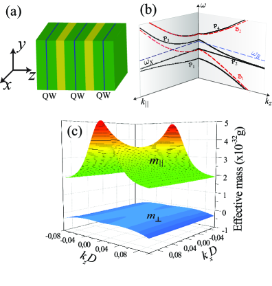
Figure 1: (a) – Schematic picture of spatially periodical structure (“Bragg mirror”), (b) – dispersion characteristics for four Bragg exciton-polariton branches (black solid lines); photonic Bragg mode dispersion is shown with red dashed lines, and, (c) is the effective mass dispersion for the lower polariton branch $\mathcal{P}_{1}$.

Recently, HMMs have attracted an enhanced attention both due to the promising applications in quantum lifetime engineering ApplPhysB1002152010 and subwavelength image transfer Science31516862007 , and because of their relatively low production costs as compared to other optical metamaterial designs. In contrast to all-dielectric uni-axial anisotropic media for which both dielectric permittivities are positive: $\varepsilon_{1}\equiv\varepsilon_{x}=\varepsilon_{y}>0$ and $\varepsilon_{2}\equiv\varepsilon_{z}>0$, in HMMs $\varepsilon_{1}$ and $\varepsilon_{2}$ have opposite signs in some frequency range due to the presence of metallic layers. As a result, the analogy between wave propagation governed by the Helmholtz equation and the effective Klein-Gordon equation for massive particle with fictitious time coordinate can be obtained for the description of a coherent CW laser beam propagation in such a structure. This analogy makes possible creation of the Minkowski space-time using HMMs PRA880338432013 . Applications of HMMs for modelling gravity and cosmology problems within scalar $\phi^{4}$-field theories require introducing a strong Kerr-like nonlinearity to the medium,  RubakovClassicalTheoryofGaugeFields2002 . However, the nonlinear response of the conventional HMMs is relatively weak. Moreover, most of the studied HMMs are essentially periodic arrays of metallic inclusions, characterised by large ohmic losses and decay of the electromagnetic field propagation.

To overcome these problems, in this Letter we propose a novel approach for emulating quantum effects in curved space-time using resonant semiconductor Bragg mirrors. Light propagation in such structures has been extensively studied both in theory and in experiments FizTverdTela3621181994 ; JApplPhys795951996 ; PRA640138092001 ; PRB80121306R2009 ; KavokinBaumbergMicrocavities2007 ; PRL1060764012011 . In particular, the dramatic modulation of the reflectivity spectra of Bragg spectra in the vicinity of exciton resonances has been predicted in JApplPhys795951996 . The peculiar dispersion of mixed photon-exciton modes in Bragg arranged quantum wells (QWs) has been discussed in literature (see, e.g. PRA640138092001 ; PRB80121306R2009 ; KavokinBaumbergMicrocavities2007 ; PRL1060764012011 ). Here we show that planar periodic semiconductor Bragg mirror structures with embedded QWs allow for controlling the signs of effective masses of mixed light-matter quasiparticles termed Bragg exciton-polaritons in order to create a quantum HMM. Exciton-polaritons are responsible for the strong nonlinear dielectric susceptibility of the system due to their excitonic part, while their dispersion properties can be tailored through the photonic part by tuning the layer thicknesses PRB80121306R2009 . The magnitude and sign of the polariton effective mass in such structures affect the effective dielectric permeabilities which are crucial for designing HMMs, cf. PRA890636242014 .

Bragg mirror model. The semiconductor structure that we are discussing here is schematically shown in Fig. 1(a). It consists of the periodic array of alternating dielectric layers with QWs placed in the centres of the layers of one type. The exciton frequency is tuned to the high frequency edge of the second photonic band gap, which is characterized by the saddle point in the dispersion surface, cf. PRB80121306R2009 . The Hamiltonian of the structure in Fig. 1 has a generic structure, that is $\hat{H}=\hat{H}_{\mathrm{ph}}+\hat{H}_{X}+\hat{H}_{\mathrm{coup}}+\hat{H}_{\mathrm{nl}}$ where $\hat{H}_{\mathrm{ph}}$ is the photonic part, $\hat{H}_{X}$ is the excitonic part, $\hat{H}_{\mathrm{coup}}$ accounts for the exciton-photon coupling, and $\hat{H}_{\mathrm{nl}}$ is the nonlinear part, originated from the exciton-exciton scattering. If we consider the frequencies in the vicinity of the second photonic band gap of the Bragg mirror, we can diagonalize the linear part of the Hamiltonian $\hat{H}$, using the approach described in PRA640138092001 to obtain the dispersions of the four polariton branches $\mathcal{P}_{1}$, $\mathcal{P}_{2}$, $\mathcal{P}_{3}$, $\mathcal{P}_{4}$, which are shown in Fig. 1(b); for more details see the supplemental material SuM .

The lower branch (LB) of polaritons is characterized by the effective mass tensor whose diagonal components differ in sign. In general the effective mass tensor is dispersive due to the non-parabolicity of the polariton band, however for the wave vectors small compared to the inverse period of the structure $1/D$, one can safely assume the tensor components constant (see Fig. 1(c)). Note that due to the smallness of the effective mass, exciton polaritons remain within the light cone, i. e. at the wave vectors smaller than $1/D$, even at room temperature.

In general case, the Hamiltonian $\hat{H}$ for the structure in Fig. 1 in the polariton basis is given by

$$\hat{H}=\displaystyle\sum_{i}\displaystyle\sum_{\mathbf{q}}\hbar\omega_{i}(\mathbf{q})\hat{c}_{i}^{\dagger}(\mathbf{q})\hat{c}_{i}(\mathbf{q})+\frac{g_{0}}{2}\displaystyle\sum_{\begin{subarray}{c}i,j\\ k,l\end{subarray}}\displaystyle\sum_{\begin{subarray}{c}\mathbf{q}_{1},\mathbf{q}_{2}\\ \mathbf{q}\end{subarray}}\mathrm{X}_{{i}}(\mathbf{q}_{1}+\mathbf{q})\mathrm{X}_{{j}}(\mathbf{q}_{2}-\mathbf{q})\mathrm{X}_{{k}}(\mathbf{q}_{1})\mathrm{X}_{{l}}(\mathbf{q}_{2})\hat{c}_{i}^{\dagger}(\mathbf{q}_{1}+\mathbf{q})\hat{c}_{j}^{\dagger}(\mathbf{q}_{2}-\mathbf{q})\hat{c}_{k}(\mathbf{q}_{1})\hat{c}_{l}(\mathbf{q}_{2}),$$ (1)

where $i,j,k,l=\left\{1,2,3,4\right\}$ enumerate polariton branches with corresponding frequencies $\omega_{i}$; $\mathbf{q}$ is an exciton-polariton wave-vector, $\hat{c},\hat{c}^{\dagger}$ are the annihilation and creation operators, $\mathrm{X}_{i,j,k,l}$ are the Hopfield coefficients defining the exciton fraction in the polariton state. The nonlinear coupling constant can be approximated by $g_{0}\approx\left.6E_{b}{a_{b}^{3}D}\right/{d_{\rm QW}V}$, where $E_{b}$ is the exciton binding energy, $a_{b}$ is the exciton Bohr radius, $D$ is period of the structure, $d_{\rm QW}$ is the QW width, and $V$ is the QW area. Hereafter we restrict ourselves only to LB neglecting the inter-branch scattering processes. In real space, we will describe LB polaritons by the field operator $\hat{\Psi}$ defined as

$$\hat{\Psi}(\mathbf{r},t)=\frac{1}{\sqrt{V}}\displaystyle\sum_{\mathbf{q}}\hat{c}_{1}(\mathbf{q})e^{i\mathbf{qr}-i\omega_{1}(\mathbf{q})t}.$$ (2)

Next, we use a mean-field approach to replace the corresponding polariton field operator $\hat{\Psi}(\mathbf{r},t)$ by its average value ${\Psi(\mathbf{r},t)=\langle\hat{\Psi}(\mathbf{r},t)\rangle}$, which characterizes the LB polariton wave function (WF) associated with the Bragg mirror structure. By using Eqs. (1), (2) and taking the Fourier transform we obtain the nonlinear Schrödinger equation for the real-space dynamics of the order parameter ${\Psi(\mathbf{r},t)}$, cf. SuM

$$i\frac{\partial\Psi}{\partial t}=\left[-\frac{\hbar}{2m_{\|}}\Delta_{\|}-\frac{\hbar}{2m_{\perp}}\frac{\partial^{2}}{\partial z^{2}}-i\gamma_{0}+g|\Psi|^{2}\right]\Psi,$$ (3)

where $m_{\|}$ and $m_{\perp}$ are the components of the effective mass tensor, $g=\left.6E_{b}{a_{b}^{3}}DX_{1}^{4}\right/\hbar d_{\rm QW}$ is two-body polariton-polariton interaction strength, $X_{1}\approx\left.\Omega_{P}\right/2\Omega_{B}$ is coordinate independent Hopfield coefficient (cf. PRA640138092001 ), $\Omega_{B}$ is the band gap half-width, $\Omega_{P}$ is the Rabi-frequency governed by the exciton-photon coupling strength. We have introduced the dissipation term $-i\gamma_{0}$ to account for the radiative decay of polaritons. Deriving Eq. (3) we assume that $\Omega_{P}$ is much smaller than $\Omega_{B}$; we also neglect the nonlocal character of polariton-polariton interaction assuming $X_{1}\equiv X_{1}(0)$. An important peculiarity of our system is the negative transverse component of the polaritonic effective mass that tends to ${m_{\perp}=\left.-4\pi^{2}\hbar\Omega_{B}\right/\omega_{B}^{2}D^{2}}$, where $\omega_{B}$ is the centre of the second photonic band gap. Meanwhile, the lateral effective mass $m_{\|}\approx 2\tilde{\varepsilon}\hbar\omega_{0}/c^{2}$ is positive, $\tilde{\varepsilon}$ being the average dielectric permittivity of the layered structure.

For the numerical estimations we consider a GaN/AlGaN layered structure with InGaN QWs, for which the exciton binding energy is approximately $45\text{ meV}$, the exciton Bohr radius is ${a_{b}\approx 18}\text{nm}$, ${d_{QW}=10\text{nm}}$ and Rabi frequency $\Omega_{P}\approx 2\pi\times 7.25\text{THz}$. We chose the exciton energy of $2~{}\text{eV}$ and photonic band gap width of $0.1\text{eV}$, $D=125\text{nm}$ and $\tilde{\varepsilon}=$ $5.035$. The polariton decay rate $\gamma_{0}$ is given by the photonic radiative decay lifetime $\tau=1/\gamma_{0}$, which is taken to be $0.5~{}\text{ps}$ that is the typical value for GaN based microcavities.

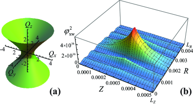
Figure 2: (Color online) (a) – Isofrequency surface for Bragg exciton-polaritons in the linear dissipationless regime at $g\simeq 0$, $\gamma_{0}\simeq 0$. Values of $Q_{X,Y,Z}$ are given in $\sqrt{\eta}$ units. The effective masses of polaritons in the structure are $m_{\|}\approx 3.58\times 10^{-35}\text{kg}$, $m_{\perp}\approx-3.58\times 10^{-36}\text{kg}$. (b) – Normalized probability density $\varphi_{\mathrm{xw}}^{2}$ vs spatial $R$ and $Z$ variables; ${(R-R_{0})^{2}}=(X-X_{0})^{2}+(Y-Y_{0})^{2}$. The parameters are: ${\Delta=6\times 10^{-4}}$, ${Z_{0}=L_{Z}/2}$, ${R_{0}=L_{R}/2=L/\sqrt{2}}$, ${L_{Z}\approx 5.1\times 10^{-4}}$, ${L\approx 3.2\times 10^{-3}}$, ${\eta\approx 2.6\times 10^{7}}$, ${N_{\mathrm{in}}\approx 1.98\times 10^{7}}$. Values of the parameters (except $\Delta$) are taken the same as for Fig. 3 and are discussed below.

We transform Eq. (3) to the standard Schrödinger equation by introducing new variable $\Psi(\mathbf{r},t)=\phi(\mathbf{r},t)e^{-\gamma_{0}t}$ as

$$i\partial_{t}\phi=\left[-\frac{\hbar}{2m_{\|}}\Delta_{\|}+\frac{\hbar}{2m}\partial_{zz}+p(t)^{-1}g|\phi|^{2}\right]\phi,$$ (4)

where we denote $m\equiv|m_{\perp}|$. In (4) we suppose that $e^{-{2\gamma_{0}}t}\approx 1-2\gamma_{0}t\equiv p(t)^{-1}$, cf. PhysLettA37630572012 . This approach is applicable in the limit of weak decay: $\gamma_{0}\ll\Omega_{P}$. We focus on the stationary states of LB polaritons representing the solution of Eq. (4) in the form

$$\varphi(X,Y,Z)=\sqrt{\frac{\kappa^{2}\kappa_{z}}{p(t)^{3}}}\phi(\mathbf{r},t)\\ \times\exp\left[i\frac{\gamma_{0}m_{\|}p(t)}{\hbar}\left(x^{2}+y^{2}-\frac{m}{m_{\|}}z^{2}\right)+iEp(t)t\right],$$ (5)

where $\kappa=\sqrt{\left.\hbar V\right/2m_{\|}g}$, $\kappa_{z}=\sqrt{\left.\hbar V\right/2mg}$ are characteristic macroscopic scales of polaritonic system in the structure, $V=L_{x}L_{y}L_{z}$ is volume of the structure in Fig. 1, $E$ is energy of the system. Substituting (5) for (4) we finally obtain

$$\partial_{ZZ}\varphi-(\partial_{XX}+\partial_{YY})\varphi-\eta\varphi+G\varphi^{3}=0,$$ (6)

where $\eta=\left.EV\right/g$, $G=\left.V\right/\kappa^{2}\kappa_{z}$. Polariton WF $\varphi$ obviously obeys a normalization condition

$$\left.\int_{0}^{L}dX\int_{0}^{L}dY\int_{0}^{L_{Z}}\varphi^{2}dZ\right|_{t=0}\simeq N_{\mathrm{in}},$$ (7)

where $N_{\mathrm{in}}$ is initial (at ${t=0}$) total number of polaritons, the dimensionless variables $X=p(t)x/\kappa$, $Y=p(t)y/\kappa$, $Z=p(t)z/\kappa_{z}$; $\bar{t}=p(t)t$; $L_{X}=L_{Y}=L$ and $L_{Z}$ are characteristic dimensionless lengths of the structure.

Linear regime. The most interesting features of Eq. (6) can be elucidated in the linear regime, i.e. for the ideal gas of non-interacting polaritons occurring at $g\simeq 0$ ($\Omega_{P}/\Omega_{B}\rightarrow 0$) and for the vanishing decay rate $\gamma_{0}\simeq 0$. In this limit, effective dispersion relation is obtained from Eq. (6) substituting plane wave solution $\Psi\propto e^{i\mathbf{QR}}$ : ${\eta=Q_{X}^{2}+Q_{Y}^{2}-Q_{Z}^{2}}$. The corresponding dispersion surface is shown in Fig. 2(a). It is clearly seen that a Bragg mirror allows existence of freely propagating LB polaritons. The specific dispersion of Bragg polaritons leads to the characteristic HMM divergence of the photonic density of states ContemporaryPhysics542732013 . In the same limit, Eq. (6) supports so called X-wave solution defined as PRL901704062003

$$\varphi_{\mathrm{xw}}=\mathbb{C}\text{Re}\left[v^{-1/2}\exp\left[-i\sqrt{v}\right]\right],$$ (8)

where we have redefined $v=\eta[(\Delta-i(Z-Z_{0}))^{2}+(X-X_{0})^{2}+(Y-Y_{0})^{2}]$; $\Delta$ is a real-valued arbitrary coefficient that determines the wave packet localization, $X_{0}$, $Y_{0}$ and $Z_{0}$ define positions of the center of the wave packet, $\mathbb{C}$ is normalization constant which can be estimated using the normalization condition (7). The solution (8) is shown in Fig. 2(b) for the parameters given above. Physically, the polaritonic X-wave represents a nondiffracted localized wave packet analogous to diffractionless beams in optics PRL5814991987 .

Polariton Higgs field. The behavior of our polariton system is essentially modified in the presence of polariton-polariton scattering, i.e. at $g\neq 0$. Equation (6) with the “time” variable $Z$ represents Ginzburg-Landau-Higgs (GLH) equation, that is typically discussed in connection with the Universe properties and bubble evolution PhysRepC3511978 . In order to study Eq. (6) it is conveninent to represent the Higgs field $\varphi$ as a complex scalar field $\varphi=\varphi_{1}+i\varphi_{2}$. The “Mexican hat” Higgs potential $W\equiv W(\varphi_{1},\varphi_{2})$ is shown in Fig. 3(a). The false vacuum state corresponds to $\varphi=0$ while two real vacuum states are located at $\varphi_{\pm}=\pm\sqrt{\left.\eta\right/G}\equiv\pm s$ RubakovClassicalTheoryofGaugeFields2002 . These two states correspond to two minima of Higgs field potential. The state $\varphi=0$ is unstable vs fluctuations, while the states $\varphi_{\pm}$ are stable. The behavior of a polariton system governed by Eq. (6) can be easily understood if we consider small perturbations $\tilde{\varphi}_{1,2}$ defined by $\varphi_{1}=\varphi_{0}+\tilde{\varphi}_{1}$, $\varphi_{2}=\tilde{\varphi}_{2}$ (${\ \tilde{\varphi}_{1,2}\ll\varphi_{0}}$) where $\varphi_{0}$ is the ground state solution of Eq. (6).

Taking into account the global $U(1)$ symmetry properties of the Lagrangian for Eq. (6) it is possible to conclude that the field $\tilde{\varphi}_{1}$ possess a mass whereas the field $\tilde{\varphi}_{2}$ is massless and represents a Nambu-Goldstone boson. Here we focus on $\varphi_{1}$ field properties. In order, Eq. (6) supports a classical (static) kink or black soliton solution

$$\varphi_{0}(X,Y)=\pm s\tanh\left[\Theta\right],$$ (9)

where ${\Theta\equiv\sqrt{\eta}\left.\left(X-X_{0}+Y-Y_{0}\right)\right/2}$. In (9) the parameters $X_{0}$, $Y_{0}$ characterize the position of the envelope minimum. At $X,Y\rightarrow\infty$ the soliton solution in (9) approaches two vacuum states $\varphi_{\pm}$. Combining (7) and (9) we obtain a condition: $N_{\mathrm{in}}\simeq L_{Z}(L^{2}\eta-8\ln[\cosh[\tilde{L}]])/G$, that determines the critical number of particles required for a kink formation. Here we assume that ${X_{0}=Y_{0}=L/2}$ and introduce the dimensionless parameter ${\tilde{L}=L\sqrt{\eta}/2}$.

The parameter $s=\sqrt{\left.\eta\right/G}$ in Eq. (9) plays a crucial role in the field theory, cf. RubakovClassicalTheoryofGaugeFields2002 . In the limit $s\gg 1$, the soliton can be treated as a classical object. We consider the oscillon field as a small perturbation for $\varphi$-function in $Z$ direction. In order to find it, we represent $\varphi$ in the form $\varphi=\varphi_{0}+\mu\delta\varphi$ ($\tilde{\varphi}_{1}\equiv\mu\delta\varphi$), where the oscillon solution $\delta\varphi=\delta\varphi(X,Y)\cos\left(\tilde{\Omega}(Z-Z_{0})\right)$ characterizes lateral excitations; we assume that the condition $|\varphi_{0}|\gg\mu|\delta\varphi|$ is fulfilled. Substituting $\varphi$ and Eq. (9) in Eq. (6) and linearizing it with respect to $\delta\varphi$, we obtain a Schrödinger-like equation $\hat{F}\delta\varphi(X,Y)=\tilde{\Omega}^{2}\delta\varphi(X,Y)$ for eigenstates ($\delta\varphi$) and eigenvalues ($\tilde{\Omega}$) of the operator $\hat{F}=-\nabla_{\|}^{2}+2\eta-3\eta\text{sech}^{2}[\Theta]$. For $\tilde{\Omega}^{2}=3\eta/2$ the first excited state of the system is given by:

$$\delta\varphi(X,Y)=s\tanh[\Theta]\text{sech}[\Theta].$$ (10)

Figure 3: (Color online) (a) – Schematic of Higgs potential $W$ versus $\varphi_{1}$ and $\varphi_{2}$ variables, (b) – perturbed Higgs field (black soliton) $\varphi^{2}$ and (c) – perturbation $\delta\varphi^{2}$ versus dimensionless spatial coordinates $X$ and $Y$. The parameters are: ${X_{0}=Y_{0}=L/2}$, ${Z=Z_{0}=\pi/2\Omega_{2}}$, ${\mu=0.2}$, ${L_{x}=L_{y}=2\mathrm{\mu}\text{m}}$, ${L_{z}=1\mathrm{\mu}\text{m}}$, ${g/V=2.49\text{neV}}$, ${E_{1}=63.8\text{meV}}$. Upper shadow plane ${\ \phi^{2}=\eta/G}$ in (b) indicates vacuum state solution.

The classical kink state $\varphi_{0}$ becomes perturbed due to low amplitude oscillations (fluctuations) of the Higgs field $\varphi$; the state being called “Higgs oscillon”.

In Fig. 3(b) the perturbed kink $\varphi^{2}$ as a function of $X$ and $Y$ at fixed “time” coordinate $Z$ is plotted. At $X\rightarrow\infty$ and $Y\rightarrow\infty$ the black soliton solution approaches two vacuum states $\varphi_{\pm}^{2}$ as the shadow plane in Fig. 3(b) shows. Taking into account a finite size of the lattice in $X$ and $Y$ directions and the periodicity of the system in $Z$ direction (with a period of $2\pi/\tilde{\Omega}$) we consider the oscillon formation in a 3D box $L_{X}\times L_{Y}\times L_{Z}$. We write down the condition $\eta=2\pi^{2}n^{2}/3L_{Z}^{2}$, which is relevant to the normalized energy $\eta\equiv E_{n}V/g$. The square of a quantized Higgs oscillon amplitude $\delta\varphi^{2}$ is plotted in Fig. 3(c) for the ground state $(n=1)$.

Let us note that the energy density $J$ of the polariton Higgs field is $J=\frac{1}{2}[(\partial_{Z}\varphi)^{2}+(\partial_{X}\varphi)^{2}+(\partial_{Y}\varphi)^{2}-\eta\varphi^{2}+\frac{G}{2}\varphi^{4}]$, while the energy density $J_{0}$ of the kink is $J_{0}=\frac{1}{2}\left[(\partial_{X}\varphi_{0})^{2}+(\partial_{Y}\varphi_{0})^{2}-\eta\varphi_{0}^{2}+\frac{G}{2}\varphi_{0}^{4}\right]$. Since ${|\varphi_{0}|\gg\mu|\delta\varphi|}$, $J$ approaches $J_{0}$. Integrating $J_{0}$ over the space coordinates $X$, $Y$ we obtain the energy density in $Z$ direction as

$$E_{0,Z}=\frac{\eta}{3G}\left(2-3\tilde{L}^{2}+8\ln\left[\cosh[\tilde{L}]\right]-2\text{sech}^{2}[\tilde{L}]\right).$$ (11)

The energy density of “vacuum” states $\varphi_{\pm}$ is $J_{\pm}=\frac{1}{2}\left[-\eta\varphi_{\pm}^{2}+\frac{G}{2}\varphi_{\pm}^{4}\right]$. Hence we can write down energy density in $Z$ direction as $E_{\pm,Z}=-\tilde{L}^{2}\eta/G$. Taking into account Eq. (11) we can introduce the so-called “mass” of the kink $M\sim E_{0,Z}-E_{\pm,Z}$. Physically static dark soliton behaves as a relativistic particle with energy $E=Mc^{2}$ at rest, where $c$ is speed of light, cf. PhysRepC3511978 . Note that the “mass” of the soliton $M$ is dependent on the size of the lattice structure.

Topological Schrödinger cat states. Now let us discuss the Higgs field properties beyond the mean field theory. The quantum tunneling between states $\varphi_{\pm}$ representing two minima of the Higgs potential, Fig. 3(a) is responsible for creation of field bubbles in the gauge field theory RubakovClassicalTheoryofGaugeFields2002 . The tunneling leads to formation of the Schrödinger cat states (superposition states):

$$\left|\psi_{\pm}\right\rangle=\frac{1}{\sqrt{2(1+e^{-2s^{2}})}}\left(\left|\phi_{+}\right\rangle\pm\left|\phi_{-}\right\rangle\right),$$ (12)

where $\left|\phi_{+}\right\rangle$ and $\left|\phi_{-}\right\rangle$ are macroscopically distinguishable Glauber’s coherent states associated with fields $\phi_{+}$ and $\phi_{-}$, respectively. The “size of the cat” can be estimated via the overlap integral of the states $|\phi_{\pm}\rangle$ as $\zeta=1/\langle\phi_{+}|\phi_{-}\rangle=e^{2s^{2}}$ PhysRevA5712081998 . The parameter $\zeta$ becomes larger in the limit $s\gg 1$ which is indeed experimentally achievable in realistic structures (9). Notably, the properties of states $\left|\psi_{\pm}\right\rangle$ are highly non-classical, see e.g. PRL57131986 . In particular, due to the interference, a fringe pattern occurs between Gaussian bells representing states $\left|\phi_{\pm}\right\rangle$ in the Wigner function approach. The negativity of this function that is inherent to the states (12) is responsible for that. While the states (12) involve a macroscopically large number of particles they can be used for generation of macroscopic entangled states (cf. PRA4568111992 ) of exciton-polaritons in Bragg-superlattices. The computational qubit states $\left|0\right\rangle$ and $\left|1\right\rangle$ can be associated with mutually orthogonal states (12) as $\left|0\right\rangle=\left|\psi_{+}\right\rangle$ and $\left|1\right\rangle=\left|\psi_{-}\right\rangle$, cf. PRA610423092000 . Alternatively, if the parameter $e^{-2s^{2}}$ in (12) vanishes rapidly, the topological states $\left|\phi_{+}\right\rangle$ and $\left|\phi_{-}\right\rangle$ for the quantum Higgs field itself may be considered as a computational qubit states $\left|0\right\rangle$ and $\left|1\right\rangle$ PRA680423192003 . In this case qubit operations presume implementation of linear circuit networks and conditional photon detection Nature409462001 . Amazingly, such circuits can be designed using well developed semiconductor technologies,  NatCommun417782013 ; PRL1121964032014 .

In conclusion, we propose realisation of quantum HMMs in a periodic planar semiconductor Bragg mirror with embedded QWs. We demonstrate mapping of the polaritonic Gross-Pitaevskii equation onto a nonlinear Ginzburg-Landau-Higgs equation, which exhibits physically non-trivial features. In the liner case, i. e. for non-interacting LB polaritons we obtain a polariton X-wave solution that is reminiscent of a non-diffractive (spatially localized) matter wave packet. We predict formation of kink-shaped states for weakly interacting polaritons. Small amplitude oscillations (oscillons) occur in a perturbed polariton Higgs field due to fluctuations. Going beyond the mean field theory we obtain a Schrödinger cat state as a macroscopic superposition of two vacuum states $\varphi_{\pm}$. Polaritonic nonlinear HMMs have a high potentiality for simulation of fundamental cosmological processes.

- (1) H. Chen, C. Chan, and P. Sheng, Nature Mater. 9, 387 (2010).
- (2) C. Sheng, H. Liu, Y. Wang, S. N. Zhu, and D. A. Genov, Nature Photon. 7, 902 (2013).
- (3) U. Leonhardt, T. Philbin, Progress in Optics 53, 69 (2009).
- (4) M. McCall, Contemporary Physics 54, 273 (2013).
- (5) J. B. Pendry, Phys. Rev. Lett. 85, 3966 (2000).
- (6) J. B. Pendry, A. J. Holden, D. J. Robbins, W. J. Stewart, IEEE Trans. Microwave Theory 47, 2075 (1999).
- (7) A. Poddubny, I. Iorsh, P. A. Belov, Yu. S. Kivshar, Nature Photon. 7, 958 (2013).
- (8) Z. Jacob, J.-Y. Kim, G. V. Naik, A. Boltasseva, E. E. Narimanov, V. M. Shalaev, Appl. Phys. B 100, 215 (2010).
- (9) Z. Liu, H. Lee, Y. Xiong, C. Sun, and Z. Zhang, Science 315, 1686 (2007).
- (10) I. I. Smolyaninov, Phys. Rev. A 88, 033843 (2013).
- (11) V. A. Rubakov, Classical Theory of Gauge Fields (Princeton University Press, Princeton, NJ, 2002).
- (12) E. L. Ivchenko, S. Jorda and A. I. Nesvizhskii, Fiz.Tverd. Tela 36, 2118 (1994) [Phys. Solid State 36, 1156 (1994)].
- (13) A. V. Kavokin and M. A. Kaliteevski, J. Appl. Phys. 79, 595 (1996).
- (14) A. Yu. Sivachenko, M. E. Raikh, and Z. V. Vardeny, Phys. Rev. A 64, 013809 (2001).
- (15) F. Biancalana, L. Mouchliadis, C. Creatore, et al., Phys. Rev. B 80, 121306(R) (2009); C. Creatore, L. Mouchliadis, F. Biancalana, S. Osborne and W. Langbein, J. Phys.: Conf. Ser. 210, 012034 (2010).
- (16) A. Kavokin, J. J. Baumberg, G. Malpuech, and F. P. Laussy, Microcavities (Cambridge University Press, 2007).
- (17) A. Askitopoulos, L. Mouchliadis, I. Iorsh, et al., Phys. Rev. Lett. 106, 076401 (2011).
- (18) M. V. Charukhchyan, E. S. Sedov, S. M. Arakelian, and A. P. Alodjants, Phys. Rev. A. 89, 063624 (2014).
- (19) See supplemental material for the methods used to obtain dependencies in Fig. 1 and Gross-Pitaevskii equation for Bragg exciton-polaritons.
- (20) M. Onorato, D. Proment, Phys. Lett. A 376, 3057 (2012).
- (21) C. Conti, S. Trillo, P. Di Trapani, G. Valiulis, A. Piskarskas, O. Jedrkiewicz, and J. Trull, Phys. Rev. Lett. 90, 170406 (2003); C. Conti, Phys. Rev. E 68, 016606 (2003).
- (22) J. Durnin, J. J. Miceli, and J. H. Eberly, Phys. Rev. Lett. 58, 1499 (1987).
- (23) V. G. Makhankov, Phys. Rep. C 35, 1 (1978).
- (24) J. I. Cirac, M. Lewenstein, K. Molmer, and P. Zoller, Phys. Rev. A 57, 1208 (1998).
- (25) B. Yurke, D. Stoler, Phys. Rev. Lett. 57, 13 (1986).
- (26) B. C. Sanders, Phys. Rev. A 45, 6811 (1992).
- (27) M. C. de Oliveira, W. J. Munro, Phys. Rev. A 61, 042309 (2000).
- (28) T. C. Ralph, A. Gilchrist, and G. J. Milburn, W. J. Munro, S. Glancy, Phys. Rev. A 68, 042319 (2003).
- (29) E. Knill, R. Lafamme, G. J. Milburn, Nature 409, 46 (2001).
- (30) D. Ballarini, M. De Giorgi, E. Cancellieri, R. Houdré, E. Giacobino, R. Cingolani, A. Bramati, G. Gigli, and D. Sanvitto, Nature Commun. 4, 1778 (2013); M. De Giorgi et al., Phys. Rev. Lett. 109, 266407 (2012).
- (31) S. S. Demirchyan, I. Yu. Chestnov, A. P. Alodjants, M. M. Glazov, and A. V. Kavokin, Phys. Rev. Lett. 112, 196403 (2014).