Separatrix splitting at a Hamiltonian $0^{2}i\omega$ bifurcation

Abstract

We discuss the splitting of a separatrix in a generic unfolding of a degenerate equilibrium in a Hamiltonian system with two degrees of freedom. We assume that the unperturbed fixed point has two purely imaginary eigenvalues and a double zero one. It is well known that an one-parametric unfolding of the corresponding Hamiltonian can be described by an integrable normal form. The normal form has a normally elliptic invariant manifold of dimension two. On this manifold, the truncated normal form has a separatrix loop. This loop shrinks to a point when the unfolding parameter vanishes. Unlike the normal form, in the original system the stable and unstable trajectories of the equilibrium do not coincide in general. The splitting of this loop is exponentially small compared to the small parameter. This phenomenon implies non-existence of single-round homoclinic orbits and divergence of series in the normal form theory. We derive an asymptotic expression for the separatrix splitting. We also discuss relations with behaviour of analytic continuation of the system in a complex neighbourhood of the equilibrium.

1 Set up of the problem

Normal form theory provides a powerful tool for studying local dynamics near equilibria. The normal form theory uses coordinate changes in order to represent equations in the simplest possible form. The normal form often possesses additional symmetries which are not present in the original system. For a Hamiltonian system a continuous family of symmetries implies existence of an additional integral of motion due to Noether theorem. In the case of two degrees of freedom, an additional integral of motion makes the dynamics integrable. In this way the normal form theory looses information on non-integrable chaotic dynamics possibly present in the original system.

The accuracy of the normal form theory depends on the smoothness of the original vector field and, in the analytic theory, the error becomes smaller than any order of a small parameter and in some cases an exponentially small upper bound can be established.

In this paper we illustrate this situation considering a classical generic bifurcation of an equilibrium in an one parameter analytic family of Hamiltonian systems with two degrees of freedom (see e.g. [3]). Let us describe our set up in more details. Let $H_{\mu}=H_{\mu}(x_{1},x_{2},y_{1},y_{2})$ be a real-analytic family of Hamiltonian functions defined in a neighbourhood of the origin in $\mathbb{R}^{4}$ endowed with the canonical symplectic form $\Omega=dx_{1}\wedge dy_{1}+dx_{2}\wedge dy_{2}$. The dynamics are defined via the canonical system of Hamiltonian differential equations

$$\dot{x}_{k}=\frac{\partial H_{\mu}}{\partial y_{k}}\quad\mbox{and}\quad\dot{y}_{k}=-\frac{\partial H_{\mu}}{\partial x_{k}}$$

where $k\in\{1,2\}$. The corresponding flow preserves the Hamiltonian $H_{\mu}$ and symplectic form $\Omega$. It is convenient to write down the Hamiltonian equations in the vector form

$$\dot{\bm{x}}=\mathrm{J}H_{\mu}^{\prime}({\bm{x}})$$ (1)

where $\mathrm{J}$ is the standard symplectic matrix and $\bm{x}=(x_{1},x_{2},y_{1},y_{2})$.

We assume that for $\mu=0$ the origin is an equilibrium of the Hamiltonian system with a pair of purely imaginary eigenvalues $\pm i\omega_{0}$ and a double zero one $\lambda_{0}=0$. More precisely, we assume that $H_{0}^{\prime}(0)=0$ and the Hessian matrix $H^{\prime\prime}_{0}(0)$ is already transformed to the diagonal form $H_{0}^{\prime\prime}(0)=\mathrm{diag}(0,1,\omega_{0},\omega_{0})$, which can be achieved by a linear canonical transformation provided ${\mathrm{J}}H_{0}^{\prime\prime}(0)$ is not semi-simple. Then for any integer $n$ there is an analytic canonical change of variables which transforms the Hamiltonian to the following form

$$H_{\mu}=\frac{y_{1}^{2}}{2}+V_{\mu}(x_{1},I)+R_{\mu}(x_{1},y_{1},x_{2},y_{2})$$ (2)

where $I=\frac{x_{2}^{2}+y_{2}^{2}}{2}$, $V_{\mu}(x_{1},I)$ is polynomial in $x_{1},I$ and $\mu$, and the remainder term $R_{\mu}$ has a Taylor expansion which starts with terms of order $n$, i.e., $R_{\mu}=O(\|\bm{x}\|^{n}+\mu^{n})$. In the analytic case, this remainder can be made even exponentially small [18, 17, 15]. Our assumptions imply that

$$\frac{\partial V_{0}}{\partial x_{1}}(0,0)=\frac{\partial^{2}V_{0}}{\partial x_{1}^{2}}(0,0)=0.$$

Then the lower order terms of $V_{\mu}$ have the form

$$V_{\mu}(x_{1},I)=\omega_{0}I-a\mu x_{1}+b\frac{x_{1}^{3}}{3}+cx_{1}I+\dots$$ (3)

where we have explicitly written down all quadratic and some of the cubic terms. In a generic family $a,b,\omega_{0}\neq 0$. Without loosing in generality and for greater convenience we assume $\omega_{0},a,b>0$.

Since the remainder term in (2) is small, it is natural to make a comparison with the dynamics of the normal form described by the truncated Hamiltonian function

$$\hat{H}_{\mu}=\frac{y_{1}^{2}}{2}+V_{\mu}(x_{1},I).$$ (4)

Obviously, the Poisson bracket $\{\hat{H}_{\mu},I\}=0$ and consequently $I$ is an integral of motion for the normal form. For every fixed $I$ equation (4) represents a natural Hamiltonian system in a neighbourhood of the origin on the $(x_{1},y_{1})$-plane. Depending on the values of $\mu$ and $I$, the potential $V_{\mu}$ takes one of three shapes shown on Figure 1.

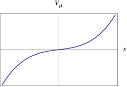
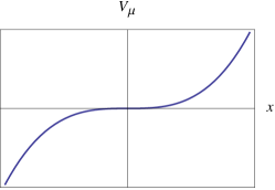
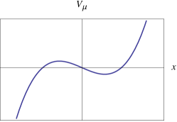
(a)(b)(c)

Figure 1: Potential of the truncated normal form for fixed values of $\mu$ and $I$

Respectively, the equation $\frac{\partial V_{\mu}}{\partial x_{1}}=0$ has either none, one or two solutions located in a small neighbourhood of the origin. These solutions correspond either to a periodic orbit (if $I>0$) or to an equilibrium (if $I=0$) of the normal form. We note that for $I=0$ Figure 1 (a), (b) and (c) correspond respectively to $\mu<0$, $\mu=0$ and $\mu>0$. When the potential has the shape of Figure 1 (c) the corresponding Hamiltonian system has a separatrix loop similar to the one shown on Figure 2.

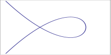
Figure 2: Projection of the separatrix loop on the $(x_{1},y_{1})$-plane

This separatrix loop looks similar to the separatrix of the equation defined by the Hamiltonian

$$\frac{y^{2}}{2}-a\mu x+b\frac{x^{3}}{3}.$$

The situation can be summarised in the following way. The plane $I=0$ is invariant for the normal form Hamiltonian $\hat{H}_{\mu}$. The restriction of the normal form Hamiltonian onto this plane defines a Hamiltonian system with one degree of freedom. As $\mu$ crosses the zero, a pair of equilibria is created on this plane, one saddle point and one elliptic one. The normal form system has a separatrix solution which converges to the saddle equilibrium both at $t\to+\infty$ and $t\to-\infty$. Trajectories located inside this separatrix loop are periodic. All other trajectories escape from a small neighbourhood of the origin and their behaviour cannot be studied using only the local normal form theory presented here.

The remainder term in the Hamiltonian (2) breaks the symmetry of the normal form and it is expected that in general the full equations do not possess neither an additional integral nor an invariant plane [10, 22]. Nevertheless, a part of the normal form dynamics survives. In particular, for $\mu>0$ the Hamiltonian system $H_{\mu}$ has a saddle-centre equilibrium $\bm{p}_{\mu}$ with eigenvalues $\pm\lambda_{\mu}$ and $\pm i\omega_{\mu}$, where $\omega_{\mu}$ is close to $\omega_{0}$ and $\lambda_{\mu}$ is of order of $\mu^{1/4}$. There are 4 solutions (separatrices) of the Hamiltonian system which are asymptotic to this equilibrium. These solutions converge to $\bm{p}_{\mu}$ as $t\to+\infty$ or $t\to-\infty$ and are tangent asymptotically as $t\to\mp\infty$ to eigenvectors of $\mathrm{J}H_{\mu}^{\prime\prime}(\bm{p}_{\mu})$, which correspond to the eigenvalues $\pm\lambda_{\mu}$ respectively.

Two of these separatrices are close to the separatrix loop of the normal form. The main objective of this paper is to study the difference between these separatrices. Our main theorem implies that the unstable solutions returns to a small neighbourhood of $\bm{p}_{\mu}$ but, in general, misses the stable direction by a quantity which is exponentially small compared to $\mu$. Consequently, the system (2) generically does not have a single-round homoclinic orbit for all sufficiently small $\mu>0$. We also point out that our Main theorem implies existence of homoclinic trajectories for Lyapunov periodic orbits located on the central manifold exponentially close to the saddle-centre equilibrium (compare with similar statements for reversible systems in [25] and with the recent preprint [19]).

The dimension arguments [21, 5] show that the existence of a single-round homoclinic orbit to a saddle-centre equilibrium of a vector field in $\mathbb{R}^{4}$ is expected to be a phenomenon of co-dimension between one and three depending on the presence (or absence) of Hamiltonian structure and reversible symmetries. In particular, the codimension one corresponds to a symmetric homoclinic orbit for a symmetric equilibrium in a reversible Hamiltonian system, and the codimension three corresponds to a non-symmetric homoclinic orbit to a symmetric equilibrium in a reversible non-Hamiltonian system. Treating $\lambda$ and $\omega$ as independent parameters, Champneys [5] provided an example of a reversible vector field where lines of homoclinic points bifurcate from $\lambda=0$ on the plane of $(\lambda,\omega)$.

The splitting of the one-round separatrix loop does not prevent existence of “multi-round” homoclinics, i.e., homoclinic orbits which make several rounds close to the separatrix of the normal form before converging to the equilibrium. Generically, if the system is both Hamiltonian and reversible, we expect the existence of reversible multi-round homoclinics for a sequence of values of the parameter $\mu$ which converges to $0$. The study of these phenomena is beyond the goals of this paper.

Since in the limit $\mu\to+0$ the separatrix loop disappears and the ratio $\omega_{\mu}/\lambda_{\mu}\to+\infty$, the problem of the separatrix splitting near the bifurcation can be attributed to the class of singularly perturbed systems characterised by the presence of two different time-scales, similar to the problems considered in [10, 11, 22]. The difficulty of a singularly perturbed problem is related to the exponential smallness of the separatrix splitting in the parameter $\mu$ which requires development of specially adapted perturbation methods (see for example [28, 25, 6] and references in the review [8]).

The difficulties related to the exponential smallness do not appear in problems of the regular perturbation theory. At the same time dynamics of such systems share many qualitative properties with the singularly perturbed case.

If a reversible Hamiltonian system has a symmetric separatrix loop associated with a symmetric saddle-center equilibrium, then its one-parameter reversible Hamiltonian unfolding has multi-round homoclinic orbits for a set of parameter values which accumulate at the critical one [26, 14].

A generic two parameter unfolding of a Hamiltonian system which has a homoclinic orbit to a saddle-centre equilibrium was studies in [20], where countable sets of parameter values for which 2-round (and multi-round) loops are found.

The splitting of the separatrix loop has important consequences for the dynamics. The problem of constructing a complete description of the dynamics in a neighbourhood of a homoclinic loop to a saddle-centre was stated and partially solved in [23]. Later this result was extended and improved in [21, 14, 26].

These papers do not directly cover the situation described in this paper (see [22] for a discussion of relations between these two classes in the Hamiltonian context). The main difference is related to the exponential smallness of the separatrix splitting in the bifurcation problem discussed in the present paper. The presence of exponentially small phenomena hidden beyond all orders of the normal form theory is also observed in other bifurcation problems (see for example [25, 7, 9, 2]).

Finally, we note that the problem of existence of small amplitude single- and multi-round homoclinic orbits arises in various applications. These applications include dynamics of the three-body-problem near $L_{2}$ libration point [24]. Homoclinic solutions also appear in the study of traveling wave or steady-state reductions of partial differential equations on the real line which model various phenomena in mechanics, fluids and optics (for more details see [4, 5]). These solutions are of particular interest as they represent localized modes or solitary waves, these problems are often of the singular perturbed nature [1].

2 Symplectic approach to measuring the separatrix splitting

Let $\bm{p}_{\mu}$ be an equilibrium of the Hamiltonian system with eigenvalues $(\pm\lambda_{\mu},\pm i\omega_{\mu})$. Then for each $\mu\in(0,\mu_{0})$ (where $\mu_{0}$ is a positive constant) there is an analytic change of variables such that the equilibrium is shifted to the origin and the Hamiltonian function is transformed to its Birkhoff normal form which can be presented in the form

$$H_{\mu}=h_{\mu}(E_{h},E_{e})$$ (5)

where $h_{\mu}$ is an analytic function of two variables

$$E_{h}=x_{1}y_{1}\qquad\mbox{and}\qquad E_{e}=\frac{x_{2}^{2}+y_{2}^{2}}{2}.$$ (6)

A statement equivalent to the convergence of the normal form was originally obtained in [27]. Of course, since $\lambda_{\mu}\to 0$ as $\mu\to+0$, the size of domains of convergence shrinks to zero both for the normal form and for the normalising transformation. Nevertheless, it is possible to refine the estimates of [13] in order to establish that the sizes of the domains are sufficiently large to be used in the following arguments.

Obviously $\{E_{h},h_{\mu}\}=\{E_{e},h_{\mu}\}=0$ and, consequently, both $E_{h}$ and $E_{e}$ are constant along trajectories of the Hamiltonian system. Both functions are local integrals only and in general do not have a single-valued extension onto the phase space. The transformation which transforms the original Hamiltonian to the normal form is not unique. Nevertheless the values of $E_{h}$ and $E_{u}$ are unique as they do not depend on this freedom.

As the eigenvalues of the equilibrium are preserved, the Taylor expansion of the transformed Hamiltonian has the form

$$h_{\mu}(E_{h},E_{e})=H_{\mu}(\bm{p}_{\mu})+\lambda_{\mu}E_{h}+\omega_{\mu}E_{e}+O(E_{e}^{2}+E_{h}^{2}).$$ (7)

The structure of the phase space in a neighbourhood of the origin is illustrated by Figure 3 where $H=H_{\mu}-H_{\mu}(\bm{p}_{\mu})$. In particular, in the normal form coordinates points with $x_{1}=y_{1}=0$ correspond to Lyapunoff periodic orbits.

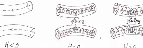
Figure 3: Structure of the phase space in a neighbourhood of a saddle-centre

A trajectory which converges to $\bm{p}_{\mu}$ as $t\to-\infty$ or $t\to\infty$ without leaving the domain of the normal form has $E_{e}=E_{h}=0$. In the normal form coordinates all these trajectories are easy to find explicitly.

Let $\bm{x}_{\mu}^{\pm}(t)$ be separatrix solutions of the Hamiltonian system (2) which converge to the equilibrium

$$\lim_{t\to-\infty}x_{\mu}^{-}(t)=\bm{p}_{\mu}\qquad\mbox{and}\qquad\lim_{t\to+\infty}x_{\mu}^{+}(t)=\bm{p}_{\mu}$$ (8)

being close to the separatrix loop described in the introduction. Since $\bm{x}_{\mu}^{\pm}$ are solutions of an autonomous ODE, these assumptions define the functions $\bm{x}_{\mu}^{\pm}(t)$ up to a translation in time $t$. We will eliminate this freedom later. At the moment it is sufficient to note that $\bm{x}_{\mu}^{\pm}(0)$ will be chosen to be in a small neighbourhood of the intersection of the normal form separatrix with the plane $\Sigma=\{\,y_{1}=0\,\}$. Note that the curve $\bm{x}_{\mu}^{\pm}$ may have more than one intersection with $\Sigma$, in this case we chose a “primary” one.

The unstable separatrix $\bm{x}_{\mu}^{-}(t)$ leaves the domain of the normal form, makes a round trip near the ghost separatrix loop, and at a later moment of time comes back close to the stable direction of the Hamiltonian vector field at $\bm{p}_{\mu}$. Let $E_{e}^{1}$ and $E_{h}^{1}$ be the values of the elliptic and hyperbolic energies obtained after this round-trip. Conservation of the energy implies that $h_{\mu}(E_{h}^{1},E_{e}^{1})=h_{\mu}(0,0)$, so the values of $E_{e}^{1}$ and $E_{h}^{1}$ are not independent. Traditionally the elliptic energy $E_{e}^{1}$ is used to measure the separatrix splitting. In particular, if $E^{1}_{e}=0$, then the trajectory is homoclinic. If $E^{1}_{e}\neq 0$, the trajectory will eventually leave the neighbourhood of $\bm{p}_{\mu}$ for the second time.

Theorem 1 (Main theorem)

There is a sequence of real constants $(a_{k})_{k\geq 0}$ such that

$$E_{e}^{1}\asymp e^{-2\pi\omega_{\mu}/\lambda_{\mu}}\left(a_{0}+\sum_{k\geq 2}a_{k}\lambda_{\mu}^{2k}\right)\,.$$ (9)

The coefficient $a_{0}=|b_{0}|^{2}/2$, where $b_{0}$ is a complex constant defined by the Hamiltonian $H_{0}$ via equation (47) and $a_{n}$ are defined by (51).

We note that $\lambda_{\mu}\sim\mu^{1/4}$ and $\omega_{\mu}=\omega_{0}+O(\mu^{1/2})$. Then the asymptotic expansion (9) implies that $E_{e}^{1}$ is exponentially small compared to $\mu$. Moreover, if $a_{0}\neq 0$ this theorem implies the splitting of the separatrix and, hence, non-existence of a single-loop homoclinic orbit. We do not know an explicit formula to compute $b_{0}$. Nevertheless, numerical methods of [12] can be adapted for evaluating the constants in the asymptotic series with arbitrary precision. The arguments presented in section 9 can be used to prove that $b_{0}$ is generically non-vanishing (as the map $H_{0}\mapsto b_{0}$ is a non-trivial analytic (non-linear) functional). Indeed, if the Hamiltonian $H_{\mu}$ analytically depends on an additional parameter $\nu$, then it can be proved that $b_{0}=b_{0}(\nu)$ is analytic. Then the Melnikov method can be used to show that $b_{0}^{\prime}\neq 0$ for values of $\nu$ which correspond to an integrable Hamiltonian. Finally the analyticity implies that zeroes of $b_{0}(\nu)$ are isolated and, consequently, the coefficient does not vanish for a generic Hamiltonian $H_{0}$.

The proof of the main theorem is based on ideas proposed by V. Lazutkin in 1984 for studying separatrix splitting for the standard map and later used in [6] for studying separatrix splitting of a rapidly forced pendulum. This paper contains a sketch of the proof for the main theorem.

The Melnikov method is often used to study the splitting of separatrices. In general the Melnikov method does not produce a correct estimate for the problem discussed in this paper. Section 9 contains a discussion of the applicability of the Melnikov method.

3 Elliptic energy and the variational equation

As a first step of the proof we provide a description of the elliptic energy $E_{e}^{1}$ in terms of the splitting vector

$$\bm{\delta}_{\mu}(t)=\bm{x}_{\mu}^{+}(t)-\bm{x}_{\mu}^{-}(t),$$ (10)

which describes the difference between the stable and unstable separatrix solution, and a solution of a variational equation around $\bm{x}_{\mu}^{+}(t)$. This description allows us to compute $E^{1}_{e}$ without explicit usage of a transformation to the normal form in a neighbourhood of the saddle-centre equilibrium.

In the normal form coordinates the Hamiltonian is described by equation (5), thus the corresponding equations of motion take the form

$$\dot{x}_{1}=\tilde{\lambda}x_{1},\quad\dot{y}_{1}=-\tilde{\lambda}y_{1},\quad\dot{x}_{2}=\tilde{\omega}x_{2},\quad\dot{y}_{2}=-\tilde{\omega}y_{2},$$ (11)

where $\tilde{\lambda}=\partial_{1}h_{\mu}(E_{h},E_{e})$ and $\tilde{\omega}=\partial_{2}h_{\mu}(E_{h},E_{e})$. Since on the local stable trajectory $E_{h}=E_{u}=0$, equation (7) implies that $\tilde{\lambda}(0,0)=\lambda_{\mu}$, and we can find this trajectory explicitly:

$$\bm{x}_{\mu}^{+}(t)=(0,c_{\mu}e^{-\lambda_{\mu}t},0,0)$$ (12)

where $c_{\mu}$ is a constant. Then the variational equation around this solution takes the form

$$\dot{\xi}_{1}=\lambda_{\mu}\xi_{1}\quad\dot{\eta}_{1}=-\lambda_{\mu}\eta_{1}-\kappa_{\mu}y_{1}^{2}(t)\xi_{1},\qquad\dot{\xi}_{2}=\omega_{\mu}\eta_{2},\qquad\dot{\eta}_{2}=-\omega_{\mu}\xi_{2}$$

where $y_{1}(t)=c_{\mu}e^{-\lambda_{\mu}t}$ and $\kappa_{\mu}=\partial^{2}_{1,1}h_{\mu}(0,0)$. A fundamental system of solutions for the variational equation is found explicitly:

$$\begin{array}[]{ll}\bm{\xi}_{1}(t)=e^{-i\omega_{\mu}t}(0,0,1,-i),&\bm{\xi}_{2}(t)=e^{i\omega_{\mu}t}(0,0,1,i),\\[8.0pt] \bm{\xi}_{3}(t)=\lambda_{\mu}c_{\mu}e^{-\lambda_{\mu}t}(0,1,0,0),&\bm{\xi}_{4}(t)=-\lambda_{\mu}^{-1}c_{\mu}^{-1}(e^{\lambda_{\mu}t},c_{\mu}^{2}\kappa_{\mu}te^{-\lambda_{\mu}t},0,0).\end{array}$$ (13)

Note that we have chosen $\bm{\xi}_{3}(t)=\dot{\bm{x}}_{\mu}^{+}(t)$. The first two solutions are mutually complex conjugate, so real-analytic solutions can be easily constructed when needed. A direct computation shows that $\Omega({\bm{\xi}}_{1},{\bm{\xi}}_{2})=2i$ and $\Omega(\bm{\xi}_{3},\bm{\xi}_{4})=1$. For all other pairs $(j,k)$ the symplectic form $\Omega(\bm{\xi}_{j},\bm{\xi}_{k})$ vanishes. Later we will study those solutions for non-real values of $t$. So it is interesting to note that the function $\bm{\xi}_{1}(t)$ exponentially grows in the complex upper half-plane $\Im t>0$, while $\bm{\xi}_{2}(t)$ exponentially decays there.

For each fixed value of $t$ we can consider the collection of vectors $\bm{\xi}_{k}(t)$, $k=1,\dots,4$, as a basis in $\mathbb{C}^{4}$. Then the function

$$\tilde{\theta}_{1}(t):=\frac{1}{2i}\Omega(\bm{\delta}_{\mu}(t),\bm{\xi}_{2}(t))$$ (14)

provides the $\bm{\xi}_{1}$-component of the splitting vector $\bm{\delta}_{\mu}(t)$. Equations (13) and (12) imply that

$$\tilde{\theta}_{1}(t)=\frac{1}{2i}e^{i\omega_{\mu}t}(ix^{-}_{2}(t)-y^{-}_{2}(t))\,,$$

where $x_{2}^{-}$ and $y_{2}^{-}$ are components of $\bm{x}^{-}_{\mu}$ in the normal form coordinates (for the values of $t$ corresponding to the first return of the unstable trajectory to the small neighbourhood of the saddle-centre $\bm{p}_{\mu}$). Taking into account that $\bm{x}^{-}_{\mu}$ is real-analytic and using the definition of $E_{e}^{1}$ of (6), we obtain that the equality

$$|\tilde{\theta}_{1}(t)|^{2}=\frac{(x_{2}^{-}(t))^{2}+(y_{2}^{-}(t))^{2}}{4}=\frac{E_{e}^{1}}{2}.$$ (15)

holds for real values of $t$. Since $E_{e}^{1}$ is a local integral, $|\tilde{\theta}_{1}(t)|$ also stays constant for real $t$ while the unstable solution remains inside the domain of the normal form.

The equation (15) provides a relation between $E_{e}^{1}$ and $\tilde{\theta}_{1}$. While $E_{e}^{1}$ is defined using the normal form coordinates, the function $\tilde{\theta}_{1}$ is defined by (14) and can be evaluated in other canonical systems of coordinates. This computation relies on accurate analysis of the way the splitting vector $\bm{\delta}_{\mu}$ and the solutions of the variational equation $\bm{\xi}_{k}$ are transformed under coordinate changes. It is important to note that although canonical coordinate changes do preserve the symplectic form, $\Omega(\bm{\delta}_{\mu}(t),\bm{\xi}_{2}(t))$ does not take the same value when evaluated in a different coordinate system but can differ by a value of the order of $\|\bm{\delta}_{\mu}(t)\|^{2}$.

Slightly overloading the notation, let $\bm{\delta}_{\mu}$ and $\bm{\xi}_{k}$ be respectively the splitting vector and the solutions of the variational equation written in the original coordinates. The splitting vector is defined by equation (10). The solutions $\bm{\xi}_{k}$ can be fixed by asymptotic conditions described in the next section to ensure that they represent the same solutions of the variational equation as in (14) but expressed in the other coordinates. Then we define a function in a way similar to (14)

$$\theta_{1}(t)=\frac{1}{2i}\Omega(\bm{\delta}_{\mu}(t),\bm{\xi}_{2}(t)).$$ (16)

It is easy to check that $\tilde{\theta}_{1}(t)=\theta_{1}(t)+O(C_{\mu}\|\delta_{\mu}(t)\|^{2})$, where the constant $C_{\mu}$ bounds the $C^{2}$-norm of the transformation between the systems of coordinates. For the real $t$, the function $\bm{\xi}_{2}(t)$ is uniformly bounded and we conclude that $|\theta_{1}(t)|=O(\|\delta_{\mu}(t)\|)$. We conclude that $|\tilde{\theta}_{1}(t)|^{2}=|\theta_{1}(t)|^{2}+O(C_{\mu}\|\delta_{\mu}(t)\|^{3})$. Then equation (15) implies that

$$E_{e}^{1}=2|\theta_{1}(t)|^{2}+O(C_{\mu}\|\delta_{\mu}(t)\|^{3})\,.$$ (17)

A refinement of the arguments from [13] implies that $C_{\mu}=O(\mu^{-2})$. This factor does not break the approximation as $\theta_{1}$ is of the same order as $\delta_{\mu}$ and $\delta_{\mu}$ is exponentially small compared to $\mu$. We will use the equation (17) to obtain an estimate for $E_{e}^{1}$.

4 Variational equation

On the next step of the proof we study solutions of the variational equation near the unstable separatrix solution $\bm{x}_{\mu}^{-}$:

$$\dot{\bm{\xi}}=\left.\mathrm{J}H_{\mu}^{\prime\prime}\right|_{\bm{x}_{\mu}^{-}(t)}\bm{\xi}\,.$$ (18)

This is a linear homogeneous non-autonomous equation. Since the variational equation comes from a Hamiltonian system, it is easy to check that for any two solutions $\bm{\xi}$ and $\tilde{\bm{\xi}}$ of equation (18) the value of the symplectic form $\Omega(\bm{\xi}(t),\tilde{\bm{\xi}}(t))$ is independent of $t$. This property together with asymptotic behaviour of solutions at $t\to-\infty$ are used to select a fundamental system of solutions.

Let $\bm{v}_{\mu}\in\mathbb{C}^{4}$ be an eigenvector of the linearised Hamiltonian vector field at $\bm{p}_{\mu}$,

$$\left.\mathrm{J}H_{\mu}^{\prime\prime}\right|_{\bm{p}_{\mu}}\bm{v}_{\mu}=i\omega_{\mu}\bm{v}_{\mu},$$

such that $\Omega(\bm{v}_{\mu},\bar{\bm{v}}_{\mu})=-2i$. Note that the complex conjugate vector $\bar{\bm{v}}_{\mu}$ is also an eigenvector, but it corresponds to the complex conjugate eigenvalue $-i\omega_{\mu}$. Let $\bm{v}_{\mu}=\bm{v}_{\mu}^{\prime}+i\bm{v}_{\mu}^{\prime\prime}$ with $\bm{v}_{\mu}^{\prime},\bm{v}_{\mu}^{\prime\prime}$ being vectors with real components. Then our normalisation condition is equivalent to $\Omega(\bm{v}_{\mu}^{\prime},\bm{v}_{\mu}^{\prime\prime})=1$. The vector $\bm{v}_{\mu}$ is defined uniquely up to multiplication by a complex constant of unit absolute value, in other words, for any real $c$ the vector $e^{ic}\bm{v}_{\mu}$ also satisfies our normalisation assumption. We assume that this freedom is eliminated in the same way as in the linear part of the normal form theory near the saddle-centre. In particular, $v_{\mu}$ is a smooth function of $\mu^{1/2}$ (including the limit $\mu\to+0$).

Now we are ready to define fundamental solutions of the variational equation. One solution is selected by the assumption

$$\bm{\xi}_{2}(t)=e^{i\omega_{\mu}t}\bm{v}_{\mu}+O(e^{\lambda_{\mu}t})$$

for $t\to-\infty$. The other one is defined using the real symmetry:

$$\bm{\xi}_{1}(t)=\overline{{\bm{\xi}}_{2}(\bar{t})}\,.$$

These two solutions are not real on the real axis and $\Omega(\bm{\xi}_{1},\bm{\xi}_{2})=2i$. Sometimes it is useful to consider their linear combinations

$$\tilde{\bm{\xi}}_{1}(t)=\frac{\bm{\xi}_{1}(t)+\bm{\xi}_{2}(t)}{2}\qquad\mbox{and}\qquad\tilde{\bm{\xi}}_{2}(t)=\frac{\bm{\xi}_{1}(t)-\bm{\xi}_{2}(t)}{2i}$$

which are real-analytic.

The third solution is given by

$$\bm{\xi}_{3}(t)=\dot{\bm{x}}^{-}_{\mu}(t)\,.$$

The last solution is chosen to satisfy the following normalisation conditions:

$$\Omega(\bm{\xi}_{1},\bm{\xi}_{4})=\Omega(\bm{\xi}_{2},\bm{\xi}_{4})=0,\qquad\Omega(\bm{\xi}_{3},\bm{\xi}_{4})=1.$$

We note that since the original system is Hamiltonian, for any two functions $\bm{\xi}$ and $\tilde{\bm{\xi}}$ which satisfy the variational equation, $\Omega(\bm{\xi}(t),\tilde{\bm{\xi}}(t))$ is independent of $t$. Consequently the vectors $\tilde{\bm{\xi}}_{1}(t)$, $\tilde{\bm{\xi}}_{2}(t)$, $\bm{\xi}_{3}(t)$, $\bm{\xi}_{4}(t)$ form a standard symplectic basis for every $t$:

$$\Omega(\tilde{\bm{\xi}}_{1},\tilde{\bm{\xi}}_{2})=\Omega(\bm{\xi}_{3},\bm{\xi}_{4})=1,\qquad\Omega(\bm{\xi}_{1},\bm{\xi}_{3})=\Omega(\bm{\xi}_{2},\bm{\xi}_{3})=\Omega(\bm{\xi}_{1},\bm{\xi}_{4})=\Omega(\bm{\xi}_{2},\bm{\xi}_{4})=0.$$ (19)

Then we can write the splitting vector in this basis:

$$\bm{\delta}_{\mu}(t)=\tilde{\theta}_{1}(t)\tilde{\bm{\xi}}_{1}(t)+\tilde{\theta}_{2}(t)\tilde{\bm{\xi}}_{2}(t)+\theta_{3}(t)\bm{\xi}_{3}(t)+\theta_{4}(t)\bm{\xi}_{4}(t).$$

The normalisation condition (19) implies that

$$\tilde{\theta}_{1}=\Omega(\bm{\delta}_{\mu},\tilde{\bm{\xi}}_{2}),\quad\tilde{\theta}_{2}=-\Omega(\bm{\delta}_{\mu},\tilde{\bm{\xi}}_{1}),\quad\theta_{3}=\Omega(\bm{\delta}_{\mu},\bm{\xi}_{4}),\quad\theta_{4}=-\Omega(\bm{\delta}_{\mu},\bm{\xi}_{3}).$$

For the future use we also define

$$\theta_{1}=\Omega(\bm{\delta}_{\mu},\bm{\xi}_{2}),\quad\theta_{2}=\Omega(\bm{\delta}_{\mu},\bm{\xi}_{1}),$$

which involve the non-real solutions of the variational equation. The real symmetry implies that $\theta_{2}(t)=\overline{\theta_{1}(\overline{t})}$.

We note that in general the coefficients $\theta_{k}$ depend on time. Indeed, the equation (1) implies that

$$\dot{\bm{\delta}}_{\mu}=\mathrm{J}(H^{\prime}(\bm{x}^{-}_{\mu}+\bm{\delta}_{\mu})-H^{\prime}(\bm{x}^{-}_{\mu}))=\left.\mathrm{J}H^{\prime\prime}\right|_{\bm{x}^{-}_{\mu}}\bm{\delta}_{\mu}+{\bm{F}}_{2}(\bm{x}^{-}_{\mu},\bm{\delta}_{\mu})$$

where $\bm{F}_{2}(\bm{x}^{-}_{\mu},\bm{\delta}_{\mu})=O(\|\bm{\delta}_{\mu}\|^{2})$ is a remainder of a Taylor series. Then differentiating the definition of $\theta_{k}$ with respect to $t$ and taking into account that $\left.\mathrm{J}H^{\prime\prime}\right|_{\bm{x}^{-}_{\mu}}$ is a symplectic matrix we get

$$\dot{\theta}_{k}=\pm\Omega(\bm{F}_{2},\bm{\xi}_{k^{\prime}(k)})=O(\|\bm{\delta}_{\mu}\|^{2})\,,$$

where $k^{\prime}(k)$ is the index of the canonically conjugate variable (e.g. $k^{\prime}(1)=2$ and $k^{\prime}(2)=1$). So $\theta_{k}$ are $\|\bm{\delta}_{\mu}\|^{2}$-close to being constant. Moreover, $\theta_{3},\theta_{4}$ are much smaller than $\theta_{1}$ and $\theta_{2}$. Indeed, taking into account the definition of $\bm{\xi}_{3}$ we get

$$\theta_{4}=-\Omega(\bm{\delta}_{\mu},\bm{\xi}_{3})=-\Omega(\bm{\delta}_{\mu},\dot{\bm{x}}^{-}_{\mu})=d_{\bm{x}^{-}_{\mu}}H_{\mu}(\bm{\delta}_{\mu}),$$

where $d_{\bm{x}^{-}_{\mu}}H_{\mu}$ is the differential of $H_{\mu}$ at the point ${\bm{x}^{-}_{\mu}}$. Since $H(\bm{x}^{-}_{\mu}+\bm{\delta})=H(\bm{x}^{+}_{\mu})=H(\bm{x}^{-}_{\mu})$, we conclude that $\theta_{4}=O(\|\bm{\delta}_{\mu}\|^{2})$.

Initial condition for $\bm{x}_{\mu}^{\pm}(0)$ can be chosen in such a way that $\Omega(\bm{\delta}_{\mu}(0),\bm{\xi}_{3}(0))=0$ (by translating time in the stable solution in order to achieve the zero projection of $\bm{\delta}_{\mu}(0)$ on the direction of the Hamiltonian vector field at $\bm{x}^{-}(0)$ represented by $\bm{\xi}_{3}(0)$). Thus $\theta_{3}=O(\|\bm{\delta}\|^{2})$.

Taking into account the real symmetry we see that the problem of the separatrix splitting is reduced to the study of a single complex constant $\theta_{1}(0)$ (via the equation (17)).

5 Formal expansions

The proof of the main theorem requires construction of accurate approximations for the stable and unstable separatrix solutions of the Hamiltonian system (1) as well as the fundamental solutions of the variational equation (18). Taking into account that the Hamiltonian (2) can be formally transformed to the integrable normal form (4), we construct an approximation by finding a formal solution to the systems defined by the normal form Hamiltonian. Of course, the series of the normal form theory diverge in general, but they can be shown to provide asymptotic expansions for the true solutions restricted to properly chosen domains on the complex plane of the time variable $t$.

5.1 Formal separatrix

In this section we find a formal separatrix for the normal form Hamiltonian

$$\hat{H}_{\mu}=\frac{y_{1}^{2}}{2}+\hat{V}_{\mu}(x_{1},I)$$ (20)

where $\hat{V}_{\mu}$ is a formal series in three variables $x_{1},I$ and $\mu$ with the lower order terms given by (3). The corresponding Hamiltonian system has the form

$$\begin{array}[]{ll}\dot{x}_{1}=y_{1},&\dot{x}_{2}=\partial_{2}\hat{V}_{\mu}(x_{1},I)y_{2},\\[8.0pt] \dot{y}_{1}=-\partial_{1}\hat{V}_{\mu}(x_{1},I),&\dot{y}_{2}=-\partial_{2}\hat{V}_{\mu}(x_{1},I)x_{2}.\end{array}$$ (21)

Obviously, the plane $x_{2}=y_{2}=0$ is invariant and we construct a formal separatrix located on this plane. Formal expansions can be substantially simplified with the help of an auxiliary small parameter $\varepsilon$. So instead of performing expansion directly in powers of $\mu$, we look for a solution of the system (21) considering $x_{1},$ $y_{1}$ and $\mu$ as formal power series in $\varepsilon$. The coefficients of the series for $x_{1}$ and $y_{1}$ are assumed to be functions of the slow time $s=\varepsilon t$. The following lemma establishes existence and uniqueness of a formal solution in a specially designed class of formal series.

It is important to note that the leading terms in the series $\hat{x}_{1}$ and $\hat{y}_{1}$ are of the form $\varepsilon^{2}p_{1}(s)$ and $\varepsilon^{3}q_{1}(s)$ respectively. This choice makes the expansions of Lemma 2 compatible with approximations for the separatrix obtained using the standard scaling, a traditional tool used in the bifurcation theory.

Lemma 2

There are unique real coefficients $p_{k,l}$, $q_{k,l}$ and $\mu_{k}$ such that the formal series

$$\hat{x}_{1}=\sum_{k\geq 1}\varepsilon^{2k}p_{k}(\varepsilon t),\qquad\hat{y}_{1}=\sum_{k\geq 1}\varepsilon^{2k+1}q_{k}(\varepsilon t),\qquad\mu=\sum_{k\geq 2}\mu_{k}\varepsilon^{2k},$$ (22)

where $p_{1}(s)$ is not constant and the coefficients $p_{k}$, $q_{k}$ with $k\geq 1$ have the form

$$p_{k}(s)=\sum_{l=0}^{k}\frac{p_{k,l}}{\cosh^{2l}\tfrac{s}{2}},\qquad q_{k}(s)=\sum_{l=1}^{k}\frac{q_{k,l}\sinh\tfrac{s}{2}}{\cosh^{2l+1}\tfrac{s}{2}},$$ (23)

together with $x_{2}=y_{2}=0$ satisfy the Hamiltonian equations (21). Moreover, if $\hat{H}_{\mu}$ is a formal normal form for the analytic family $H_{\mu}$ defined by (2), then the series for $\mu$ are convergent and $\varepsilon=\lambda_{\mu}$.

Proof. The restriction of the system (21) onto the invariant plane $x_{2}=y_{2}=0$ is equivalent to a single equation of the second order

$$\varepsilon^{2}x^{\prime\prime}+\partial_{x}\hat{V}_{\mu}(x)=0,$$

where ^′ denotes differentiation with respect to the variable $s=\varepsilon t$ and $\hat{V}_{\mu}(x)$ is used to denote the formal series $\hat{V}_{\mu}(x,0)$. Our assumptions on the lower order terms of the Hamiltonian $\hat{H}_{\mu}$ imply that

$$\hat{V}_{\mu}(x)=\sum_{k,l\geq 0}v_{kl}\mu^{k}x^{l}$$

with $v_{00}=v_{01}=v_{02}=0$ and $v_{03}v_{11}\neq 0$. Multiplying the differential equation by $x^{\prime}$ and integrating once we get

$$\varepsilon^{2}(x^{\prime})^{2}+2\hat{V}_{\mu}(x)+C_{\varepsilon}=0$$

where $C_{\varepsilon}$ is a formal series in $\varepsilon^{2}$ (the first two terms in the sum are power series in $\varepsilon^{2}$ by the assumptions of the lemma, so $C_{\varepsilon}$ must be in the same class). This equation has a unique formal solution of the form

$$x=\sum_{n\geq 1}\varepsilon^{2n}p_{n}(z),\qquad\mu=\sum_{n\geq 2}\mu_{n}\varepsilon^{2n},\qquad C_{\varepsilon}=\sum_{n\geq 6}C_{n}\varepsilon^{2n},$$

where $p_{n}$ is polynomial of order $n$ in $z=\frac{1}{\cosh^{2}\frac{s}{2}}$. Indeed, differentiating $x$ with respect to $s$ we get

$$x^{\prime}=\sum_{n\geq 1}\varepsilon^{2n}p_{n}^{\prime}z^{\prime}$$

and taking the square

$$(x^{\prime})^{2}=\sum_{n_{1},n_{2}\geq 1}\varepsilon^{2n_{1}+2n_{2}}p^{\prime}_{n_{1}}p^{\prime}_{n_{2}}z^{2}(1-z)$$

where we used the identity $(z^{\prime})^{2}=z^{2}-z^{3}$. Substituting the formal series $x$ and $\mu$ we get

$$\hat{V}_{\mu}(x)=\sum_{k,l\geq 0}v_{kl}\sum_{\begin{subarray}{c}\bm{j}\geq 2,\,\bm{i}\geq 1\end{subarray}}\varepsilon^{2(j_{1}+\dots j_{k}+i_{1}+\dots+i_{l})}\mu_{j_{1}}\dots\mu_{j_{k}}p_{i_{1}}\dots p_{i_{l}}\,.$$

After substituting these expressions into the equation we get

$$\sum_{n_{1},n_{2}\geq 1}\varepsilon^{2n_{1}+2n_{2}+2}p^{\prime}_{n_{1}}p^{\prime}_{n_{2}}(z^{2}-z^{3})+2\sum_{k,l\geq 0}v_{kl}\sum_{\bm{j}\geq 2,\,\bm{i}\geq 1}\varepsilon^{2(j_{1}+\dots j_{k}+i_{1}+\dots+i_{l})}\mu_{j_{1}}\dots\mu_{j_{k}}p_{i_{1}}\dots p_{i_{l}}+\sum_{k\geq 3}\varepsilon^{2k}C_{k}=0.$$

This equality is treated in the class of formal series in powers of $\varepsilon^{2}$. The leading order is of order of $\varepsilon^{6}$. Collecting all terms of this order we get

$$(p^{\prime}_{1})^{2}(z^{2}-z^{3})+2v_{03}p_{1}^{3}+2v_{11}\mu_{2}p_{1}+C_{3}=0\,.$$

Looking for $p_{1}$ in the form $p_{1}=p_{10}+p_{11}z$ we get

$$p_{11}^{2}(z^{2}-z^{3})+2v_{03}(p_{10}^{3}+3p_{10}^{2}p_{11}z+3p_{10}p_{11}^{2}z^{2}+p_{11}^{3}z^{3})+2v_{11}\mu_{2}(p_{10}+p_{11}z)+C_{3}=0.$$

This equation is equivalent to the following system for the coefficients:

$$-p_{11}^{2}+2v_{03}p_{11}^{3}=0,\qquad p_{11}^{2}+6v_{03}p_{10}p_{11}^{2}=0,\qquad v_{03}3p_{10}^{2}p_{11}+2v_{11}\mu_{2}p_{11}=0,\qquad 2v_{03}p_{10}^{3}+C_{3}=0.$$

This system has a unique solution with $p_{11}\neq 0$, which leads to a non-constant $p_{1}$:

$$p_{11}=(2v_{03})^{-1},\quad p_{10}=-(6v_{03})^{-1},\quad\mu_{2}=(24v_{03}v_{11})^{-1},\quad C_{3}=-2v_{03}p_{10}^{3}.$$

Then we continue by induction. Suppose that for some $n\geq 2$ all coefficients are defined uniquely up to $p_{n-1}$, $\mu_{n}$ and $C_{n+1}$. Then collect the terms of order $\varepsilon^{2n+4}$ to obtain an equation of the form

$$2p_{11}p_{n}^{\prime}(z^{2}-z^{3})=3v_{03}p_{1}^{2}p_{n}+v_{11}\mu_{2}p_{n}+v_{11}\mu_{n+1}p_{1}+C_{n+2}+pol_{n+2},$$

where $pol_{n+2}$ is a polynomial of order $n+2$ in $z$ with coefficients depending on already known ones. We can find the coefficients of $p_{n}$ starting from the largest power of $z$. We find $\mu_{n+1}$ from the linear term in $z$ and $C_{n+2}$ from the constant term. In the essence we solve a linear algebraic system with a triangle matrix with non-vanishing elements on the diagonal. So the coefficients are unique.

If $H_{\mu}$ is an analytic family defined by (2) then there is an analytic coordinate change which moves the remainder term $R_{\mu}$ beyond any fixed order $n$. Neglecting this remainder we obtain a polynomial Hamiltonian of the form (4) and it is not too difficult to verify that for this Hamiltonian $\varepsilon=\tilde{\lambda}_{\mu}$ where $\tilde{\lambda}_{\mu}$ is an exponent of the saddle-centre equilibrium of the truncated normal form. Since $\lambda_{\mu}$ is not changed by smooth coordinate changes, the Taylor expansions of $\tilde{\lambda}_{\mu}$ and $\lambda_{\mu}$ in powers of $\mu^{1/4}$ coincide in the first $n$ terms (indeed, our formal computations show that the first $n$-terms of this series are uniquely determined by the first $n$ orders of the Hamiltonian, these terms are the same as the remainder affects terms of higher order only).   

5.2 Formal variational equation

In addition to the formal separatrix solution we will need to study formal solutions for the corresponding variational equation. These formal solutions will be used to approximate analytic solutions of the variational equation with an error being of a sufficiently high order in $\varepsilon$.

The variational equation near the formal solution provided by Lemma 2 has the form

$$\begin{array}[]{ll}\dot{x}_{1}=y_{1},&\dot{x}_{2}=\partial_{2}\hat{V}_{\mu}(\hat{x}_{1},0)y_{2},\\[8.0pt] \dot{y}_{1}=-\partial_{1}\hat{V}_{\mu}(\hat{x}_{1},0)x_{1},&\dot{y}_{2}=-\partial_{2}\hat{V}_{\mu}(\hat{x}_{1},0)x_{2}.\end{array}$$ (24)

This system is split into two independent pairs of linear equations. This property allows us to solve this system explicitly. Indeed, a direct substitution shows that the function

$$\hat{\bm{\xi}}=(0,0,1,i)\exp\left(i\int_{0}^{t}\partial_{2}\hat{V}_{\mu}(\hat{x}_{1},0)\right)$$

satisfies the system (24). In order to give precise meaning to this expression in the class of formal series we define the first formal solution of the formal variational equation by

$$\hat{\bm{\xi}}_{2}=(0,0,1,i)\exp i\hat{u}_{\mu}$$ (25)

where the formal series $\hat{u}_{\mu}$ is defined by termwise integration

$$\hat{u}_{\mu}:=\int_{0}^{t}\partial_{2}\hat{V}_{\mu}(\hat{x}_{1},0)=\omega_{\mu}t+\sum_{k\geq 0}\varepsilon^{2k+1}u_{k}(\varepsilon t)$$ (26)

where

$$u_{k}(s)=\sum_{l=0}^{k}u_{k,l}\frac{\sinh\tfrac{s}{2}}{\cosh^{2l+1}\tfrac{s}{2}},\qquad\omega_{\mu}=\sum_{k\geq 0}\omega_{k}\varepsilon^{2k}\,,$$ (27)

and $u_{k,l}$, $\omega_{k}$ are real coefficients. These coefficients can be computed by substituting the formal series $\hat{x}_{1}$ into $\partial_{1}\hat{V}_{\mu}(x_{1},0)$ and integrating the result termwise.

The other solution $\hat{\bm{\xi}}_{1}$ is defined using the real symmetry: $\hat{\bm{\xi}}_{1}(t)=\overline{\hat{\bm{\xi}}_{2}(\overline{t})}$.

The third solution is obtained by differentiating the formal separatrix with respect to $t$:

$$\hat{\bm{\xi}}_{3}=(\dot{\hat{x}}_{1},\dot{\hat{y}}_{1},0,0)\,.$$

Finally, the fourth solution is found from the normalisation assumptions

$$\Omega(\hat{\bm{\xi}}_{1},\hat{\bm{\xi}}_{4})=\Omega(\hat{\bm{\xi}}_{2},\hat{\bm{\xi}}_{4})=0,\quad\Omega(\hat{\bm{\xi}}_{3},\hat{\bm{\xi}}_{4})=1.$$

We sketch the derivation for its form. A solution to the equation

$$\left|\begin{array}[]{ll}\hat{x}_{1}^{\prime}&\hat{v}\\ \hat{x}_{1}^{\prime\prime}&\hat{v}^{\prime}\end{array}\right|=1$$

also satisfies the same variational equation as $\hat{x}_{1}^{\prime}$. Looking for a formal solution of the form

$$\hat{v}=\sum_{k\geq 0}\varepsilon^{2k}v_{k}$$

with

$$v_{0}=c_{0}sz^{\prime}+z^{-1}d_{2}(z)\qquad\mbox{and}\qquad v_{k}=c_{k}(z)sz^{\prime}+z^{-1}d_{k+2}(z)$$ (28)

where $d_{k}$, $c_{k}$ are polynomial in $z=\frac{1}{\cosh^{2}\frac{s}{2}}$ (of the order indicated by the subscript). Substituting the series into the equation and collecting the leading terms in $\varepsilon$, we get

$$z^{\prime}v_{0}^{\prime}-z^{\prime\prime}v_{0}=p_{11}^{-1}.$$

This equation can be solved explicitly:

$$v_{0}=\left(-1/2z^{-1}+15/8(sz^{\prime}+2z-2/3)\right)p^{-1}_{11}\,.$$

The solution of the equation is defined up to adding a multiple of $z^{\prime}$, which satisfies the corresponding homogeneous equation, but only one of those solutions has the desired form (28). Thus our expression for $v_{0}$ provides the unique solution in our class.

Acting in a similar way and collecting terms of order $\varepsilon^{2n}$ we get an equation for $v_{n}$ with $n\geq 1$:

$$\sum_{0\leq k\leq n}\bigl{(}p_{n-k}^{\prime}v_{k}^{\prime}-p_{n-k}^{\prime\prime}v_{k}\bigr{)}=0\,,$$

where $p_{k}(s)$ are defined by equation (23). An induction in $n$ can be used to prove that this equation uniquely determines a function $v_{n}$ of the form (28) provided $v_{k}$ with $k<n$ already have that form. The induction step is rather straightforward: we plug (28) into the equation and take into account that $p_{k}$ is a polynomial in $z$ of order $k$, then $c_{n}^{\prime}$ is determined by the terms proportional to $s$. The constant term of $c_{n}$ is used to satisfy a compatibility condition in a system for coefficients of $d_{n+2}$. The identities $(z^{\prime})^{2}=z^{2}-z^{3}$, $z^{\prime\prime}=z-\frac{3}{2}z^{2}$ are used to simplify equations.

5.3 Re-expansion near the singularity at $s=i\pi$.

It is easy to see that all coefficients of the series (22) converge to a constant both for $t\to+\infty$ and for $t\to-\infty$. So any partial sum of the series represents a closed loop on the plane $(x_{1},y_{1})$. We say that the series represent a formal (or ghost) separatrix as the series are expected to diverge generically. It can be shown that the same series provide an asymptotic expansions both for the stable and unstable solution of the original system (after reversing the transformation which brings the original Hamiltonian to the formal normal form). Consequently, the series (22) do not directly distinguish between the stable and unstable solution.

The coefficients of the series (22) and (26) are meromorphic functions with poles at $s_{k}=i\pi+2\pi ik$ for all $k\in\mathbb{Z}$. The coefficients are $2\pi i$ periodic in the variable $s$, so the following arguments equally apply to every $s_{k}$.

Since $\cosh(\frac{s}{2})$ has a simple zero at $i\pi$, equations (23) and (26) imply that $p_{k}$, $q_{k}$ and $u_{k}$ have poles of order $2k+2$, $2k+3$ and $2k+1$ respectively. Since $\cosh\frac{s+i\pi}{2}=i\sinh\frac{s}{2}$ and $\sinh\frac{s+i\pi}{2}=i\cosh\frac{s}{2}$, equations (23) and (27) all coefficients of the Laurent expansions for $p_{k}$, $q_{k}$ and $u_{k}$ are real and contain either only even powers of $(s-i\pi)$ for $p_{k}$ or only odd powers for $q_{k}$ and $u_{k}$. Substituting the Laurent expansions into the series (22) and (26) we obtain new formal series of the form

$$\hat{X}_{1}=\sum_{k\geq 1,l\geq-k}\varepsilon^{2k}(\varepsilon t-i\pi)^{2l}\tilde{p}_{k,l},\quad\hat{Y}_{1}=\sum_{k\geq 1,l\geq-k}\varepsilon^{2k+1}(\varepsilon t-i\pi)^{2l-1}\tilde{q}_{k,l},\quad\hat{X}_{2}=\hat{Y}_{2}=0,$$

and

$$\hat{U}=\omega_{\mu}t+\sum_{k\geq 0,l\geq-k}\varepsilon^{2k+1}(\varepsilon t-i\pi)^{2l-1}\tilde{u}_{k,l}\,,$$

where $\tilde{p}_{k,l}$, $\tilde{q}_{k,l}$ and $\tilde{u}_{k,l}$ are real. Note that these series contain both positive and negative powers of $(\varepsilon t-i\pi)$. It is convenient to shift the origin of the time variable into the centre of the Laurent expansion and introduce a new time variable

$$\tau=t-i\frac{\pi}{\varepsilon}\,.$$ (29)

Substituting this time in the series above we get

$$\hat{X}_{1}=\sum_{k\geq 1,l\geq-k}\varepsilon^{2k+2l}\tau^{2l}\tilde{p}_{k,l},\qquad\hat{Y}_{1}=\sum_{k\geq 1,l\geq-k}\varepsilon^{2k+2l}\tau^{2l-1}\tilde{q}_{k,l}$$

and

$$\hat{U}=i\pi\omega_{\mu}\varepsilon^{-1}+\omega_{\mu}\tau+\sum_{k\geq 0,l\geq-k}\varepsilon^{2k+2l}\tau^{2l-1}\tilde{u}_{k,l}\,.$$

Collecting together the coefficients which have the same order in $\varepsilon$ we get

$$\hat{X}_{1}=\sum_{m\geq 0}\varepsilon^{2m}\hat{A}_{m},\qquad\hat{Y}_{1}=\sum_{m\geq 0}\varepsilon^{2m}\hat{B}_{m}$$ (30)

and

$$\hat{U}=i\pi\omega_{\mu}\varepsilon^{-1}+\sum_{m\geq 0}\varepsilon^{2m}\hat{U}_{m}$$ (31)

where $\hat{A}_{m}$, $\hat{B}_{m}$ and $\hat{U}_{m}$ are formal series defined by

$$\hat{A}_{m}=\sum_{l\leq m-1}\tau^{2l}\tilde{p}_{m-l,l},\qquad\hat{B}_{m}=\sum_{l\leq m-1}\tau^{2l-1}\tilde{q}_{m-l,l}$$ (32)

and

$$\hat{U}_{m}=\omega_{k}\tau+\sum_{l\leq m}\tau^{2l-1}\tilde{u}_{m-l,l}\,.$$ (33)

We note that each of these series contains a finite number of terms with positive powers of $\tau$ and an infinite formal series in $\tau^{-1}$. In the next section we will use this series in the process known as complex matching.

The new series (30) satisfy the same formal equations (24) as the original series $\hat{x}_{1}$, $\hat{y}_{1}$, and

$$\hat{\bm{\eta}}_{2}=(0,0,1,i)\exp\left(i\sum_{m\geq 0}\varepsilon^{2m}\hat{U}_{m}\right)$$ (34)

formally satisfies the variational equation (24) with $\hat{x}_{1}$ replaced by $\hat{X}_{1}$. Note that in the definition of $\hat{\bm{\eta}}_{2}$ we skip the first term of (31). Consequently, partial sums of $\hat{\bm{\xi}}_{2}$ should be compared with $e^{-\pi\omega_{\mu}\varepsilon^{-1}}\hat{\bm{\eta}}_{2}$.

Finally, the formal series $\hat{A}_{1}$ and $\hat{B}_{1}$ are trivial, i.e. all coefficients of these two series vanish. Indeed, it can be checked that $(\hat{A}_{1},\hat{B}_{1},0,0)$ satisfies a homogeneous variational equation around $\hat{\bm{X}}_{0}=(\hat{A}_{0},\hat{B}_{0},0,0)$. Arguments of section 4 can be modified to show that any nontrivial formal solution in the class of formal power series in $\tau^{-1}$ is proportional to $\dot{\hat{\bm{X}}}_{0}$. The first component of $\dot{\hat{\bm{X}}}_{0}$ contains odd powers of $\tau^{-1}$ only while $\hat{A}_{1}$ contains only even orders. Consequently $\hat{A}_{1}\equiv 0$. Analysis of the second component shows $\hat{B}_{1}\equiv 0$.

6 Approximations for the separatrix solutions and the complex matching

In section 5 we derived various formal solutions to the normal form equation. Partial sums of the formal solutions (i.e. truncated formal series) satisfy the original analytic equations up to a small remainder. Then it can be shown that they provide rather accurate approximations for the corresponding analytic solutions both for the Hamiltonian equation and the variational one. The formal series are asymptotic, i.e., the difference between a truncated series and the corresponding analytic solution is of the order of the first skipped term. A typical series used in this analysis is a power series in $\varepsilon$ with time-dependent coefficients. The errors of the approximations depend on time, so the asymptotics are not uniform. Therefore it is important to pay attention to domains of validity of the asymptotic expansions on the complex plane of the time variable.

Consider the system of equations (1) associated with the Hamiltonian function (2) assuming that the remainder of the normal form is of order $2N+3$ for some integer $N\geq 2$. Then we can use the first $2N$ terms of the series (22) to approximate the stable and unstable solutions:

$$\bm{x}^{\pm}_{\mu}(t)=\left(\sum_{k=1}^{2N}\varepsilon^{2k}p_{k}(\varepsilon t),\sum_{k=1}^{2N}\varepsilon^{2k+1}q_{k}(\varepsilon t),0,0\right)+\bm{r}_{N}^{\pm}(t,\varepsilon)$$ (35)

where $\varepsilon=\lambda_{\mu}$. It can be shown that $\bm{r}_{N}^{-}(t,\varepsilon)=O(\varepsilon^{4N+1})$ for $t\leq 0$ and $\bm{r}_{N}^{+}(t,\varepsilon)=O(\varepsilon^{2N+1})$ for $t\geq 0$. This estimates can be extended onto complex values of $t$ such that the slow time $s=\varepsilon t$ avoids small neighbourhoods of the singular points at $s=\pm i\pi$. A more accurate estimate (similar to one used in [6]) shows that the series retain the asymptotic property at least up to $|t-i\frac{\pi}{\varepsilon}|=\varepsilon^{-1/2}$ (with $\Re t\leq 0$ for the unstable solution and $\Re t\geq 0$ for the stable one). For these values of $t$ the error term becomes notably larger but still small: $\bm{r}_{N}^{\pm}(t,\varepsilon)=O\left(\varepsilon^{4N+1}|t-i\frac{\pi}{\varepsilon}|^{4N}\right)=O(\varepsilon^{2N+1})$. On the other hand, in this region $|s-i\pi|=\varepsilon^{1/2}$ is small so the functions $p_{k}$ and $q_{k}$ can be replaced by partial sums of their Laurent expansions (30), (32) described in section 5.3 without increasing the order of the error term.

In order to estimate $\bm{x}^{\pm}_{\mu}(t)$ for values of $t$ closer to the singularity we use a different approximation:

$$\bm{x}^{\pm}_{\mu}(t)=\sum_{m=0}^{N-1}\varepsilon^{2m}\bm{X}^{\pm}_{m}(\tau)+\bm{R}_{N}^{\pm}(\tau)\,,$$ (36)

where the time variables $t$ and $\tau$ are related by equation (29). The coefficients $\bm{X}^{\pm}_{m}(\tau)$ are defined via the process known as complex matching. The method uses partial sums of the series (32) as asymptotic condition for $\tau\to\infty$ in the definition of $\bm{X}^{\pm}_{m}(\tau)$. The number of retained terms is chosen in such a way that the comparison of the approximations (35) and (36) leads to the estimate $\bm{R}_{N}^{\pm}(\tau)=\bm{r}_{N}^{\pm}(t,\varepsilon)+O(\varepsilon^{2N})=O(\varepsilon^{2N})$ for $|\tau|=\varepsilon^{-1/2}$ (with $\Re\tau\leq 0$ for the unstable solution and $\Re\tau\geq 0$ for the stable one).

In order to derive equations for $\bm{X}^{\pm}_{m}$ we note that Lemma 2 implies $\mu=\sum_{k=2}^{\infty}\mu_{k}\varepsilon^{2k}$. Since this series converges we can express the Hamiltonian in the form of a convergent series

$$H_{\mu}=\sum_{k=0}^{\infty}\varepsilon^{2k}H_{k}.$$ (37)

Obviously, the leading term of this series coincides with $H_{\mu}$ with $\mu=0$ and $H_{1}\equiv 0$. Indeed, $\mu$ is of the order of $\varepsilon^{4}$ and, consequently, the series do not include terms proportional to $\varepsilon^{2}$. Plugging (37) and (36) into (1) and collecting terms of equal order in $\varepsilon^{2}$ we obtain a system of equations for the coefficients $\bm{X}_{m}^{\pm}$. For example for $m=0,1$ and $2$ we obtain

$$\dot{\bm{X}}^{\pm}_{0} = \mathrm{J}H_{0}^{\prime}(\bm{X}^{\pm}_{0}),$$ (38)

$$\dot{\bm{X}}^{\pm}_{1} = \mathrm{J}H_{0}^{\prime\prime}(\bm{X}^{\pm}_{0})\bm{X}^{\pm}_{1},$$ (39)

$$\dot{\bm{X}}^{\pm}_{2} = \mathrm{J}H_{0}^{\prime\prime}(\bm{X}^{\pm}_{0})\bm{X}^{\pm}_{2}+\mathrm{J}H_{2}^{\prime}(\bm{X}^{\pm}_{0}).$$ (40)

The equation for $\bm{X}^{\pm}_{0}$ is non-linear. The equation for $\bm{X}^{\pm}_{1}$ is linear and homogeneous. The equations for $\bm{X}^{\pm}_{m}$ with $m\geq 2$ are all linear and non-homogeneous.

Let $\bm{X}_{m}^{(N)}(\tau)$ be the sum of the first $N$ terms of the series $(\hat{A}_{m},\hat{B}_{m},0,0)$ where $\hat{A}_{m}$, $\hat{B}_{m}$ are defined in (32). Since the leading orders of the Hamiltonian $H_{\mu}$ coincide with the normal form, $\bm{X}_{m}^{(N)}(\tau)$ approximately satisfy the corresponding equation up to a remainder determined by the order of the first skipped term. It can be shown that these equations have unique analytic solutions such that $\bm{X}_{m}^{\pm}(\tau)\sim\bm{X}_{m}^{(N)}(\tau)$ as $|\tau|\to\infty$ in a sector $D^{\pm}$ respectively. In other words, either $\tau$ (for the unstable solution) or $-\tau$ (for the stable one) is in

$$D^{-}=\left\{\tau\in\mathbb{C}:|\arg(\tau)|>\frac{\pi}{4}\right\}.$$

We also define $D^{+}=-D^{-}$. The asymptotic assumption implies $\bm{X}_{1}\equiv 0$ as the formal series $\hat{A}_{1}=\hat{B}_{1}=0$.

It can be shown that the upper bound on the remainders in (36),

$$\bm{R}_{N}^{\pm}(\tau)=O(\varepsilon^{2N})$$

can be extended to a neighbourhood of the segment of the imaginary axis defined by $\Re\tau=0$, $-\varepsilon^{-1/2}\leq\Im\tau\leq-c$, where $c$ is a positive constant.

We also need an approximation for the function $\bm{\xi}_{2}$ which is defined in section 4 as a solution of the variational equation (18) around the unstable solution $\bm{x}^{-}_{\mu}$. It is convenient to construct the approximation for the function $\bm{\eta}_{2}$ defined by the equality

$$\bm{\xi}_{2}=e^{-\pi\omega_{\mu}\varepsilon^{-1}}\bm{\eta}_{2}^{-}$$ (41)

where the pre-factor is related to the constant term in (31). Since the variational equation is linear, the function $\bm{\eta}_{2}$ also satisfies (18). Following the procedure of complex matching we look for a representation of $\bm{\eta}_{2}$ in the form

$${\bm{\eta}}_{2}^{-}=\sum_{k=0}^{N-1}\varepsilon^{2k}\bm{\eta}_{k}(\tau)+\bm{\rho}_{N}(\tau,\varepsilon),$$ (42)

where the coefficients satisfy

$$\dot{\bm{\eta}}_{0} = \mathrm{J}H_{0}^{\prime\prime}(X^{-}_{0})\bm{\eta}_{0},$$ (43)

$$\dot{\bm{\eta}}_{1} = \mathrm{J}H_{0}^{\prime\prime}(X^{-}_{0})\bm{\eta}_{1},$$ (44)

$$\dot{\bm{\eta}}_{2} = \mathrm{J}H_{0}^{\prime\prime}(X^{-}_{0})\bm{\eta}_{2}+\mathrm{J}H_{1}^{\prime\prime}(\bm{X}^{-}_{0})\bm{\eta}_{0}$$

$$\dots$$

The solutions to these equations are also chosen to satisfy asymptotic conditions obtained by complex matching, based on comparison with the formal solution (34). In particular, the asymptotic condition for $\bm{\eta}_{0}$ has the form

$$\bm{\eta}_{0}(\tau)\sim(0,0,1,i)e^{i\hat{U}_{0}^{(N)}(\tau)}$$ (46)

as $\tau\to\infty$ in $D^{-}$. In this equation $\hat{U}_{0}^{(N)}$ denotes the sum of the first $N$ terms of the series (33) with $m=0$.

In order to complete the proof, one should demonstrate existence of the coefficients and upper bounds for the remainder terms. The corresponding arguments are similar in all statements of this section: the differential equation is rewritten as an integral equation for a reminder term. Then a contraction mapping arguments are used to bound the reminder in a properly chosen Banach space.

7 Stokes constants

Let $\bm{X}_{0}^{-}$ be the unstable solution of the Hamiltonian equation (38). This solutions converges to zero as $\tau\to\infty$ in the sector $D^{-}$ and consequently represents the unstable manifold associated with the non-hyperbolic equilibrium of the Hamiltonian

$$H_{0}=\frac{y_{1}^{2}}{2}+V_{0}(x_{1},I)+R_{0}(x_{1},y_{1},x_{2},y_{2}).$$

The stable solution $\bm{X}_{0}^{+}$ represents the stable manifold of the same equilibrium. It satisfies the same Hamiltonian equation and has the same asymptotic expansion as $\bm{X}_{0}^{-}$ but in a different domain, namely in $D^{+}=-D^{-}$ (i.e., $\tau\in D^{+}$ iff $-\tau\in D^{-}$). It follows immediately that

$$\bm{\delta}_{0}(\tau)=\bm{X}_{0}^{+}(\tau)-\bm{X}_{0}^{-}(\tau)$$

converges to zero faster than any power of $\tau^{-1}$ when $\tau$ converges to infinity in $D^{-}\cap D^{+}$. In order to describe the difference between the stable and unstable solution we define a Stokes constant

$$b_{0}=\lim_{\Im\tau\to-\infty}\Omega(\bm{\delta}_{0}(\tau),\bm{\eta}_{0}(\tau))$$ (47)

where $\bm{\eta}_{0}$ is an analytic solution of the variational equation (43) which satisfies the asymptotic condition (46) at infinity in the sector $D^{-}$. Since $\bm{\delta}_{0}$ is a difference of two solutions of the same equation and small, it satisfies the variational equation with a error proportional to $|\bm{\delta}_{0}|^{2}$. If $\bm{\delta}_{0}$ satisfied the variational equation exactly, the symplectic form in (47) would be constant. Note that while $\bm{\delta}_{0}(\tau)$ exponentially decays along the negative imaginary semi-axis, the function $\bm{\eta}_{0}(\tau)$ grows exponentially, these two tendencies compensate each other and, using the exponential decay of $\bm{\delta}_{0}(\tau)$, it can be shown that the convergence to the limit in (47) is exponentially fast.

More generally, we define

$$b_{n}=\lim_{\Im\tau\to-\infty}\sum_{m=0}^{n}\Omega(\bm{\delta}_{m}(\tau),\bm{\eta}_{n-m}(\tau))$$ (48)

where

$$\bm{\delta}_{m}(\tau)=\bm{X}_{m}^{+}(\tau)-\bm{X}_{m}^{-}(\tau),$$ (49)

$\bm{X}^{\pm}_{k}$ and $\bm{\eta}_{k}$ are defined in Section 6. It can be shown that the expression under the limit converges to the limit exponentially:

$$\left|b_{n}-\sum_{m=0}^{n}\Omega(\bm{\delta}_{m}(\tau),\bm{\eta}_{n-m}(\tau))\right|\leq\mathrm{const}_{n}|\tau|^{k(n)}e^{\omega_{0}\Im\tau}$$ (50)

when $\Im\tau\to-\infty$. We do not know explicit expressions for the limits in (47) and (48). For an explicitly given Hamiltonian function $H_{0}$ the value of $b_{0}$ can be found numerically relatively easy with the help of the methods described in [8]. The method relies on computation of formal solutions both for the Hamiltonian and the corresponding variational equations. The finite parts of the formal series are used to obtain an accurate approximation for $\bm{X}_{0}^{\pm}(\tau)$ for large $\Re\tau$. Then values of $\bm{X}_{0}^{\pm}(\tau)$ on the imaginary axis are obtained by numerical integration which keeps $\Im\tau=\mathrm{const}$. Then $\bm{\delta}_{0}$ is evaluated and substituted into (47). The function $\bm{\eta}_{0}$ can be approximated on the basis of (46). We note that this computation can be performed in the original coordinates. In this case the explicit knowledge of the transformation to the normal form is not needed. On the other hand, the normal form theory still plays an important role as it is used to chose the correct Ansatz for the formal solutions which replace the formal series of section 5.

8 Derivation of the asymptotic formula

In this section we complete the proof of the main theorem using the estimates from the previous two sections to approximate the function $\theta_{1}$ defined by equation (16). First we note

$$\theta_{1}(t)=\frac{1}{2i}\Omega(\bm{\delta}_{\mu}(t),\bm{\xi}_{2}(t))=\frac{e^{-\pi\omega_{\mu}\varepsilon^{-1}}}{2i}\Omega(\bm{\delta}_{\mu}(t),\bm{\eta}_{2}^{-}(\tau)).$$

where the exponential factor appears due to the shift of the origin in the time variable (see equations (29) and (41)). This prefactor permits us to obtain an approximation for the exponentially small $\theta_{1}$ from estimates of values of the symplectic form which have errors of order of $\varepsilon^{N}$ only. The estimate (36) implies that

$$\bm{\delta}_{\mu}(t)=\bm{x}_{\mu}^{+}(t)-\bm{x}_{\mu}^{-}(t)=\sum_{n=0}^{N-1}\varepsilon^{2n}\bm{\delta}_{k}(\tau)+(\bm{R}_{N}^{+}(\tau,\varepsilon)-\bm{R}_{N}^{-}(\tau,\varepsilon)),$$

where $\bm{\delta}_{k}$ are defined by (49). Substituting this expression and (42) into the definition of the function $\theta_{1}$ we obtain that

$$\theta_{1}(t)=\frac{e^{-\pi\omega_{\mu}\varepsilon^{-1}}}{2i}\left(\sum_{n=0}^{N}\varepsilon^{2n}\sum_{k=0}^{n}\Omega(\bm{\delta}_{k}(\tau),\bm{\eta}_{n-k}(\tau))+Q_{N}(\varepsilon,\tau)\right)$$

where $Q_{N}$ is the collection of all terms not explicitly included into the sums. Taking into account the definitions of $b_{n}$ and the estimates (50) we obtain for $\Im\tau=-\omega_{0}^{-1}\log\varepsilon^{-N}$

$$\theta_{1}(t)=\frac{e^{-\pi\omega_{\mu}\varepsilon^{-1}}}{2i}\left(\sum_{n=0}^{N}\varepsilon^{2n}b_{n}+O_{N}\right)\,.$$

Finally, multiplying by the complex conjugate we get

$$|\theta_{1}|^{2}=\frac{e^{-2\pi\omega_{\mu}\varepsilon^{-1}}}{4}\left(\sum_{n=0}^{N}\varepsilon^{2n}\sum_{k=0}^{n}b_{k}\bar{b}_{n-k}+O_{N}\right).$$

Setting

$$a_{n}=\frac{1}{2}\sum_{k=0}^{n}b_{k}\bar{b}_{n-k}$$ (51)

and using (17) we obtain the desired estimate (9).

9 Comparison with the Melnikov method

Melnikov method is a useful tool in studying the splitting of separatrices. In the situation when the separatrix splitting is exponentially small compared to a natural parameter of the problem Melnikov method generically fails. Although there are classes of system where the usage of the Melnikov method can be justified (see e.g. [8, 2]).

9.1 Melnikov method and the splitting of the separatrix loop

In parallel with the Hamiltonian defined by (2) we can consider a two-parameter analytic family

$$H_{\mu,\nu}=\frac{y_{1}}{2}+V_{\mu}(x_{1},I)+\nu R_{\mu}(x_{1},y_{1},x_{2},y_{2}).$$

This family depends on an additional parameter $\nu$ and interpolates between $H_{\mu}$ and an integrable normal form. Moreover, for every fixed $\nu=\nu_{0}$, the one-parameter family $H_{\mu,\nu_{0}}$ satisfies the assumptions of this paper. It is easy to see that the Hamiltonian $H_{\mu,0}$ is integrable and has a separatrix loop on the plane $I=0$ for every $\mu\in(0,\mu_{0})$. The Melnikov method can be used to study the splitting of this loop for small $\nu$.

It is convenient to translate the saddle-centre equilibrium $\bm{p}_{\mu,\nu}$ into the origin. Assuming this step is already performed, we noticeably simplify the discussion of convergence of integrals used later in this section. It is convenient to define the complex variable $z_{2}=x_{2}+iy_{2}$. Then the Hamiltonian equations imply that

$$\dot{z}_{2}=-i\partial_{2}V_{\mu,\nu}(x_{1},I)z_{2}+\nu(\partial_{y_{2}}R_{\mu}-i\partial_{x_{2}}R_{\mu})\,.$$

A vanishing at $-\infty$ (resp. $+\infty$) solution of this equation must satisfy the following integral equation

$$z_{2}^{\pm}(t)=\int_{\pm\infty}^{t}e^{-i\int_{s}^{t}\partial_{2}V_{\mu,\nu}(x_{1}^{\pm},0)}\left(-i(\partial_{2}V_{\mu,\nu}(x_{1}^{\pm},I)-\partial_{2}V_{\mu,\nu}(x_{1}^{\pm},0))z_{2}^{\pm}+\nu(\partial_{y_{2}}R_{\mu}-i\partial_{x_{2}}R_{\mu})\right)ds$$

where the integral is taken along the stable (reps. unstable) trajectory $\bm{x}_{\mu,\nu}^{\pm}=(x_{1}^{\pm},y_{1}^{\pm},x_{2}^{\pm},y_{2}^{\pm})$. Note that no approximation is involved at this stage.

For $\nu=0$ the separatrix loop is located on the invariant plane $x_{2}=y_{2}=0$ and we have $z_{2}^{\pm}\equiv 0$. The smooth dependence of the solutions on $\nu$ implies $|z_{2}^{\pm}(t)|=O(\nu)$ and $I(x_{2}^{\pm},y_{2}^{\pm})=|z_{2}^{\pm}|^{2}/2=O(\nu^{2})$ for the values of $t$ used in our integrals. So we can bound the integral of the first term by $O(\nu^{2})$. Then we use $x^{\pm}_{\mu,\nu}=x^{0}_{\mu}+O(\nu)$ to get

$$z_{2}^{\pm}(0)=\nu\int_{\pm\infty}^{0}e^{i\int_{0}^{s}\partial_{2}V_{\mu,\nu}(x^{0}_{\mu},0)}(\partial_{y_{2}}R_{\mu}-i\partial_{x_{2}}R_{\mu})ds+O(\nu^{2}),$$

where the integral is taken along the separatrix solution $x_{\mu}^{0}$ of the integrable Hamiltonian system defined by

$$H_{\mu,0}=\frac{y_{1}^{2}}{2}+V_{\mu}(x_{1},I).$$

We define a Melnikov integral:

$$M_{\mu}=i\int_{-\infty}^{\infty}\left.e^{i\int_{0}^{s}\partial_{2}V_{\mu}(x^{0}_{\mu},0)}\left(\frac{\partial R_{\mu}}{\partial x_{2}}-i\frac{\partial R_{\mu}}{\partial y_{2}}\right)\right|_{(x^{0}_{\mu}(\varepsilon t),y^{0}_{\mu}(\varepsilon t),0,0)}dt\,.$$

Then we get

$$z_{2}^{+}(0)-z_{2}^{-}(0)=\nu M_{\mu}+O(\nu^{2}).$$

The Melnikov integral $M_{\mu}$ depends on $\mu$. As it is a rapidly oscillating integral of an analytic function, it is exponentially small compared to $\mu$.

In particular, we can start the procedure for a Hamiltonian which is transformed to the normal form up to the third order only, so

$$V_{\mu}(x,I)=\omega_{0}I-\mu x+\frac{x^{3}}{3}.$$

Note that to avoid unessential constant in the estimates we normalised the constants so $a=b=1$ in (3), which can be achieved without restricting the generality. Then $x^{0}_{\mu}(s)=(\varepsilon^{2}z(s),\varepsilon^{3}z^{\prime}(s),0,0)$. The function $z(s)$ has second order poles at $s_{k}^{*}=i\pi+2\pi ik$, $k\in\mathbb{Z}$. If additionally $R_{\mu}$ is polynomial in $x$ (this assumption restricts the class of Hamiltonian systems we consider), then the Melnikov integral is computed explicitly using residues:

$$M_{\mu}=\frac{-2\pi\varepsilon^{-1}}{e^{\pi\omega_{\mu}\varepsilon^{-1}}+e^{-\pi\omega_{\mu}\varepsilon^{-1}}}{\mathrm{Res}}\left(e^{-i\omega_{\mu}\varepsilon^{-1}s}\left.\left(\frac{\partial R_{\mu}}{\partial x_{2}}-i\frac{\partial R_{\mu}}{\partial y_{2}}\right)\right|_{(x^{0}_{\mu}(s+i\pi),y^{0}_{\mu}(s+i\pi),0,0)},s=0\right)$$

For example, let $R_{\mu}=c_{0}x_{1}^{m}x_{2}$ and $x^{0}_{\mu}=\varepsilon^{2}z(s)$, then

$$M_{\mu}=\frac{2\pi i\varepsilon^{-1}}{e^{\pi\omega_{\mu}\varepsilon^{-1}}+e^{-\pi\omega_{\mu}\varepsilon^{-1}}}{\mathrm{Res}}\left(e^{-i\omega_{\mu}\varepsilon^{-1}s}\varepsilon^{2m}c_{0}z^{m}(s+i\pi),s=0\right)\ =\frac{2\pi(-1)^{m-1}c_{0}}{e^{\pi\omega_{\mu}\varepsilon^{-1}}+e^{-\pi\omega_{\mu}\varepsilon^{-1}}}\frac{\omega_{\mu}^{2m-1}2^{2m}}{(2m-1)!}.$$

The Melnikov methods provides an estimate which is in a good agreement with our main theorem, but it does not show that the error term is negligible in the case when $\nu>0$ is fixed and the bifurcation parameter $\mu$ approaches zero.

9.2 Melnikov method and Stokes constants

Melnikov method can be applied to find a derivative of the Stokes constant. Indeed, consider an one-parameter family of the form

$$H_{0,\nu}=\frac{y_{1}^{2}}{2}+V_{0}(x,I)+\nu R_{0}(x_{1},y_{1},x_{2},y_{2})$$

where the remainder $R_{0}$ has a Taylor expansion without terms of the order 3 or less and

$$V_{0}(x_{1},I)=\omega_{0}I+b\frac{x_{1}^{3}}{3}+cx_{1}I+O_{4}.$$ (52)

Without loosing in generality and for greater convenience we assume $\omega_{0},b>0$. For every fixed $\nu$ we can define the Stockes constant $b_{0}(\nu)$ using equation (47). The Melnikov method can be used to evaluate $b^{\prime}(0)$.

As an example consider the Hamiltonian

$$H_{0,\nu}=\frac{y_{1}^{2}}{2}+\omega_{0}I-x_{1}^{3}+\nu R_{0}(x_{1},y_{1},x_{2},y_{2}).$$

For $\nu=0$ this Hamiltonian is integrable and its “separatrix” solution is given explicitly by

$$\bm{x}_{0}=(2t^{-2},-4t^{-3},0,0).$$

Introduce coordinates to diagonalise the linear part by

$$z_{2}=\frac{x_{2}+iy_{2}}{\sqrt{2}},\qquad\bar{z}_{2}=\frac{x_{2}-iy_{2}}{\sqrt{2}}.$$

Note that $\bar{z}_{2}$ is a complex conjugate of $z_{2}$ for real $x,y$ only. Nevertheless, since the Hamiltonian $H_{0,\nu}$ is real-analytic we can use its real-symmetry to compare $z_{2}$ and $\bar{z}_{2}$ components of the solutions. The Hamiltonian equations imply that

$$\dot{z}_{2}=-i\omega_{0}z_{2}-i\nu\partial_{\bar{z}_{2}}R_{0}$$

and we get

$$z_{2}^{\pm}(t)=-i\nu\int_{\pm\infty}^{t}e^{-i\omega_{0}(t-s)}\partial_{\bar{z}_{2}}R_{0}ds$$

where the integral is taken over the stable/unstable solution of the Hamiltonian system. The integrals are taken over horizontal lines in the complex plane of the variable $s$ defined by $\Im s=\Im t$. Consider

$$\delta_{0}(t)=z_{2}^{+}(t)-z_{2}^{-}(t)=i\nu\int_{t}^{\infty}e^{-i\omega_{0}(t-s)}\partial_{\bar{z}_{2}}R_{0}^{+}ds+i\nu\int_{-\infty}^{t}e^{-i\omega_{0}(t-s)}\partial_{\bar{z}_{2}}R_{0}^{-}ds$$

where the superscripts on $\partial_{\bar{z}_{2}}R_{0}^{\pm}$ are used to indicate that the argument of $\partial_{\bar{z}_{2}}R_{0}$ is replaced by the stable (resp. unstable) solution and let

$$b_{0}(\nu)=\lim_{\Im t\to-\infty}e^{i\omega_{0}t}\delta_{0}(t).$$

Assuming that the limit is uniform in $\nu$ and that we can swap integration and differentiation, and using the fact that both stable and unstable solutions converge to $\bm{x}_{0}$ in the limit $\nu\to 0$, we differentiate the right hand side of the definition of $b_{0}$ with respect to $\nu$ at $\nu=0$ and get

$$b_{0}^{\prime}(0)=\lim_{\Im t\to-\infty}\int_{i\Im t-\infty}^{i\Im t+\infty}e^{i\omega_{0}s}\partial_{\bar{z}_{2}}R_{0}(2s^{-2},-4s^{-3},0,0)ds.$$

We have obtained an expression for $b_{0}^{\prime}(0)$ in terms of a Melnikov integral. If $R_{0}$ is polynomial, the integral is independent of $t$ for $\Im t<0$ and can be easily evaluated explicitly using the residue at $0$.

Since $b_{0}$ depends analytically on parameters (to be proved), then the equation above shows that $b_{0}^{\prime}(0)$ does not vanish generically for polynomial $R_{0}$. We can interpolate between any $R_{0}$ and a polynomial one. In an analytic one-parameter family zeroes are isolated. Consequently, on an open dense set $b_{0}\neq 0$.

We note that completing a proof for the claims of this section requires substantial amount of additional work to study dependence of solutions on additional parameters and establishing uniform convergence which lies beyond the narrow aim of this paper.

References

- [1] Alfimov, G.L., Eleonsky, V.M., Kulagin, N.E., Dynamical systems in the theory of solitons in the presence of nonlocal interactions, Chaos: Interdisc.J.Nonlin.Sci. 2 (1992) p. 565.
- [2] Baldoma, I., Seara, T. M., Breakdown of heteroclinic orbits for some analytic unfoldings of the Hopf-zero singularity, J. of Nonlinear Science 16, issue 6 (2006) 543–582
- [3] Broer, H. W., Chow, S. N., Kim, Y. Vegter, G., A normally elliptic Hamiltonian bifurcation, Z. Angew. Math. Phys. 44 (1993), no. 3, 389–432.
- [4] Champneys A.R, Homoclinic orbits in reversible systems and their applications in mechanics, fluids and optics, Physica D 112 (1998) 158–86
- [5] Champneys, A.R., Codimension-one persistence beyond all orders of homoclinic orbits to singular saddle centres in reversible systems. Nonlinearity 14 (2001), no. 1, 87–112.
- [6] Gelfreich V. Separatrix Splitting for a high-frequency perturbation of the pendulum, Russian Journal of Math. Physics (2000) vol. 7, no.1, pp.48–71
- [7] Gelfreich V., Splitting of a small separatrix loop near the saddle-center bifurcation in area-preserving maps, Physica D 136, no.3–4, (2000) 266–279
- [8] Gelfreich V., Lazutkin V., Splitting of Separatrices: perturbation theory and exponential smallness, Russian Math. Surveys Vol. 56, no. 3, (2001) 499–558
- [9] Gelfreich V., Near strongly resonant periodic orbits in a Hamiltonian system. Proc. Nat. Acad. Sci. USA, vol. 99, no. 22, (2002) 13975–13979.
- [10] Gelfreich, V., Lerman, L. M., Almost invariant elliptic manifold in a singularly perturbed Hamiltonian system. Nonlinearity 15 (2002) 447–457
- [11] Gelfreich, V., Lerman, L. M., Long-periodic orbits and invariant tori in a singularly perturbed Hamiltonian system, Physica D 176 (2003) 125–146
- [12] Gelfreich, V. and Simó, C. High-precision computations of divergent asymptotic series and homoclinic phenomena, Discrete and Continuous Dynamical Systems 10 no. 2/3 (2008) 511–536
- [13] Giorgilli, A., Unstable equilibria of Hamiltonian systems. Discrete Contin. Dynam. Systems 7 (2001), no. 4, 855–871.
- [14] Grotta Ragazzo, C., Irregular dynamics and homoclinic orbits to Hamiltonian saddle-centers. Commun. Pure Appl. Math., vol. 50 (1997), no. 2, 105–147.
- [15] Haragus, M., Iooss, G., Local bifurcations, center manifolds, and normal forms in infinite-dimensional dynamical systems. Springer, 2011. xii+329 pp.
- [16] Iooss, G., Adelmeyer, M., Topics in bifurcation theory and applications. Advanced Series in Nonlinear Dynamics, 3. World Scientific Publishing 1992. 160 pp.
- [17] Iooss, G., Lombardi, E., Polynomial normal forms with exponentially small remainder for analytic vector fields. J. Differential Equations 212 (2005), no. 1, 1–61.
- [18] Iooss, G., Lombardi, E., Normal forms with exponentially small remainder: application to homoclinic connections for the reversible resonance. C. R. Math. Acad. Sci. Paris 339 (2004), no. 12, 831–838
- [19] Jézéquel, T., Bernard, P., Lombardi, E., Homoclinic connections with many loops near a resonant fixed point for Hamiltonian systems, arXiv:1401.1509 (2014) 79 p.
- [20] Koltsova, O., Families of Multi-Round Homoclinic and Periodic Orbits Near a Saddle-Center Equilibrium, Regular & Chaotic Dynamics (2003) vol. 8, no. 3, 191–200.
- [21] Koltsova, O. and Lerman, L. M., Periodic and homoclinic orbits in a two-parameter unfolding of a Hamiltonian system with a homoclinic orbit to a saddle-center, Int. J. Bifurcation Chaos, 5, No. 2, 397–408 (1995).
- [22] Lerman, L. M., Gelfreich, V., Fast-slow Hamiltonian dynamics near a ghost separatrix loop. J. Math. Sci. (N. Y.) 126 (2005), no. 5, 1445–1466
- [23] Lerman L.M., Hamiltonian systems with a separatrix loop of a saddle-center. in ”Methods of the qualitative theory of differential equations”, Ed. E.A. Leontovich-Andronova, 89-103, Gorki. State. Univ., Gorki, 1987 (Russian). (English translation in: Selecta Math. Sov. v.10 (1991), p.297-306).
- [24] Llibre, J., Martinez, R., and Simo, C., Transversality of the invariant manifolds associated to the Lyapunov family of periodic orbits near in the restricted three-body problem, J. Diff. Eq., v.58 (1985), 104-156.
- [25] Lombardi, E., Oscillatory integrals and phenomena beyond all algebraic orders with applications to homoclinic orbits in reversible systems. (2000) Lecture Notes in Mathematics. 1741. Berlin: Springer. 412 p.
- [26] Mielke, A., Holmes, P., O’Reiley, O., Cascades of homoclinic orbits to, and chaos near, a Hamiltonian saddle-center, Journal of Dynamics and Differential Equations, (1992) vol.4, no. 1, 95–126
- [27] Moser, J., On the generalization of a theorem of A. Liapounoff. Comm. Pure Appl. Math. 11 (1958) 257–271.
- [28] Treschev, D., Splitting of separatrices for a pendulum with rapidly oscillating suspension point. Russian J. Math. Phys. 5 (1997), no. 1, 63–98.