Newtonian wormholes

Abstract

A wormhole solution in Newtonian gravitation, enhanced through an equation relating the Ricci scalar to the mass density, is presented. The wormhole inhabits a spherically symmetric curved space, with one throat and two asymptotically flat regions. Particle dynamics in this geometry is studied, and the three distinct dynamical radii, namely, the geodesic, circumferential, and curvature radii, appear naturally in the study of circular motion. Generic motion is also analysed. A limiting case, although inconclusive, suggests the possibility of having a Newtonian black hole in a region of finite (nonzero) size.

I Introduction

When many alternative theories to general relativity are being suggested, and the gravitational field is being theoretically and experimentally put to test, it is interesting to try an alternative to Newton’s gravitation through an unexpected but simple modification of it. The idea is to have Newtonian gravitation, not in flat space, as we are used to, but in curved space. This intriguing possibility has been suggested by Abramowicz Abramowicz1 . It was noted that Newtonian gravitation in curved space, and the corresponding Newtonian dynamics in a circle, distinguishes three radii, namely, the geodesic radius (which gives the distance from the center to its perimeter), the circumferential radius (which is given by the perimeter divided by $2\pi$), and the curvature radius (which is Frenet’s radius of curvature of a curve, in this case a circle). Using these ideas, the perihelion advance formula for a planet in an elliptical orbit in the gravitational field of a star in spherical space in curved Newtonian gravitation has been computed Abramowicz1 . A further development appeared in Abramowiczellis where it was proposed that besides considering Poisson’s equation for Newtonian gravitation in curved space, one could add an equation linking the three-dimensional Ricci scalar to the matter density ehlers ; ellis , yielding an enhanced Newtonian gravitation. It was argued that even having Newtonian gravitation as a limit of general relativity the limit could yield a space with nonzero Gaussian curvature and that observers could find that the curvature of space is a function of the distance to the center of attraction. In this curved Newtonian gravitation, one can postulate a vacuum spherical symmetric curved space solution, and then calculate the perihelion advance of a planet in such a space, as well as the bending of light rays Abramowiczellis . The calculations in dadhich1 have corroborated this idea where the field equations of Einstein were solved by appealing to how Einstein gravity covers Newtonian gravity when one deals with orbits of test particles.

By opening up the possibility of having Newtonian gravitation in curved space a plethora of new situations can appear. One can immediately ask whether such an enhanced theory has objects that are the analogues of the black holes, a concept that sprang from general relativity dewitt . The dark stars of Mitchel and Laplace israel could be candidates to fill the gap. These are stars so compact that the escape velocity from their surface is equal or exceeds the speed of light. A realization of such stars was provided by Chandrasekhar in his celebrated study of white dwarfs ch1 ; ch2 . By using Newtonian gravitation and studying the full structure of the matter in those stars, he found that diminishing the radius from star configuration to star configuration, and finally sending the radius to zero, there was a limiting mass, a maximum mass, called now the Chandrasekhar mass. Of course, in the final stages of the sequence of configurations, there is a star, the first star that is a dark star in the sense of Mitchel and Laplace. The other configurations with lesser radii, including the one with $r=0$, also belong to the class of dark stars. However, it is known that the dark stars of Michell and Laplace suffer severe problems in the analogy with the general relativistic black holes. Indeed, since in Newtonian gravitation there is no particular status for the velocity of light, it is difficult to argue that stars cannot be seen through light when sufficiently compact, and even if this was the case, one could resort to tachyonic particles that could be detected after all penrosemichelllaplace ; mcvittie . One can try to remedy the situation by ingenious reasoning eisen but in the end it is fruitless raich , i.e., in one manner or the other one can find ways that enable light and test particles to escape from the Michell-Laplace dark stars (see also preti ). The true Newtonian black holes are point-like gravitational attractors (point particles if one prefers), as at the location of the attractor the gravitational field is infinite and so there is no possibility of escape, one would need an infinite acceleration and thus an infinite velocity to escape. Indeed, the $r=0$ location of a point gravitational attractor in Newtonian gravitation has one property that somehow fits with what is called a singularity in general relativity: it is a singularity of the gravitational field, the gravitational field and the tidal forces go to infinity at $r=0$. On the other hand it has two properties that fit the definition of an event horizon of a black hole: (i) it is not a singularity of space, since space is flat, and (ii) nothing can escape from it, defining thus a horizon. On top of that point particles in Newtonian gravitation have in common with black holes the fact that they have no hair, only their mass (and spin and electric charge if that is the case) characterize the particle. So in pure Newtonian gravitation point gravitational attractors are the analog of the general relativistic black holes. But now, given that there is an enhanced Newtonian gravitation Abramowicz1 ; Abramowiczellis one can ask if there are Newtonian black holes with a finite, non-zero radius, horizon. Paczinski potential pacz1 ; abram1 , an ad hoc potential that simulates the effect of a horizon in the study of accretion disks in Newtonian gravitation, is a candidate that would have to be derived from first principles. We have not been able by direct means to solve the problem for this potential or for any similar one that could possess a horizon.

But, another, simpler problem can be solved. In particular, a curved space in Newtonian gravitation allows the possibility of building Newtonian wormholes, i.e., spaces not simply connected, having a nontrivial topology that permit a passage through it. In general relativity, wormholes have a long existence but their appearance can be traced to the work of Morris and Thorne morristhorne . They were put on a firm basis in Visser’s book visserbook , and several works have showed other special features of this system, see, e.g., visserhoch ; visserkardadhich ; lemosetal ; zaslavskiiwh ; eiroa ; kuhfittig ; usmani-kuhfittig ; balakinlemos ; lemosdias ; bronnikovetal ; diemer ; azharimousavi ; dzu ; but . The main features of a wormhole are a throat and some type of asymptotics. In addition, in general relativity the matter that supports the throat violates the average null energy condition morristhorne ; visserbook . In particular as emphasized in morristhorne this means that there are always some observers that see a negative energy density. What can we say in enhanced Newtonian gravitation? We will show by presenting a simple Newtonian wormhole how these features translate into this Newtonian gravitation.

The paper is organized as follows. In Sec. II we write the fundamental equations of the enhanced Newtonian gravitation. In Sec. III we construct a Newtonian wormhole, static and spherically symmetric. We display the requisites for its construction and then give the matter and the metric. We perform an embedding and show the condition for having a throat, give the geometry in final form, and study the spatial geodesics in such a space. We then analyze the gravitational field, the gravitational potential, the mass, and the pressure support. We also study test particle motion and dynamics in the wormhole geometry and gravitational field. Finally, in Sec. IV we discuss a limiting case which suggests the possibility of having a Newtonian black hole in a region of finite (nonzero) size. In Sec. V we conclude.

II The fundamental equations

Newtonian gravity was devised for an infinite flat absolute 3-dimensional space such that Poisson’s equation $\nabla^{2}\,\phi=4\pi\,G\,\rho$ holds, where $\phi$ is the gravitational potential at some spatial point, $\nabla^{2}$ is the Laplace operator, $G$ is the gravitational constant and $\rho$ is the mass density of the continuum. To this equation one should add the continuity and Euler equations for the continuum. The equation of motion for a test particle in the gravitational field $\phi$ is $F^{i}=ma^{i}$, where $F^{i}$ is the gravitational force given by $F_{i}=-m\nabla_{i}\phi$, $\nabla_{i}$ is the gradient in the $i$th spatial direction, with $i=1,2,3$, $m$ is the test particle’s mass, and $a^{i}$ its acceleration. There is, however, nothing in Newton’s theory of gravitation that forbids that Newtonian gravitation be applied to a curved space or even a finite space. Indeed, it was recently proposed by Abramowicz Abramowicz1 and collaborators Abramowiczellis a formulation of Newtonian gravitation in curved space.

In curved space, Poisson’s equation is modified to

$$g^{ij}\nabla_{i}\nabla_{j}\phi=4\pi\,G\,\rho\,,$$ (1)

where $g_{ij}$ is the metric for the given curved space, and the indices $i,j$ are spatial indices running from 1 to 3. For static systems the continuity equation is trivial, and the Euler equation reduces to

$$\nabla_{i}\,p+\rho\nabla_{i}\,\phi=0\,,$$ (2)

where we have assumed minimal coupling, so that terms involving the curvature of the three-space do not directly appear in the equation. These are Newton’s equations for a given imposed geometry for the space. They are self-contained.

Now, following general theory of relativity, where the spacetime geometry and matter are connected, it would be interesting to have, in Newton’s gravitation, the geometry of space and the matter directly related through a new equation. One candidate for such an equation was proposed in Abramowiczellis ,

$$R=2k\rho\,,$$ (3)

where $R$ is the Ricci scalar, the factor 2 appears for convenience, and $k$ is, in this context, an arbitrary constant, that can be picked up from observations or consistency arguments. This is an enhanced Newtonian gravitation Abramowiczellis . Other relations, different from Eq. (3) can be sought for.

To study the motion of a test particle with mass $m$ in such a gravitational field $\phi$ one uses Newton’s second law,

$$m\,a^{i}=-m\,g^{ij}\nabla_{j}\phi\,,$$ (4)

where $a^{i}$ is the particle’s acceleration, and we have assumed that the test particle’s inertial mass $m$ is equal to the gravitational mass.

The full enhanced theory comprises Eqs. (1)-(4).

III Newtonian wormholes

III.1 Premises and Assumptions

Making use of Eqs. (1)-(3) we can build wormholes within the framework of Newton’s theory of gravity, and then through Eq. (4) one studies the motion of test particles in such a geometry.

Our starting point is to impose a geometry that has a throat that connects two asymptotic branches, so that there is a wormhole. We also assume a matter density $\rho$ that is (i) finite and differentiable everywhere, and (ii) goes to zero sufficiently fast as the distance from the wormhole throat goes to infinity. The first condition is justifiable in order to keep space a smooth manifold. As for the second condition, it is imposed to guarantee that at sufficiently far distance from the wormhole’s throat we recover flat space and the usual form for the Newton’s potential. So imposing a geometry and a density compatible with each other, one then finds the gravitational potential and the mass of the wormhole, the pressure support, and the behavior of test particles.

III.2 Construction of the wormhole

III.2.1 Matter density and metric

Our purpose is to construct a spherical symmetric space with geometry of a wormhole. For this we consider its metric to be of the form

$$ds^{2}=A\left(r\right)dr^{2}+r^{2}\left(d\theta^{2}+\sin^{2}\theta\,d\varphi^{2}\right)\,.$$ (5)

This general form of the metric allows us to find the expression for the Ricci scalar $R$ in terms of the function $A$ as

$$R=\frac{2\left[\left(A\left(r\right)-1\right)A\left(r\right)+rA^{\prime}\left(r\right)\right]}{r^{2}A\left(r\right){}^{2}}\,.$$ (6)

Found the general expression for the Ricci scalar, we can impose a physical meaningful matter density and find then $A(r)$ using Eq. (3). So, in order to proceed with the construction of the Newtonian wormhole, we assume the form of the mass density to be

$$\rho\left(r\right)=\alpha e^{-\frac{r^{2}}{b^{2}}}\left(2-\frac{b^{2}}{r^{2}}\right)\,,$$ (7)

where $\alpha$ and $b$ are two parameters with dimensions of mass density and distance, respectively. Notice that, since we expect the geometry of the space to be that of a wormhole, the coordinate $r$ obeys $r>0$. Therefore, our imposition of the mass density to be finite everywhere is verified.

Given Eqs. (6) and (7) we can write Eq. (3) as

$$\frac{2\left[\left(A\left(r\right)-1\right)A\left(r\right)+rA^{\prime}\left(r\right)\right]}{r^{2}A\left(r\right)^{2}}=2k\alpha\frac{e^{-\frac{r^{2}}{b^{2}}}\left(2r^{2}-b^{2}\right)}{r^{2}}\,.$$ (8)

The solution for $A$ is then

$$A\left(r\right)=\frac{r}{r+\beta r\,e^{-\frac{r^{2}}{b^{2}}}+C_{1}}\,,$$ (9)

where $C_{1}$ is a constant of integration and we have defined $\beta$ as

$$\beta\equiv b^{2}k\alpha\,.$$ (10)

Note that $\beta$ is a pure number. Therefore, the general form of the metric of the space, for the imposed mass density, is

$$ds^{2}=\frac{r}{r+\beta\,re^{-\frac{r^{2}}{b^{2}}}+C_{1}}\,dr^{2}+r^{2}\left(d\theta^{2}+\sin^{2}\theta\,d\varphi^{2}\right)\,.$$ (11)

III.2.2 The value of the integration constant

Although we have found the general form of the metric of the spherically symmetric space for the imposed matter density, we still have to restrict the values of the parameters $k$, $\alpha$ and $C_{1}$ to have a wormhole space. To do so, we will follow the method adopted by Morris and Thorne morristhorne . We use an embedding diagram, that is, we construct in a 3-dimensional Euclidean space, a 2-dimensional surface with the same geometry of an equatorial slice, $\theta=\pi/2$, of the spherically symmetric metric given in Eq. (11).

Using cylindrical coordinates $(r,z,\varphi)$ on the Euclidean embedding space, the Euclidean metric can be written as

$$ds^{2}=dr^{2}+r^{2}d\varphi^{2}+dz^{2}\,.$$ (12)

The embedded surface will be axially symmetric and thus can be described by a single function $z=z(r)$, such that, on that surface the line element is

$$ds^{2}=\left[1+\left(\frac{dz}{dr}\right)^{2}\right]dr^{2}+r^{2}d\varphi^{2}\,.$$ (13)

This line element will be the same as that of an equatorial slice through the wormhole space, so comparing Eq. (11) with $\theta=\pi/2$ to Eq. (13), identifying the coordinates $\left(r,\varphi\right)$ of the embedding Euclidean space with the coordinates $\left(r,\varphi\right)$ of the wormhole space, we find that

$$\frac{dz}{dr}=\pm\sqrt{\frac{r}{r+\beta\,re^{-\frac{r^{2}}{b^{2}}}+C_{1}}-1}\,.$$ (14)

This equation can now be used to study the proprieties of the wormhole space. Taking the limit of Eq. (14) when $r\to+\infty$ we find that

$$\lim_{r\to+\infty}\frac{dz}{dr}=0\,,$$ (15)

for every value of the constants $C_{1}$ , $k$ and $\alpha$, concluding that the condition of asymptotic flatness of the wormhole space is always verified.

Next we shall analyze the throat condition, i.e., we verify that when the coordinate $r$ goes to a minimum positive value, which we shall set to be $b$ - defining the geometric meaning of the parameter $b$ in Eq. (7) - the embedding surface has a vertical slope, thus

$$\lim_{r\to b^{+}}\frac{dz}{dr}=\pm\sqrt{\frac{1}{1+\beta\,e^{-1}+\frac{C_{1}}{b}}-1}=\pm\infty\,.$$ (16)

For this equation to be verified we must have

$$C_{1}=-b\left(1+\frac{\beta}{e}\right)\,.$$ (17)

Substituting this value for the constant $C_{1}$ in Eq. (16) we find that $\lim_{r\to b^{+}}\frac{dz}{dr}=\pm\sqrt{\frac{1}{\mathop{\mathrm{sgn}}\left(e-\beta\right)}}\,\infty\,.$ Thus, from the throat condition, Eq. (16), besides finding the value of the integration constant $C_{1}$ as given in Eq. (17), we also find an upper bound for the product $\beta\equiv k\alpha\,b^{2}$, namely, $-\infty<\beta<e\,.$ This restriction to $\beta$ is also implied from the flare out condition, $d^{2}r/dz^{2}>0$, at the throat. Taking into account Eq. (17) we can write Eq. (11) as

$$ds^{2}=\frac{1}{1-\frac{b(r)}{r}}dr^{2}+r^{2}\left(d\theta^{2}+\sin^{2}\theta d\varphi^{2}\right)\,,$$ (18)

where

$$b\left(r\right)=b+\frac{\beta}{e}\left(b-re^{1-\frac{r^{2}}{b^{2}}}\right)\,,$$ (19)

is the usually called the shape function.

To finalize the definition of the geometry of the Newtonian wormhole, there is still one more restriction that the space must verify in order to be a wormhole. Although the radial coordinate $r$ is ill behaved near the wormhole’s throat, the proper radial distance

$$r_{*}\left(r\right)=\int_{b}^{r}\sqrt{\frac{1}{1-\frac{b(r^{\prime})}{r^{\prime}}}}\,dr^{\prime}\,,$$ (20)

where the function $b\left(r\right)$ is defined by Eq. (19), must be finite throughout the space. This implies that

$$1-\frac{b(r)}{r}\geqslant 0.$$ (21)

Working out the details this implies

$$-\infty<\beta\leqslant\beta_{{\rm crit}}\,,$$ (22)

where

$$\beta_{{\rm crit}}\equiv\inf_{1\,\leq\,\frac{r}{b}\,<\,\infty}\left[\frac{\frac{r}{b}-1}{e^{-1}-\frac{r}{b}\,e^{-\frac{r^{2}}{b^{2}}}}\right]\,,$$ (23)

and $\inf$ represents the infimum of the function in parenthesis over its domain. The infimum of the right hand side of Eq. (23) cannot be found analytically, but using numerical methods we find that

$$\beta_{{\rm crit}}=2.338\,,$$ (24)

up to the third decimal place. Comparing Eq. (24) with the one found from the flare out condition, namely, $\beta<e$, we conclude that the upper bound to the product $\beta=k\alpha\,b^{2}$ is then given by Eq. (24) itself.

The class of wormholes we are interested in here are the one that obeys $0<\beta\leqslant\beta_{{\rm crit}}$ together with $\alpha>0$, and so $k>0$, i.e., for this class we have wormhole spaces with positive density and positive connection between the density and the curvature. That $\beta$ can have positive values means that it is possible to have non-exotic wormholes in this enhanced Newtonian gravitation. This is in contrast to general relativistic wormholes where the flare out condition imposes some form of exoticity for the matter.

Note, however, that from the range of the parameter $\beta=k\alpha\,b^{2}$ given in Eq. (22) there are three classes that can be considered: (i) $0<\beta\leqslant\beta_{{\rm crit}}$ – this class represents wormoles that can also be subdivided into (a) wormoles with non-exotic matter, $\alpha>0$, and so $k>0$, and (b) wormoles with exotic matter $\alpha<0$, and so $k<0$, i.e., an exotic connection between the curvature and the density; (ii) $\beta=0$ – this class can be further subdivided into three subclasses: (a) if $b=0$, $k\neq 0$, and $\alpha\neq 0$, then the space is trivially flat, (b) if $\alpha=0$, $b\neq 0$, and $k\neq 0$, then the space is vacuum, nevertheless is curved with perhaps interesting properties, and (c) if $k=0$, $b\neq 0$, and $\alpha\neq 0$, then there is no connection between the curvature and the density and the space can also be curved; (iii) $-\infty<\beta<0$ – this class represents wormoles that can be subdivided into (a) wormoles with non-exotic matter $\alpha>0$, and so $k<0$, i.e., a space with positive density and negative exotic connection between the density and the curvature, (b) wormoles with exotic matter $\alpha<0$, and so $k>0$, i.e., a space with negative density and positive connection between the density and the curvature. We will exploit the interesting class (i)(a), the wormhole spaces with non-exotic matter (i.e., positive density) and positive connection between the density and the curvature. All classes could be explored.

III.2.3 The wormhole metric in final form in three coordinate systems

(i) Metric in the original coordinates:

Gathering all the results of the previous sections we can now write the metric of the Newtonian wormhole as

$$ds^{2}=\frac{1}{1-\frac{b}{r}\left(1+\frac{\beta}{e}-\frac{\beta}{b}\,re^{-\frac{r^{2}}{b^{2}}}\right)}\,dr^{2}+r^{2}\left(d\theta^{2}+\sin^{2}\theta d\varphi^{2}\right)\,.$$ (25)

The Ricci scalar is given by

$$R=2k\alpha e^{-\frac{r^{2}}{b^{2}}}\left(2-\frac{b^{2}}{r^{2}}\right)\,,$$ (26)

whereas the density $\rho(r)$ is given in Eq. (7).

(ii) Metric in wormhole coordinates:

Now that we have written the metric of the Newtonian wormhole in its final form, Eq. (25), we have to deal with the problem of the coordinate singularity at $r=b$. To remove this singularity we have to find a change of coordinates such that the components of the metric are finite throughout the space. Considering a new coordinate $l$ in the range $-\infty<l<\infty$, such that $l^{2}=r^{2}-b^{2}$. We can then rewrite the metric of the space as

$$ds^{2}=\frac{e\,l^{2}}{\left(b^{2}+l^{2}\right)\left(e+\beta\,e^{-\frac{l^{2}}{b^{2}}}\right)-b\sqrt{b^{2}+l^{2}}\left(e+\beta\right)}dl{}^{2}+\left(l^{2}+b^{2}\right)\left(d\theta^{2}+\sin^{2}\theta\,d\varphi^{2}\right)\,,$$ (27)

whose Ricci scalar is given by

$$R=2k\alpha\,\frac{e^{-1-\frac{l^{2}}{b^{2}}}\left(b^{2}+2l^{2}\right)}{b^{2}+l^{2}}.$$ (28)

Taking the limit $l\to 0$ as we approach the wormhole’s throat, we see that the coordinate singularity is removed. Moreover, if the wormhole space verifies the condition Eq. (22) there are no other singularities. This form of the metric is the most used in this work. In what follows it is also useful to write the matter density in the new coordinates as

$$\rho\left(l\right)=\alpha\frac{e^{-1-\frac{l^{2}}{b^{2}}}\left(b^{2}+2l^{2}\right)}{b^{2}+l^{2}}.$$ (29)

(iii) Metric in radial geodesic coordinates:

It is also convenient to write the metric of our space in a third coordinate system, one that uses the proper (see morristhorne ) or geodesic (see  Abramowiczellis ) radial distance $r_{*}$ given in Eq. (20), such that the metric takes the form

$$ds^{2}=dr_{*}^{2}+\left[\tilde{r}\left(r_{*}\right)\right]^{2}\left(d\theta^{2}+\sin^{2}\,\theta\,d\varphi^{2}\right)\,,$$ (30)

where here

$$r_{*}\left(l\right)=\pm\int_{0}^{l}\sqrt{\frac{e\,x^{2}}{\left(b^{2}+x^{2}\right)\left(e+\beta\,e^{-\frac{x^{2}}{b^{2}}}\right)-b\sqrt{b^{2}+x^{2}}\left(e+\beta\right)}}\,dx\,,$$ (31)

and

$$\tilde{r}^{2}\left(l\right)=b^{2}+l^{2}\,.$$ (32)

The coordinate $\tilde{r}$ in Eq. (30) is the circumferential radius, defined such that $2\pi\tilde{r}$ is the circumference of a circle concentric to the wormhole’s throat.

III.2.4 Spatial Geodesics

The spatial geodesics of the wormhole space should be treated with care. For that reason we do this in the Appendix I.

III.3 Gravitational field, gravitational potential and mass of the wormhole

Now that we have defined and studied the geometry of the wormhole space we can use Eq. (1) to find the gravitational potential of the Newtonian wormhole. To proceed we could start by finding the expression for the Laplace operator for this geometry and then, using the expression for the mass density, Eq. (29), try to solve the differential equation for the gravitational potential $\phi$, see Eq. (1). This, however, considering the symmetries of the system, is not the most expedited way to find the gravitational potential since, in a more direct approach, we can use the Gauss law to find the gravitational field and thus the gravitational potential.

We will use the metric in wormhole coordinates $(l,\theta,\phi)$, see Eq. (27), and start by noticing that since the space is spherically symmetric and the mass density is independent of the polar and azimuthal angles, see Eq. (29), the gravitational field will only depend on the radial coordinate $l$, implying that the gravitational field is constant along the surfaces of constant $l$-coordinate.

Now, the Gauss law for gravity states that the outward gravitational flux through any volume’s boundary is proportional to the mass within that volume. Taking into account that the space and the mass density are also invariant under the transformation of $l\to-l$, so is the gravitational potential $\phi$. Let us define the magnitude of the gravitational field as

$$\mathcal{G}=\sqrt{g_{ij}\,\mathcal{G}^{i}\,\mathcal{G}^{j}}$$ (33)

where

$$\mathcal{G}^{i}\equiv g^{ij}\,\phi_{,\,j}\,,$$ (34)

is the gravitational force field, with a comma denoting a simple derivative. Since $\phi$ depends only on $l$, the only nonzero component of $\mathcal{G}^{i}$ is $\mathcal{G}^{l}$. Thus, $\mathcal{G}=\sqrt{g_{ll}\,\mathcal{G}^{l}\,\mathcal{G}^{l}}$, where $\mathcal{G}^{l}\equiv g^{ll}\,\phi_{,\,l}$ and we see that $\mathcal{G}$ is also invariant under the transformation $l\to-l$. Now, the considered mass is enclosed by a surface of positive constant $l$-coordinate, $\Sigma_{+}$, and another of negative constant $l$-coordinate, $\Sigma_{-}$. The outward unit normal vectors to those surfaces are given by $n_{+}^{i}=\frac{1}{\sqrt{g_{ll}}}\,\delta_{l}^{i}$ and $n_{-}^{i}=-\frac{1}{\sqrt{g_{ll}}}\,\delta_{l}^{i}$, where the plus and minus signs represent the fact that if we consider the branch of the space with positive $l$-coordinate the outward normal has the same direction of the coordinate basis $l$-vector field and if we consider the other branch the outward normal points in the opposite direction of the $l$-vector field. Thus, through Eq. (27) the unit normals are

$$n_{\pm}^{i}=\pm\sqrt{\frac{\left(b^{2}+l^{2}\right)\left(e+\beta\,e^{-\frac{l^{2}}{b^{2}}}\right)-b\sqrt{b^{2}+l^{2}}\left(e+\beta\right)}{e\,l^{2}}}\,\delta_{l}^{i}\,.$$ (35)

All is left is to define the direction of the gravitational field. Since, for a positive mass, the gravitational force is attractive, the outward gravitational flux through the considered volume must be negative, which implies that the gravitational field must have opposite direction to the normals $n_{\pm}^{i}$, therefore the components of the gravitational field are given by $\mathcal{G}_{+}^{l}=-\mathcal{G}^{i}\delta_{i}^{l}$ and $\mathcal{G}_{-}^{l}=\mathcal{G}^{i}\delta_{i}^{l}$, where $\mathcal{G}^{i}$ is given by Eq. (34). We can now integrate the Poisson equation, Eq. (1), over the volume whose boundary are the surfaces $\Sigma_{+}$ and $\Sigma_{-}$, such that, using the Gauss theorem

$$\oint_{\Sigma_{+}}g_{ij}\mathcal{G}^{i}\,n_{+}^{j}\,\sqrt{g_{\Sigma_{+}}}d\Sigma_{+}-\oint_{\Sigma_{-}}g_{ij}\mathcal{G}^{i}\,n_{-}^{j}\,\sqrt{g_{\Sigma_{-}}}d\Sigma_{-}=4\pi G\,m\left(l\right)\,,$$ (36)

where $g_{\Sigma_{+}}$ and $g_{\Sigma_{-}}$ are the determinants of the induced metric on the surfaces $\Sigma_{+}$ and $\Sigma_{-}$, respectively, given by $g_{\Sigma_{+}}=g_{\Sigma_{-}}=\left(l^{2}+b^{2}\right)^{2}\sin^{2}\theta$, and $m\left(l\right)$ is the mass within radius $l$, defined as

$$m(l)=\int_{0}^{2\pi}\int_{0}^{\pi}\int_{-l}^{+l}\rho\left(x\right)\sqrt{g}\,dx\,d\theta\,d\varphi,$$ (37)

where $g$ is the determinant of the metric of the 3-space.

Since the magnitude of the gravitational field $\mathcal{G}$, Eq. (33), is invariant under transformations $l\to-l$, the gravitational flux over one of the surfaces $\Sigma_{i}$ is the same as the gravitational flux over the other. Remembering that the gravitational field is constant along the surfaces $\Sigma_{+}$ and $\Sigma_{-}$ we conclude that

$$\mathcal{G}^{i}\left(l\right)=\frac{G\,m\left(l\right)}{2\left(b^{2}+l^{2}\right)}\sqrt{\frac{\left(b^{2}+l^{2}\right)\left(e+\beta\,e^{-\frac{l^{2}}{b^{2}}}\right)-b\sqrt{b^{2}+l^{2}}\left(e+\beta\right)}{e\,l^{2}}}\,\delta_{l}^{i}\,,$$ (38)

where the mass within radius $l$ is, after some simplification, given by,

$$m\left(l\right)=4\pi\alpha b^{3}\int_{1}^{1+\nicefrac{{l^{2}}}{{b^{2}}}}\frac{e^{-x}\left(2x-1\right)}{\sqrt{x\left(1+\beta e^{-x}\right)-\left(1+\frac{\beta}{e}\right)\sqrt{x}}}\,dx\,.$$ (39)

The integral that defines the mass within radius $l$, Eq. (39), cannot be solved analytically which, therefore, prevents us from finding a closed form expression for the gravitational field.

We then present in Fig. 1 the magnitude of the gravitational field for various values of the parameter $\beta$. In Fig. 1 we consider only positive values of the radial coordinate $l$ since, as explained in the beginning of this section, the magnitude of the gravitational field is invariant under transformations of $l\to-l$.

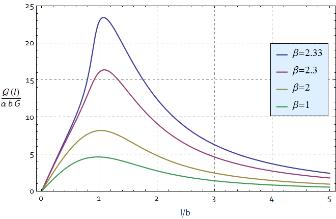
Figure 1: Magnitude of the gravitational force field given by Eqs. (38) and (33) for various values of the parameter $\beta\equiv b^{2}k\alpha$.

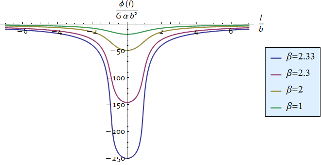
Figure 2: Gravitational potential of the wormhole for the same values of the parameter $\beta\equiv b^{2}k\alpha$ as given in Fig. 1.

Using the expression for the gravitational field, Eq. (38), we can find the gravitational potential using Eq. (34). In Fig. 2 we present the gravitational field for various values of the parameter $\beta$, imposing that when we move away from the wormhole’s throat the gravitational potential goes to zero.

III.4 Pressure support on the wormhole

The results found in the last section allow us to further define the fluid that permeates the Newtonian wormhole. In the case of a static fluid the Euler equation reduces to Eq. (2) and in the wormhole coordinate system is given by

$$\frac{dp}{dl}=-\rho\frac{d\phi}{dl}\,.$$ (40)

Since it is not possible to find a closed form expression for the gravitational field, Eq. (40) can only be solved numerically. The behavior of the fluid’s pressure is then presented in Fig. 3 where it was imposed that at infinity the pressure of the fluid is zero since the density of the fluid, Eq. (29), goes to zero exponentially fast as $l\to\infty$.

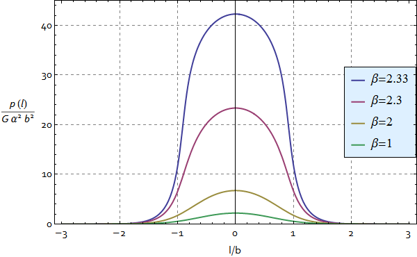
Figure 3: Behavior of the pressure of the fluid that permeates the Newtonian wormhole for the same values of the parameter $\beta\equiv b^{2}k\alpha$ as given in Fig. 1.

Note that the pressure is positive throughout the space. This means that matter gravitates and tends to collapse. However, the negative curvature of space tends to have a repulsive effect on the matter, trying to balance out the gravitational force. There is, however, still the need of a pressure to hold the wormhole against collapse. As is suggested by Fig. 3, from Eqs. (27), (29) and (38) we see that as the value of the parameter $\beta$ approximates its upper bound, Eq. (23), the pressure of the fluid goes to infinity at the throat.

III.5 Test particle dynamics and motion in the wormhole gravitational field

III.5.1 The equations of motion

In the previous section we found the expression for the gravitational field of the Newtonian wormhole, Eq. (38). From this gravitational field we can write the equations of motion for a test particle subjected to the wormhole gravitational field in the wormhole geometry. We use Eq. (4). We start by considering that the particle’s path is described by a curve $c$, whose components $x^{i}$ are given by the parametric equations $x^{i}=\left(l\left(t\right),\theta\left(t\right),\varphi\left(t\right)\right)$. The particle’s generalized velocity $v^{i}\equiv\dot{x}^{i}$, is given by $v^{i}=\left(\dot{l}\left(t\right),\dot{\theta}\left(t\right),\dot{\varphi}\left(t\right)\right)$, where a dot means derivative in relation to time.

The left hand side of Eq. (4) involves the acceleration of the particle, defined as

$$a^{i}=v^{j}\,\nabla_{j}\,v^{i}\,=\dot{v}^{i}+\Gamma_{jk}^{i}v^{j}v^{k}\,,$$ (41)

where the $\Gamma_{jk}^{i}$ are the Christoffel symbols for the Newtonian wormhole metric given in Eq. (27). The right hand side of Eq. (4) is the gravitational field given in Eq. (38). Gathering these results, we are able to write Eq. (4) explicitly.

First, we study the equation for the coordinate $\theta$. Eq. (41) yields $\ddot{\theta}+2\frac{l}{b^{2}+l^{2}}\dot{l}\dot{\theta}-\sin\theta\cos\theta\dot{\varphi}^{2}=0$. If we take the value of $\theta=\pi/2$, then this equation implies that $\dot{\theta}=0$ is a possible solution. Checking that the higher order derivatives are also zero, we conclude that $\theta=\pi/2$ is a consistent solution of the equations of motion.

With this result in hand we can write the equations of motion in a simplified form for the coordinates $l$, $\theta$, and $\varphi$, namely,

$$\ddot{l}+\left[\frac{b\,e^{\frac{l^{2}}{b^{2}}}\left(2b^{2}+l^{2}\right)\left(e+\beta\right)-2\sqrt{b^{2}+l^{2}}\left[\beta\,l^{2}\left(1+l^{2}/b^{2}\right)+b^{2}\left(e^{1+\frac{l^{2}}{b^{2}}}+\beta\right)\right]}{2l\left(b^{2}+l^{2}\right)\left[b\,e^{\frac{l^{2}}{b^{2}}}\left(e+\beta\right)-\sqrt{b^{2}+l^{2}}\left(e^{1+\frac{l^{2}}{b^{2}}}+\beta\right)\right]}\right]\,\,\dot{l}{}^{2}+$$ (42)

$$\hskip 70.2625pt+\left[\frac{b\sqrt{b^{2}+l^{2}}\left(e+\beta\right)-\left(b^{2}+l^{2}\right)\left(e+\beta\,e^{-\frac{l^{2}}{b^{2}}}\right)}{e\,l}\right]\,\,\dot{\varphi}{}^{2}=$$

$$\hskip 70.2625pt=-\frac{G\,m\left(l\right)}{2\sqrt{e}\,\left(b^{2}+l^{2}\right)l}\sqrt{\left(b^{2}+l^{2}\right)\left(e+\beta\,e^{-\frac{l^{2}}{b^{2}}}\right)-b\sqrt{b^{2}+l^{2}}\left(e+\beta\right)}\,,$$

$$\theta=\frac{\pi}{2}\,,\quad\dot{\theta}=0\,,$$ (43)

$$\ddot{\varphi}+2\,\frac{l}{b^{2}+l^{2}}\,\,\dot{l}\,\dot{\varphi}=0\,.$$ (44)

Before trying to solve these equations of motion let us first analyze them.

On the left hand side of Eq. (42), we have two terms that depend on the first derivative of one of the coordinates, one in $\dot{\varphi}^{2}$ and the other in $\dot{l}^{2}$. The former is the usual centripetal force that also arises in classical mechanics in flat space. However the latter term has no flat space counterpart. This term arises indeed from the curvature of space along the radial direction. The curvature, then, implies that a force similar to a centripetal force arises when the particle’s motion has a radial component. Taking the limit $l\to\pm\infty$, and recalling that the wormhole is asymptotically flat, we find that the term in $\dot{l}^{2}$ vanishes, i.e., in flat space it is nonexistent. Still in Eq. (42) one finds that the particle suffers an usual centripetal acceleration $a_{{\rm c}}$ given by

$$a_{{\rm c}}=\left[\frac{b\sqrt{b^{2}+l^{2}}\left(e+\beta\right)-\left(b^{2}+l^{2}\right)\left(e+\beta\,e^{-\frac{l^{2}}{b^{2}}}\right)}{e\,l}\right]\,\dot{\varphi}^{2}\,.$$ (45)

We also see that Eq. (44) can be readily integrated, obtaining

$$h=\left(l^{2}+b^{2}\right)\dot{\varphi}\,,$$ (46)

where $h$ is a constant of integration that can be interpreted as the angular momentum per unit mass of the particle. Thus, angular momentum is conserved as one expects for a central force.

Once the equations of motion of a test particle are found, we have now to solve them. We will study two cases, pure circular motion and a general motion.

III.5.2 Circular motion

Let us first consider the problem of circular motion of a test particle in the Newtonian wormhole background. In this case the radial coordinate $l$ does not change throughout the particle’s motion, therefore, $l=l_{0}$ say, $\dot{l}=0$, and $\ddot{l}=0$. From this, Eq. (42) reduces to

$$\ddot{\varphi}=0\,,$$ (47)

which in turn has a first integral $\dot{\varphi}=\text{\text{constant}}$. With the help of Eq. (42) we can determine this constant and obtain

$$\dot{\varphi}=\sqrt{\frac{\sqrt{e}\,G\,m\left(l_{0}\right)}{2\left(b^{2}+l_{0}^{2}\right)\sqrt{\left(b^{2}+l_{0}^{2}\right)\left(e+\beta\,e^{-\frac{l_{0}^{2}}{b^{2}}}\right)-b\sqrt{b^{2}+l_{0}^{2}}\left(e+\beta\right)}}}\,,$$ (48)

where it is implicit that the particle can rotate in both senses. Equation (48) relates the radial position $l_{0}$ of the particle and the azimuthal velocity $\dot{\varphi}$ that the particle must have in order to describe a circular orbit around the wormhole’s throat. In Fig. 4 we present an example of such circular motion.

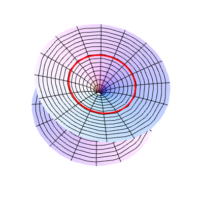
Figure 4: Circular motion of a particle in the Newtonian wormhole for some initial radial position $l_{0}$ and initial angular velocity $\dot{\varphi}$ given by Eq. (48). The wormhole parameters are $b$ and $\alpha$.

This case of circular motion can also be used to check the consistency of our treatment against the analysis presented by Abramowicz et al Abramowicz1 ; Abramowiczellis . Thereby, our purpose is to find the centripetal acceleration using the following expression presented in Abramowiczellis , i.e.,

$$a^{i}=-\frac{v^{2}}{\mathcal{R}}n_{\pm}^{i}\,,$$ (49)

where $v=\sqrt{\left(l^{2}+b^{2}\right)}\dot{\varphi}$ is the modulus of the linear velocity of the particle in circular motion, $n_{\pm}^{i}$ is the outside pointing unit normal to the circle given in Eq. (35), and $\mathcal{R}$ is the the curvature radius of the circle described by the particle’s motion given by Abramowiczellis

$$\mathcal{R}=\tilde{r}\,\left(\frac{dr_{*}}{d\tilde{r}}\right)\,.$$ (50)

Using Eqs. (31) and (32) for the geodesic radius $r_{*}$, and the circumferential radius $\tilde{r}$, respectively, we find that in this case the curvature radius is given by

$$\mathcal{R}=\sqrt{\frac{\left(b^{2}+l^{2}\right)^{2}e}{\left(b^{2}+l^{2}\right)\left(e+\beta\,e^{-\frac{l^{2}}{b^{2}}}\right)-b\sqrt{b^{2}+l^{2}}\left(e+\beta\right)}}\,.$$ (51)

Gathering all the intermediate results, and putting the centripetal acceleration $a_{c}$ as $a_{{\rm c}}=a^{l}$, we can write Eq. (49) explicitly has

$$a_{{\rm c}}=\left[\frac{b\sqrt{b^{2}+l^{2}}\left(e+\beta\right)-\left(b^{2}+l^{2}\right)\left(e+\beta\,e^{-\frac{l^{2}}{b^{2}}}\right)}{e\,l}\right]\,\dot{\varphi}^{2}\,,$$ (52)

which is exactly the expression that we found for the centripetal acceleration that appears in Eq. (45).

III.5.3 General motion

Aside the case of circular motion which can be treated analytically, we can use numerical methods to solve the equations (42)-(44) to study a more generic motion of a particle on the Newtonian wormhole given its initial position and velocity. We present in Fig. 5 some graphical solutions of Eqs. (42)-(44) for general motions.

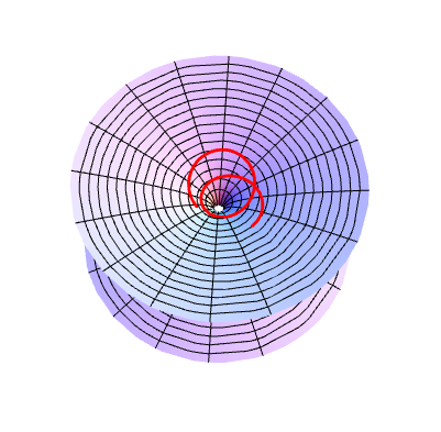
(a)

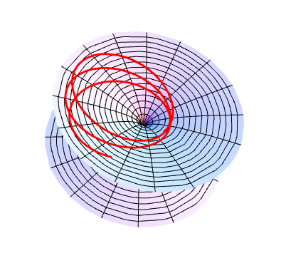
(b)

Figure 5: Panel (a): Particle’s motion in the wormhole background for a relatively small initial angular velocity $\dot{\varphi}$. Panel (b): Particle’s motion in the wormhole background for a relatively large angular velocity $\dot{\varphi}$. In all figures the particle’s initial radial position is taken to be at some $l_{0}$, and the initial radial velocity $\dot{l}_{0}$ is zero. The wormhole parameters are $b$ and $\alpha$.

IV The limiting case: Are there Newtonian black holes?

Figs. 1 and 2 suggest that as the parameter $\beta$ approaches the upper bound given by Eq. (23) the value of the gravitational field $\mathcal{G}^{i}\left(l\right)$ and the gravitational potential itself have a somewhat weird behavior. Indeed, analyzing Eqs. (38) and (39), one finds that, for some value $l_{{\rm h}}$ of the radial coordinate $l$, the gravitational field $\mathcal{G}^{i}\left(l\right)$ goes to infinity when the value of the parameter $\beta$ approaches the value $\beta_{{\rm crit}}$, given by Eq. (23).

This is a very surprising behavior since the system somehow develops a Newtonian event horizon, in the sense that for $\beta=\beta_{{\rm crit}}$ every test particle that crosses the sphere defined by $l=l_{{\rm h}}$ can only return back from that inner sphere to the outside if it has infinite acceleration, and thus an infinite velocity. Hence, an observer beyond that sphere can never affect an outside observer. It characterizes a Newtonian black hole.

However, note also that as the value of the parameter $\beta$ approximates its upper bound, Eq. (23), the fluid pressure goes to infinity at the throat, see also Fig. 3. Thus, the black hole cannot be sustained with this type of matter at such an extreme situation. Presumably at such $\beta_{{\rm crit}}$, the matter collapses leaving behind two disjoint regions in each side of the original space with a singularity at the center where the density and the space curvature blow up. This final singularity formed from the collapse of the original matter could also be considered a Newtonian black hole in this enhanced Newtonian gravitation, since only test particles with infinite velocities could escape from it.

V Conclusions

We have presented a Newtonian wormhole in Newtonian gravitation in curved space, enhanced with relation between the curvature and the matter density. The wormhole is spherically symmetric having two connected asymptotic flat regions. The wormhole’s mass density is positive throughout the space. This is distinct from wormholes in general relativity where the flare out condition imposes some form of exoticity for the matter. The wormhole is hold against collapse by pressure. Test particle motion in the wormhole gravitational field have shown that the three distinct dynamical radii, namely, the geodesic, circumferential, and curvature radii, appear naturally in the study of circular motion. A limiting case, when the parameter $\beta$ satisfies $\beta=\beta_{\rm crit}$, suggests the possibility of having a Newtonian black hole in a region of finite size.

Appendix I: Spatial Geodesics

Here we display the spatial geodesics of the wormhole space.

V.1 Spatial geodesic equations

To complete the analysis of the Newtonian wormhole geometry, we find the expressions for the geodesics in this space. To start we consider a spatial curve $c$ on the Newtonian wormhole parametrized by a parameter $\lambda$. A point on $c$ is given by the parametric equation $c^{i}\left(\lambda\right)=\left(l\left(\lambda\right),\theta\left(\lambda\right),\varphi\left(\lambda\right)\right)$ and the tangent vector to the curve at a given point by $c^{i}\,{}^{\prime}\left(\lambda\right)=\left(l^{\prime}\left(\lambda\right),\theta^{\prime}\left(\lambda\right),\varphi^{\prime}\left(\lambda\right)\right)$, where a dash means derivative with respect to the affine parameter $\lambda$. The curve $c^{i}$ is said to be a geodesic if it parallel transports its tangent vector along itself, i.e., its tangent vector must be such that the equation

$$c^{i}\,{}^{\prime}\nabla_{i}\,c\,^{j}\,{}^{\prime}=0\,,$$ (53)

is verified, and where $\nabla$ is the covariant derivative. Before we write the geodesic equations explicitly for this space, we can simplify the calculations by noticing that due to the spherical symmetry of the space we can always choose a coordinate system in such a way that the polar angle, represented by the coordinate $\theta$, is constant along the curve and equal to $\pi/2$. In other words, since the $2$-sphere, $S^{2}$, is a submanifold of the space and it is a well known fact that part of great circles are geodesics in $S^{2}$, then any geodesic on the space, under isometries, is part of a great circle. Thus, the geodesic equations for the wormhole space are

$$\left\{\begin{aligned} &l^{\prime\prime}+\left[\frac{b\,e^{\frac{l^{2}}{b^{2}}}\left(2b^{2}+l^{2}\right)\left(e+\beta\right)-2\sqrt{b^{2}+l^{2}}\left[\beta\,l^{2}\left(1+l^{2}/b^{2}\right)+b^{2}\left(e^{1+\frac{l^{2}}{b^{2}}}+\beta\right)\right]}{2l\left(b^{2}+l^{2}\right)\left[b\,e^{\frac{l^{2}}{b^{2}}}\left(e+\beta\right)-\sqrt{b^{2}+l^{2}}\left(e^{1+\frac{l^{2}}{b^{2}}}+\beta\right)\right]}\right]\,\,l^{\prime 2}+\\ &\hskip 135.15059pt+\left[\frac{b\sqrt{b^{2}+l^{2}}\left(e+\beta\right)-\left(b^{2}+l^{2}\right)\left(e+\beta\,e^{-\frac{l^{2}}{b^{2}}}\right)}{e\,l}\right]\,\,\varphi^{\prime 2}=0\,;\\ &\varphi^{\prime\prime}+2\frac{l}{b^{2}+l^{2}}\,l^{\prime}\varphi^{\prime}=0\,;\\ &\theta^{\prime}=0\,,\\ &\theta=\pi/2\,.\end{aligned}\right.$$ (54)

The geodesic equations in their general form are quite complicated to solve and find an analytical solution. We can however consider simpler cases than the general one.

V.2 Spatial azimuthal geodesics

Let us first consider the case of purely azimuthal geodesics, i.e., consider geodesics of the form $c^{i}\left(\lambda\right)=\left(l_{0},\pi/2,\varphi\left(\lambda\right)\right)$. In this case, the geodesic equations simplify to $\varphi^{\prime\prime}=0$. If we take the initial and final position of the geodesic to be, respectively, $c^{i}\left(0\right)=\left(l_{0},\pi/2,\varphi_{0}\right)$ and $c^{i}\left(\lambda_{f}\right)=\left(l_{0},\pi/2,\varphi_{f}\right)$ we conclude that

$$\varphi\left(\lambda\right)=\frac{\varphi_{f}-\varphi_{0}}{\lambda_{f}}\,\lambda+\varphi_{0}\,.$$ (55)

V.3 Spatial radial geodesics

Let us now consider the case of purely radial geodesics. In this case the geodesics are of the form $c^{i}\left(\lambda\right)=\left(l\left(\lambda\right),\pi/2,\varphi_{0}\right)$, such that the geodesic equations simplify to

$$l^{\prime\prime}+\left[\frac{b\,e^{\frac{l^{2}}{b^{2}}}\left(2b^{2}+l^{2}\right)\left(e+\beta\right)-2\sqrt{b^{2}+l^{2}}\left[\beta\,l^{2}\left(1+l^{2}/b^{2}\right)+b^{2}\left(e^{1+\frac{l^{2}}{b^{2}}}+\beta\right)\right]}{2l\left(b^{2}+l^{2}\right)\left[b\,e^{\frac{l^{2}}{b^{2}}}\left(e+\beta\right)-\sqrt{b^{2}+l^{2}}\left(e^{1+\frac{l^{2}}{b^{2}}}+\beta\right)\right]}\right]\,\,l^{\prime 2}=0\,.$$ (56)

This equation is still too complicated and it does not seem to be possible to find an analytical solution to it. We can, however, consider a further simplification, namely, we consider that the initial and final radial coordinate, $l_{0}$ and $l_{f}$, respectively, are very close to the wormhole’s throat. This allow us to Taylor expand the expression in parenthesis in Eq. (56) such that

$$l^{\prime\prime}+\left[\frac{l\left(e-3\beta\right)}{4b^{2}\left(\beta-e\right)}\right]\,\,l^{\prime 2}=0\,.$$ (57)

This expression can be analytically integrated. If we then consider the initial and final points to be $c^{i}\left(0\right)=\left(l_{0},\pi/2,\varphi_{0}\right)$ and $c^{i}\left(\lambda_{f}\right)=\left(l_{f},\pi/2,\varphi_{0}\right)$, respectively, we find that

$$l\left(\lambda\right) =-i\sqrt{\frac{8b^{2}\left(\beta-e\right)}{e-3\beta}}\text{erf}^{-1}\left(i\,\frac{\lambda_{f}-\lambda}{\lambda_{f}}\text{erfi}\left(\sqrt{\frac{e-3\beta}{8b^{2}\left(\beta-e\right)}}\,l_{0}\right)+\right.$$ (58)

$$\left.\hskip 160.59999pt+\frac{i\,\lambda}{\lambda_{f}}\text{erfi}\left(\sqrt{\frac{e-3\beta}{8b^{2}\left(\beta-e\right)}}\,l_{f}\right)\right)$$

where $\text{erf}^{-1}$ represents the inverse Gauss error function and erfi the imaginary Gauss error function. Equation (58) gives the expression for the radial coordinate of purely radial geodesics when the two considered points are very close to the wormhole’s throat.

V.4 Spatial general geodesics

The simplifications adopted in the previous subsections greatly simplified the geodesic equations and allowed us to find closed form solutions for those simplified cases. Let us, however, tackle the general problem of studying geodesics of the form $c^{i}\left(\lambda\right)=\left(l\left(\lambda\right),\pi/2,\varphi\left(\lambda\right)\right)$, with initial and final points $c^{i}\left(0\right)=\left(l_{0},\pi/2,\varphi_{0}\right)$ and $c^{i}\left(\lambda_{f}\right)=\left(l_{f},\pi/2,\varphi_{f}\right)$, respectively. Notice that we imposed the angular coordinate $\theta=\pi/2$. This reflects the argument that we presented in the beginning of this section, i.e., given any two points on the spherically symmetric Newtonian wormhole we can always find an isometry such that the geodesic that connects those two points is part of a great circle.

To start, we introduce a new equation:

$$l^{\prime 2}\left(\frac{e\,l^{2}}{\left(b^{2}+l^{2}\right)\left(e+\beta\,e^{-\frac{l^{2}}{b^{2}}}\right)-b\sqrt{b^{2}+l^{2}}\left(e+\beta\right)}\right)+\varphi^{\prime 2}\left(b^{2}+l^{2}\right)=1\,.$$ (59)

This equation represents the restriction that the norm of the tangent vector to the curve $c^{i}$ is constant, which we normalized and set to $1$. Next, we integrate the azimuthal equation in Eq. (54), obtaining

$$\varphi^{\prime}=\frac{C}{b^{2}+l^{2}}\,,$$ (60)

where $C$ is a constant of integration. Substituting Eq. (60) in Eq. (59) we find that

$$l^{\prime}=\sqrt{\left[\frac{e+\beta\,e^{-\frac{l^{2}}{b^{2}}}}{e\,l^{2}}-\frac{b\left(e+\beta\right)}{e\,l^{2}\sqrt{b^{2}+l^{2}}}\right]\left(l^{2}+b^{2}-C^{2}\right)}\,.$$ (61)

Dividing Eq. (60) by Eq. (61) we finally find that

$$\frac{d\varphi}{dl}=C\sqrt{\frac{e\,l^{2}}{\left[\left(b^{2}+l^{2}\right)^{2}\left(e+\beta\,e^{-\frac{l^{2}}{b^{2}}}\right)-b\sqrt{\left(b^{2}+l^{2}\right)^{3}}\left(e+\beta\right)\right]\left(l^{2}+b^{2}-C^{2}\right)}}\,,$$ (62)

or

$$\varphi\left(l_{f}\right)={\displaystyle C\int_{l_{i}}^{l_{f}}\sqrt{\frac{e\,l^{2}}{\left[\left(b^{2}+l^{2}\right)^{2}\left(e+\beta\,e^{-\frac{l^{2}}{b^{2}}}\right)-b\sqrt{\left(b^{2}+l^{2}\right)^{3}}\left(e+\beta\right)\right]\left(l^{2}+b^{2}-C^{2}\right)}}}\,\,dl+\varphi_{0}\,,$$ (63)

which can be numerical integrated, provided the value of the constant $C$ is given, such that the geodesic’s path is described by $c(l)=\left(l,\pi/2,\varphi(l)\right)$.

We can further define the constant of integration $C$. Let’s consider the unit vector

$$X_{\varphi}^{i}=\frac{1}{\sqrt{b^{2}+l^{2}}}\delta_{\varphi}^{i}\,,$$ (64)

defined has the tangent unit vector to curves with constant $l$ and $\theta$ coordinates. Taking the dot product of $X_{\varphi}^{i}$ and the tangent vector of the geodesic $c^{i}\,{}^{\prime}$, we have, using Eq. (27), that

$$X_{\varphi}^{i}\,c_{i}\,^{\prime}=\sqrt{\left(b^{2}+l^{2}\right)}\varphi^{\prime}=\frac{C}{\sqrt{b^{2}+l^{2}}}\,,$$ (65)

where in the last step we used Eq. (60). By other hand, defining the smaller angle between $X_{\varphi}^{i}$ and $c^{i}\,{}^{\prime}$ as $\xi$, the definition of the dot product implies that

$$X_{\varphi}^{i}\,c_{i}\,^{\prime}=\cos\left(\xi\right)\,,$$ (66)

where we used the fact that the vectors $X_{\varphi}^{i}$ and $c^{i}\,{}^{\prime}$ are unitary vectors. Comparing Eqs. (65) and (66) we find that the integration constant $C$ is related to the angle $\xi$ by:

$$C=\sqrt{b^{2}+l^{2}}\cos\left(\xi\right)\,.$$ (67)

Incidentally, Eqs. (63) and (67) allow us to further describe the purely radial geodesics, studied in the previous subsection where a closed form solution for such geodesics was only possible if the beginning and ending points were very close to the wormhole’s throat. If we consider that the angle $\xi=\pi/2$ in Eq. (67), using Eq. (63) we find that the coordinate $\varphi\left(l\right)$ is constant along the geodesic. This is exactly as we expected since for $\xi=\pi/2$ the geodesic $c^{i}$ is orthogonal to the geodesics with constant $l$-coordinate, i,e,, $c^{i}$ is a radial geodesic. This result allow us to describe all the radial geodesics on the wormhole space, such that, $c^{i}\left(l\right)=\left(l,\pi/2,\varphi_{0}\right)$, supplanting Eq. (58) which was valid only when the initial and final points were very close to the wormhole’s throat.

References

- (1) M. Abramowicz, “The perihelion of Mercury advance calculated in Newton’s theory”, arXiv:1212.0264 [astro-ph.EP] (2012).
- (2) M. Abramowicz, G. F. R. Ellis, J. Horak, and M. Wielgus, “The perihelion of Mercury advance and the light bending calculated in (enhanced) Newton’s theory”, Gen. Relativ. Gravit 46, 1630 (2014); arXiv:1303.5453 [gr-qc] (2013).
- (3) J. Ehlers, “Contributions to the relativistic mechanics of continuous media”, Gen. Relativ. Gravit 25, 1225 (1993), (translation of the Proceedings of the Mathematical-Natural Science Section of the Mainz Academy of Science and Literature 11, 792 (1961)).
- (4) G. F. R. Ellis and H. van Elst, “Cosmological models”, in Proceedings of the NATO Advanced Study Institute on Theoretical and Observational Cosmology, Cargèse, NATO Science Series, Series C, Mathematical and Physical Sciences 541, 1, ed. M. Lachièze-Rey (Kluwer Academic, Boston 1999); arXiv:gr-qc/9812046.
- (5) N. Dadhich, “A novel derivation of the rotating black hole metric”, Gen. Relativ. Gravit. 45, 2383 (2013); arXiv:1301.5314 [gr-qc].
- (6) C. DeWitt and B. S. DeWitt (eds.), Black holes, Proceedings of the 1972 Les Houches Summer School (Gordon and Breach, New York, 1973).
- (7) W. Israel, “Dark stars: the evolution of an idea”, eds. S. W. Hawking and W. Israel, W., Three Hundred Years of Gravitation (Cambridge University Press, Cambridge, 1987) p. 199.
- (8) S. Chandrasekhar, “The maximum mass of ideal white dwarfs”, Astrophys. J., 74, 81 (1931).
- (9) S. Chandrasekhar, An introduction to the study of stellar structure (The University of Chicago Press, 1st edition, Chicago, 1939), (republished by Dover, New York, 1958).
- (10) R. Penrose, “Gravitational collapse: A review”, in Physics and Astrophysics of Neutron Stars and Black Holes, LXV Corso, eds. R. Giacconi and R. Ruffini (Soc. Italiana di Fisica, Bologna, 1978), p. 566.
- (11) G. C. McVittie, “Laplace’s alleged “black hole””, The Observatory 98, 272 (1978).
- (12) J. Eisenstaedt, “Dark body and black hole horizons”, Gen. Relativ. Gravit. 23, 75 (1991).
- (13) A. K. Raychaudhuri, “Black holes and Newtonian physics”, Gen. Relativ. Gravit. 24, 75 (1992).
- (14) G. Preti, “Schwarzschild radius before general relativity: Why does Michell-Laplace argument provide the correct answer?”, Found. Phys. 39, 1046 (2009).
- (15) B. Paczyński and P. J. Wiita, “Thin accretion disks and supercitical luminosities”, Astron. and Astroph 88, 23 (1980).
- (16) M. A. Abramowicz, B. Czerny, J. P. Lasota, and E. Szuszkiewicz, “Slim accretion disks”, Astrophys. Journ. 332, 646 (1988).
- (17) M. S. Morris, and K. S. Thorne, “Wormholes in spacetime and their use for insterstellar travel: A tool for teaching general relativity”, Am. J. Phys. 56, 395 (1988).
- (18) M. Visser, Lorentzian wormholes: From Einstein to Hawking (AIP Press, American Institute of Physics, 1995).
- (19) D. Hochberg and M. Visser, “Geometric structure of the generic static traversable wormhole throat”, Phys. Rev. D 56, 4745 (1997); arXiv:gr-qc/9704082.
- (20) M. Visser, Sayan Kar, and N. Dadhich, “Traversable wormholes with arbitrarily small energy condition violations”, Phys. Rev. Lett. 90, 064004 (2003); arXiv:gr-qc/0302049.
- (21) J. P. S. Lemos, F. S. N. Lobo, and S. Q. Oliveira, “Morris-Thorne wormholes with a cosmological constant”, Phys. Rev. D 68, 064004 (2003); arXiv:gr-qc/0302049.
- (22) O. B. Zaslavskii, “Exactly solvable model of wormhole supported by phantom energy”, Phys. Rev. D 72, 061303 (2005); arXiv:gr-qc/0508057.
- (23) M. Thibeault, C. Simeone, and E. F. Eiroa, “Thin-shell wormholes in Einstein-Maxwell theory with a Gauss-Bonnet term”, Gen. Relativ. Gravit. 38, 1593 (2006); arXiv:gr-qc/0512029 [gr-qc].
- (24) P. K. F. Kuhfittig, “A single model of traversable wormholes supported by generalized phantom energy or Chaplygin gas”, Gen. Relativ. Gravit. 41, 1485 (2009); arXiv:0904.3566 [gr-qc].
- (25) A. A. Usmani, F. Rahaman, S. Ray, S. A. Rakib, Z. Hasan, and P. K. F. Kuhfittig, “Thin-shell wormholes from charged black holes in generalized dilaton-axion gravity”, Gen. Relativ. Gravit. 42, 2901 (2010); arXiv:1001.1415 [gr-qc].
- (26) A. B. Balakin, J. P. S. Lemos, and A. E. Zayats, “Nonminimal coupling for the gravitational and electromagnetic fields: Traversable electric wormholes”, Phys. Rev. D 81, 084015 (2010); arXiv:1003.4584 [gr-qc].
- (27) G. A. S. Dias and J. P. S. Lemos, “Thin-shell wormholes in d-dimensional general relativity: Solutions, properties, and stability’, Phys. Rev. D 82, 084023 (2010); arXiv:1008.3376 [gr-qc].
- (28) K. A. Bronnikov, R. A. Konoplya, and A. Zhidenko, “Instabilities of wormholes and regular black holes supported by a phantom scalar field”, Phys. Rev. D 86, 024028 (2009); arXiv:1205.2224 [gr-qc].
- (29) V. Diemer and E. Smolarek, “Dynamics of test particles in thin-shell wormhole spacetimes”, Class. Quantum Grav. 30, 175014 (2012); arXiv:1302.1705 [gr-qc].
- (30) M. Halilsoy, A. Ovgun, and S. H. Mazharimousavi, “Thin-shell wormholes from the regular Hayward black hole”, Eur. Phys. J. C 74, 2796 (2013); arXiv:1312.6665 [gr-qc].
- (31) V. Dzhunushaliev, V. Folomeev, B. Kleihaus, and J. Kunz, “Hiding a neutron star inside a wormhole”, Phys. Rev. D 89, 084018 (2014); arXiv:1401.7093 [gr-qc].
- (32) L. M. Butcher, “Casimir energy of a long wormhole throat”, Phys. Rev. D 90, 024019 (2014); arXiv:1405.1283 [gr-qc].