Analyzing long-term correlated stochastic processes by means of recurrence networks: Potentials and pitfalls

Abstract

Long-range correlated processes are ubiquitous, ranging from climate variables to financial time series. One paradigmatic example for such processes is fractional Brownian motion (fBm). In this work, we highlight the potentials and conceptual as well as practical limitations when applying the recently proposed recurrence network (RN) approach to fBm and related stochastic processes. In particular, we demonstrate that the results of a previous application of RN analysis to fBm (Liu et al., Phys. Rev. E 89, 032814 (2014)) are mainly due to an inappropriate treatment disregarding the intrinsic non-stationarity of such processes. Complementarily, we analyze some RN properties of the closely related stationary fractional Gaussian noise (fGn) processes and find that the resulting network properties are well-defined and behave as one would expect from basic conceptual considerations. Our results demonstrate that RN analysis can indeed provide meaningful results for stationary stochastic processes, given a proper selection of its intrinsic methodological parameters, whereas it is prone to fail to uniquely retrieve RN properties for non-stationary stochastic processes like fBm.

I Introduction

Many tools of nonlinear time series analysis are based on the theory of (deterministic) dynamical systems Kantz and Schreiber (2004); Sprott (2003), i.e., the time evolution of the system under study is considered in some phase space spanned by the relevant dynamical variables. Among others, the recurrence of previous states in phase space Poincaré (1890) is a particular fundamental property of dynamical systems with a finite phase space volume (e.g., attractors of a dissipative system, Hamiltonian systems with a bound phase space, or even stationary stochastic systems in finite time). The concept of recurrence implies that the dynamics of a system returns to an arbitrarily small neighborhood of any of its previously assumed states within a finite (but possibly large) amount of time. For deterministic-chaotic systems, this is guaranteed by the invariance of the set which forms the support of the attractor Ott (2002); Sprott (2003).

Recently, complex network representations have been proposed to characterize statistical properties of the underlying system associated with its geometry in phase space Xu et al. (2008); Marwan et al. (2009); Donner et al. (2010a). For this purpose, a proper transformation from the set of state vectors in phase space to a complex network representation is required. In this work, we focus on the recurrence network (RN) approach, the vertices of the network are given by the individual state vectors sampled from a given trajectory, whereas network connectivity is established according to their mutual closeness in phase space (i.e., whether or not their mutual distance is smaller than a pre-defined threshold $\varepsilon$). Mathematically, given two state vectors $\mathbf{x}_{i}$ and $\mathbf{x}_{j}$ (where $i$ and $j$ denote time indices associated with two possibly different points $t_{i}$ and $t_{j}$ in time), the adjacency matrix $A_{i,j}$ of the RN is defined as

$$A_{i,j}(\varepsilon)=\Theta(\varepsilon-\|\mathbf{x}_{i}-\mathbf{x}_{j}\|)-\delta_{i,j},$$ (1)

where $\Theta(\cdot)$ is the Heaviside “function”, $\varepsilon$ is the prescribed maximum distance, $\|\cdot\|$ a norm in phase space (e.g., Euclidean, Manhattan, or maximum norm), and $\delta_{i,j}$ is the Kronecker delta. RN analysis originates from the recurrence plot concept Marwan et al. (2007); Eckmann et al. (1987) and its basic assumption is, as the term indicates, the unambiguous presence of recurrence behavior.

Stationarity is a condition required by most tools of both linear and nonlinear time series analysis Kantz and Schreiber (2004), including the RN approach. A signal is (strongly) stationary if all joint probabilities of finding the system at some time in one state and at some later time in another state are independent of time within the observation period. The minimal requirement for most approaches is weak stationarity, that is, mean and variance of the underlying process are constant and the auto-covariances depend only on the time lag.

In turn, many real-world processes are non-stationary. For instance, climate or hydrological data often show seasonal variations. Economic and financial time series typically exhibit (irregular) cycles of all orders of magnitude. Non-stationary behaviors can be expressed in terms of trends, cycles, random walks, or combinations of the latter three. Often, long-range dependence and self-similarity are involved. One classical example of a class of such non-stationary processes is fractional Brownian motion (fBm), which has long-range temporal correlations as its defining property Mandelbrot and Van Ness (1968). Specifically, for an fBm process $\{X_{t}\}$, the variance scales as $\sigma_{X_{t}}^{2}\propto t^{2H}$ (i.e., non-stationarity in variance). The long range of the process is characterized by the Hurst exponent $H$ when positively correlated (persistence) for $1/2<H<1$, while suppressed (anti-persistence) for $0<H<1/2$. $H=1/2$ corresponds to the classical Brownian motion.

Non-stationarity provides a great challenge to both linear and nonlinear time series analysis, including complex network approaches to analyze time series data. There are some methods that are specifically tailored to cope with non-stationarity. Among others, detrended fluctuation analysis (DFA) Peng et al. (1994); Kantelhardt et al. (2001); Hu et al. (2001) and related techniques have been widely used for estimating the Hurst exponent from non-stationary model data as well as real-world applications from various fields (e.g., Bunde and Havlin (2002); Kantelhardt et al. (2003)). In contrast, regarding the RN approach, non-stationarity due to time-dependent system parameters can cause a systematic loss of recurrences. Anyway, RNs have been recently proposed to characterize fBm Liu et al. (2014). Notably, the results of the latter study have been obtained only numerically and not explained theoretically so far. However, as we will demonstrate in the course of this work, they have rather limited physical interpretation. More generally, we will discuss how spurious results and pitfalls of RN analysis may be produced when this method is inappropriately applied to study fBm or other non-stationary stochastic processes, and that the results of Liu et al. (2014) are mainly of such spurious nature.

This paper is organized as follows: In Section II, we discuss the construction of RNs from non-stationary fBm data. We demonstrate that it is not possible to define generally applicable embedding parameters as required for a systematic investigation of the potential effect of $H$ on the RN properties. Specifically, we provide numerical evidence that the latter properties (for given embedding parameters) depend explicitly on the system size, which generally does not apply to stationary systems provided that the sample size is large enough and sampling artifacts as well as transient behavior are avoided. Subsequently, in Section III, we turn to the RN properties of the closely related fractional Gaussian noise (fGn), the incremental process associated with fBm, which is stationary. For the latter, the dependence of the network characteristics on $H$ is – in contrast to fBm – well-behaved. However, the considered embedding dimension still plays an important role when characterizing the RN structures. All results are summarized and further discussed in Section IV.

II RN analysis of fBm processes

The application of RNs to the analysis of nonlinear time series implicitly assumes the validity of two fundamental assumptions: (i) the intrinsic model parameters and statistical characteristics of the system remain constant over time and (ii) the system under study is sufficiently sampled (i.e., time resolution and time series length are sufficient to approximate the system). The first assumption is equivalent to the condition of stationarity, while the second one mainly requires a proper coverage of phase space by a suitably embedded time series. Both requirements are consequences of the fact that we approach the system’s dynamics by a single finite time series, which is common to time series analysis problems. Note that there have been attempts to characterize non-stationary systems by means of RN analysis using sliding windows approaches, which have provided interesting results regarding the presence of bifurcation or other qualitative changes in the dynamical regime Donges et al. (2011a, b). However, these considerations have been related to systems with supposed time-varying parameters rather than non-stationary stochastic systems where the parameters are constant. Therefore, this approach might not be helpful in the present context dealing with non-stationary variance.

In the following, we will focus on two important algorithmic parameters of the RN approach, embedding dimension and delay. The impact of other parameters such as recurrence threshold $\varepsilon$, sampling rate, or even the selection of variables in multi-dimensional systems has been extensively discussed elsewhere Donner et al. (2010b); Strozzi et al. (2011) for deterministic systems, but not yet for stochastic ones. For the sake of brevity, we present only a brief corresponding discussion here. Specifically, since we consider discrete-time univariate stochastic processes, only $\varepsilon$ is relevant, but can be treated mostly alongside the theoretical considerations presented in Donges et al. (2012).

By means of conceptual considerations as well as numerical experiments, in the remainder of this section, we will address the following three questions: (i) Can we use embedding techniques for fBm (or, more generally, non-stationary stochastic processes)? (ii) What are the intrinsic limitations of this approach? (iii) Which implications do these limitations have for RN analysis?

II.1 Time-delay embedding: Theoretical considerations

As the most prominent subject of recent studies involving RN analysis Marwan et al. (2009); Donner et al. (2010a, 2011a); Zou et al. (2010, 2012a), chaotic attractors exhibit some complex geometric structure in their respective phase space, motivating the term “strange attractors”. Typically, this structure is associated with self-similar (fractal) characteristics. (Notably, there are examples for strange non-chaotic attractors as well Grebogi et al. (1984); Feudel et al. (2006).) Strange attractors emerge in deterministic dynamical systems, and the resulting asymptotic set of state vectors approached by the system forms some finite object in phase space. The dynamical properties of the system and the geometric characteristics of the attractor are commonly closely interrelated Sprott (2003); Donner et al. (2011b).

Taking this idea further, it is a natural approach to describe dynamical systems of whatever kind by a geometric object in some appropriately defined phase space. This is the basis of RN analysis, which takes the existence of such a phase space (at least in an abstract sense) as a fundamental requirement. Given this fact, RN analysis may be applied if the available data series provides enough information to describe (or approximate) the geometric structure of the sampled trajectory sufficiently. Specifically, transient dynamics has to be excluded, data length and sampling frequency need to be appropriate, and the data object in phase space needs to be dynamically invariant or at least bound in phase space with stationary properties.

Given a scalar time series $\{x_{i}\}$ ($i=1,\dots,N$), in order to apply RN analysis we first have to convert the data into state vectors in some appropriately reconstructed phase space. A common method from dynamical systems theory to define such a phase space is time-delay embedding Takens (1981). In fact, the concept of a phase space representation rather than a “simple” time or frequency domain approach is the hallmark of many methods of nonlinear time series analysis, requiring embedding as the first step. Here, we define $\mathbf{x}_{i}=(x_{i},x_{i-\tau},\cdots,x_{i-(m-1)\tau})$ to obtain an $m$-dimensional time-delay embedding of $x_{i}$ with embedding delay $\tau$ for obtaining state vectors in phase space Takens (1981). It has been proven that for deterministic dynamical systems, the thus reconstructed phase space is topologically equivalent to the original space if $m>2D_{F}$, where $D_{F}$ is the fractal dimension of the support of the invariant measure generated by the dynamics in the true (but often at most partially observed) state space. Note that $D_{F}$ can be much smaller than the dimension of the underlying original (physical) phase space spanned by all relevant system variables.

From a practical perspective, when analyzing a scalar time series of whatever origin, neither embedding dimension $m$ nor delay $\tau$ are known a priori. The false nearest-neighbors (FNN) method Kennel et al. (1992) was introduced to derive a reasonable guess of how to choose $m$ based on studying whether or not proximity relations between state vectors are lost when the embedding dimension is successively increased. If a reasonable embedding dimension is found, all dynamically relevant coordinates of the system are appropriately represented, so that all proximity relationships are correct and not due to lower-dimensional projection effects. In a similar spirit, the first root of the auto-correlation function (ACF) of a time series often yields a good estimate for $\tau$. A more refined method is to use time-delayed mutual information Fraser and Swinney (1986).

While the aforementioned approaches to determining $m$ and $\tau$ commonly work well for data from deterministic dynamical systems, applying them to fBm leads to severe conceptual problems:

On the one hand, we note that the concepts of a fractal dimension has two aspects when being applied to a stochastic process instead of a deterministic dynamical system. From the phase space perspective, the fractal dimension is commonly defined as some scaling property described by a parameter that converges to a fixed value as $N\to\infty$ and $m$ is sufficiently high. This fact is used, for example, in the famous Grassberger-Procaccia algorithm for estimating the correlation dimension $D_{2}$ of chaotic attractors Grassberger and Procaccia (1983). However, according to the latter viewpoint, stochastic behavior is characterized by an absence of such convergence, formally leading to $D_{2}=\infty$. Finite estimates of $D_{2}$ are spurious due to the finite amount of data used. The latter result is reasonable since an infinite amount of data (i.e., the innovations at each time step) are necessary to fully describe the evolution of a stochastic process.

As an alternative perspective, the fractal dimension of a stochastic process is often defined via the fractal dimension of its graph. For a one-dimensional process, this graph is represented in the $(t,x)$-plane, and its dimension is hence bound from above by $D_{G}=2$. Specifically, for fBm with a Hurst exponent $H\in(0,1)$, it has been shown that $D_{G}=2-H$, taking the different scaling behavior in association with the process’ self-similarity into account Mandelbrot (1982); Gneiting and Schlather (2004). However, the latter aspect is clearly distinct from the notion of fractal dimensions used in the phase space context. Thus, from a conceptual perspective, the embedding dimension should be chosen infinitely large. In turn, finite $m$ will necessarily cause spurious results since the full complexity of the system’s (discrete) trajectory is not captured.

On the other hand, the embedding delay $\tau$ is not considered in the mathematical embedding theorems for deterministic dynamical systems. Embeddings with the same embedding dimension $m$ but different $\tau$ are topologically equivalent in the mathematical sense Kantz and Schreiber (2004), but in reality a good choice of $\tau$ facilitates further analysis. If $\tau$ is small compared to the relevant internal time-scales of the system, successive elements of the delay vectors are strongly correlated. This leads to the practical requirement that the embedding delay should cover a much longer time interval than the largest characteristic time-scale that is relevant for the dynamics of the system. However, in fBm arbitrarily long time-scales are relevant due to the self-similar nature of the process. This makes finding a feasible value of $\tau$ a challenging (and, regarding formal optimality criteria, even theoretically impossible) task.

In summary, we emphasize that in the case of non-stationary fBm, the fundamental concepts of phase space reconstruction and low-dimensional dynamics do not apply (not even approximately) anymore. Therefore, any attempt to applying RN analysis to fBm directly necessarily yields results that hold only for the particular embedding parameters chosen and the specific length of the given time series Liu et al. (2014). We will demonstrate some numerical results illustrating these points in more detail in the following.

II.2 Numerical results

Estimating the ACF of a stationary time series at lag $\tau$ is straightforward as long as $\tau$ is small compared to the total length of the time series, $N$. For stationary stochastic processes, the functional form and rate of decay of the ACF depends on the specific properties of the process. Specifically, for a stationary long-range correlated process, the ACF decays like a power-law with the characteristic exponent being directly related with $H$ Witt and Malamud (2013).

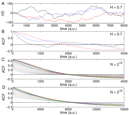
Figure 1: (A) Three example trajectories of fBm with $H=0.7$ and (B) the corresponding ACFs. (C) Average ACFs taken over 200 independent realizations of fBm with the same Hurst exponent $H$. Different line colors correspond to different values of $H$ from $0.05$ to $0.95$ in steps of $0.05$ (from bottom to top at small $\tau$). In all cases, the time series length has been set to $N=2^{13}$. (D) As (C) for $N=2^{15}$.

In contrast to this, for the non-stationary fBm sample estimates of the ACF decay extremely slowly beyond the “normal” behavior of stationary long-range dependent processes, which can be seen clearly in Fig. 1 (in fact, the concept of ACF is not appropriate for describing the serial dependence structure of non-stationary processes). Specifically, we show three example trajectories of fBms with $H=0.7$, $N=2^{13}$ and their corresponding naïve ACF estimates. Due to the stochastic nature of the process, the de-correlation time (which can be expressed as $\tau_{1/e}$ or $\tau_{0.1}$, i.e., the time lags after which the estimated ACF has decayed to $1/e$ or $0.1$, respectively) depends on the specific realization of the process (Fig. 1B). Even more, the corresponding ensemble spread does not exclusively originate from the finite sample size, but is enhanced by the inherent non-stationarity of fBm.

Taking an ensemble average over a variety of independent realizations, we numerically observe that the location of the first root of the estimated ACF hardly depends at all on the Hurst exponent $H$, which is shown in Fig. 1C. However, as expected from theoretical study of fBm, it appears to systematically increase as the length of time series is increased to $N=2^{15}$ (Fig. 1D, note the different scales in Figs. 1C and D). More specifically, if we extend the length of the realization by a factor of 4, the first root of the ACF estimate also shifts to a four times larger lag.

Irrespective of the sample size $N$, the spectrum of the fBm process has a significant amount of energy in frequencies that are not much larger than $1/N$ (i.e., in the low-frequency part). This explains why the first root of the ACF estimate appears at larger time lags as $N$ is increased. Consequently, the de-correlation time increases for longer time series. From the viewpoint of time-delay embedding (given it is performed disregarding the conceptual concerns detailed above), this hampers the proper choice of the embedding delay $\tau$. In turn, the increasing persistence yields an increase in $\tau_{1/e}$ and $\tau_{0.1}$ as well, as can be seen from the mutual offset of the different lines in Fig. 1C,D.

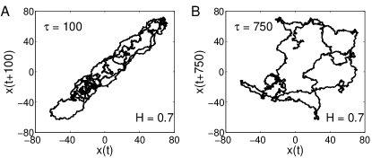
Figure 2: Example trajectory of a fBm with $H=0.7$ in a two-dimensional reconstructed phase space with embedding delays (A) $\tau=100$ and (B) $\tau=750$ ($N=2^{13}$).

To further illustrate the practical consequences of the observed behavior of the sample ACF when using embedding techniques, Fig. 2 displays the same realization of a fBm embedded in a two-dimensional space with different embedding delays $\tau$. Notably, the two embedding components are highly correlated for small $\tau$ but less correlated for larger $\tau$, leading to an entirely different geometric shape of the data object in the reconstructed phase space. The same behavior will be necessarily observed in higher embedding dimensions. As a consequence, a “practical” choice of the embedding delay for fBm should be independent of $H$, but depend on $N$. The numerical results presented above suggest $\tau\approx 2000$ for $N=2^{13}$ and $\tau\approx 8000$ for $N=2^{15}$, possibly generalizing to $\tau\approx N/4$. This is a rather large value, clearly far larger than those used by Liu et al. Liu et al. (2014) ($\tau\sim 10\dots 20$ for $N=2^{12}$).

The determination of a reasonable embedding dimension $m$ is often achieved by the FNN method Kennel et al. (1992). The criterion for the embedding dimension being high enough is that the fraction of false nearest-neighbors is zero or at least sufficiently small. Figure 3A displays our corresponding numerical results for fBm for three different lengths, which consistently suggest $m=4$.

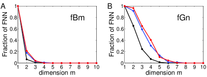
Figure 3: Fraction of false nearest-neighbors (FNN) for (A) fBm and (B) fGn with $H=0.7$ and different time series lengths $N$ (black: $N=1000$, blue: $N=21000$, and red: $N=31000$).

II.3 Choice of the recurrence threshold

An appropriate choice of the recurrence threshold $\varepsilon$ has attracted great interest in the literature on RNs Donner et al. (2010b, 2011a); Donges et al. (2012); Donner et al. (2015); Eroglu et al. (2014). The most wide-spread procedure is fixing the resulting recurrence rate $\rho$ (i.e., the fraction of recurrences) and adjusting $\varepsilon$ accordingly. As a rule-of-thumb, $\rho$ is often taken between about 0.01 and 0.05 for typical RN sizes of a few thousand vertices Marwan et al. (2007); Donner et al. (2010b), presenting a trade-off between the necessity of avoiding a largely disconnected network (too small $\epsilon$) and the interest in the geometric fine structure of the system in its phase space, which is hidden when considering too large spatial domains. The latter requirement has been more precisely formulated in Donges et al. (2012), emphasizing on the empirically expected relationship for the RN’s average path length, $\mathcal{L}(\varepsilon)\sim\varepsilon^{-1}$, which has been numerically confirmed Donner et al. (2010a); Donges et al. (2012).

Recently, Liu et al. (2014); Eroglu et al. (2014) suggested using the percolation threshold of the random geometric graph constructed from the given distribution of observed state vectors in phase space as a suitable lower bound to $\varepsilon$. As shown by Donges et al. (2012), the scaling of the RN’s average path length breaks down if $\varepsilon$ falls below the limit for which the RN decomposed into disjoint components, which is a necessary consequence of the fact that the averaging involved in the calculation of $\mathcal{L}$ is commonly considered only over pairs of vertices that are mutually reachable Donner et al. (2010a); Donges et al. (2012). However, when disregarding shortest path-based RN characteristics, there is no reason why one should restrict oneself to connected-networks, since other graph properties are hardly affected by the presence of more than one component. In particular, requesting the existence of a single component can lead to rather large $\varepsilon$ due to the presence of outliers in the data Donner et al. (2010b), especially in case of stochastic processes.

In this spirit, we recommend fixing $\rho$ at some reasonable value instead of tuning $\varepsilon$ according to the percolation threshold. Notably, in this case results obtained for different data sets still correspond to different $\varepsilon$ when they originate from independent realizations of stochastic processes. However, the problem of the dependence of some network measures on the number of edges in the RN is relieved in this case. Note that for fBm, due to the non-stationarity in variance the spread of state vectors in any reconstructed phase space necessarily grows with the sample size $N$.

III RN analysis of fGn processes

Based on our discussion presented in the previous section, we conclude that the results recently presented in Liu et al. (2014) hold only for the particular choices of the algorithmic parameters (for instance, length of time series, embeddings etc), showing limited physical interpretations. Moreover, using non-stationary time series data necessarily produces unreliable and spurious results.

One solution to the problem could be transforming the process in a way so that it becomes stationary. In recent applications to non-stationary real-world time series Donges et al. (2011b, a), the authors have removed non-stationarities in the mean by removing averages taken within sliding windows from the data. In the particular case of fBm, where non-stationary affects the variance, the underlying stochastic process can be transformed into a stationary one by a first-order difference filter, i.e., by considering its increments $x_{i+1}-x_{i}$. The transformed series is commonly referred to as fractional Gaussian noise (fGn) in analogy with the classical Brownian motion arising from an aggregation of Gaussian innovations. Notably, fGn retains the long-range correlations and Gaussian probability density function (PDF) from the underlying fBm process. For illustration purposes, three independent realizations of fGn with the same characteristic Hurst parameter $H=0.7$ are shown in Fig. 4A. Visual inspection clearly suggests the absence of non-stationarity in both mean and variance.

III.1 Embedding of fGn processes

Because of its stationarity, for fGn the estimated ACF shows a much faster decay and less ensemble spread than for fBm (Fig. 4B). Therefore, disregarding the conceptual limitations of this approach when considering stochastic processes, embedding parameters can be chosen more properly for fGn than for fBm. Concerning embedding delay $\tau$, one easily sees that $\tau=1$ is a natural choice for $H<0.5$ according to the classical ACF criterion, since the corresponding process is anti-persistent. Specifically, in this case the ACF drops to negative value at lag one (as shown in Fig. 4C), i.e., subsequent values are negatively correlated – the defining property of anti-persistence. In contrast, for $H>0.5$ we use the de-correlation time $\tau_{0.1}$ as an estimator for embedding delay $\tau$, which increases with rising $H$ as one would expect since larger $H$ indicates a longer temporal range of correlations.

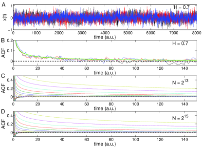
Figure 4: As in Fig. 1 for fGn obtained by differencing the previous fBms. In (B), the additional green line represents the averaged ACF over 200 independent realizations.

As before, the embedding dimension $m$ is chosen via the FNN method. In Fig. 3B, we show the fraction of false nearest-neighbors as $m$ is varied. Unlike for fBm, our results suggest that the optimal value $m$ rises with an increasing length of the time series. In general, considerably higher values of $m$ are suggested than for fBm, which matches the theoretical expectations more closely. However, due to the finite sample size, we still find a vanishing FNN rate at a finite embedding dimension, which is probably related to a lack of proper neighbors when high dimensions are considered.

III.2 Expected RN properties of stationary Gaussian processes

Given a proper representation of the considered system by its phase space reconstruction, the RN properties can be computed analytically from estimates of the underlying $m$-dimensional state density $p(\mathbf{x})$ Donges et al. (2012). In this spirit, an appropriate representation requires that the sample size is sufficient to cover all relevant parts of phase space, and that the sampling interval is reasonably chosen (i.e., to avoid sampling times co-prime with natural frequencies of continuous-time systems). For fBm, the latter condition cannot be fulfilled due to the non-stationarity of the process, whereas it is technically met for fGn processes.

Making use of the analytical results of Donges et al. (2012), we expect that the degree distribution $p(k)$ of the obtained RNs should be the same for any stationary process with Gaussian PDF given the same embedding dimension $m$. Specifically, this distribution has a complex shape Zou et al. (2012b) that is independent of $H$ (note that we may fix the mean degree $\left<k\right>$ by selecting a given $\rho=\left<k\right>/(N-1)$). In fact, this invariance is a direct consequence of the fact that the geometry of the data in phase space is not affected by $H$ when considering sufficiently de-correlated components, a requirement that has not been met by Liu et al. (2014) in their recent investigation of fBm as discussed above.

We emphasize again that the above considerations require a stationary Gaussian process and an embedding for which all components are as close as possible to being linearly independent. Otherwise, dependences between the components of the embedding vector lead to a deformation of the data distribution in phase space and, hence, possibly different geometric properties such as a too small effective dimension (i.e., smaller than $m$).

III.3 Transitivity properties

In Donner et al. (2011b), we have recently demonstrated that the RN characteristics transitivity $\mathcal{T}$ and global clustering coefficient $\mathcal{C}$ provide relevant information for characterizing the geometry of the resulted RNs, which has been numerically supported for various deterministic-chaotic systems. However, given the theory presented in Donges et al. (2012), the corresponding considerations can be extended to any kind of process or, more generally, any kind of random geometric graph Dall and Christensen (2002) with a given state density $p(\mathbf{x})$. Here, we exemplify these considerations for the case of fGn and examine how the transitivity properties of RNs arising from such stationary long-range correlated stochastic processes depend on the characteristic Hurst exponent as well as the underlying algorithmic parameters.

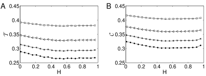
Figure 5: Dependence of (A) RN transitivity $\mathcal{T}$ and (B) global clustering coefficient $\mathcal{C}$ for fGn on the Hurst exponent $H$ for different embedding dimensions ($m=3$: $\square$, $m=4$: $\triangleleft$, $m=5$: $\ast$, $m=6$: $\bullet$), taken over 200 independent realizations and using a RN edge density of $\rho=0.03$. The embedding delay has been kept at the same value for all realizations with the same $H$ according to the de-correlation time $\tau_{0.1}$. In all cases, $N=2^{12}$.

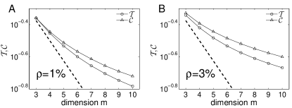
Figure 6: Dependence of RN transitivity $\mathcal{T}$ and global clustering coefficient $\mathcal{C}$ on the embedding dimension $m$ for fGn with $H=0.7$ (averages over 200 realizations) for two different values of $\rho$ ((A): $\rho=0.01$, (B): $\rho=0.03$). The dashed line corresponds to the expected analytical values $\mathcal{T}=(3/4)^{m}$ for $m$-dimensional Gaussian processes. In all cases, $N=2^{12}$.

For $H>0.5$, Fig. 5 shows that for a given embedding dimension $m$, both transitivity and global clustering coefficient do not depend on $H$. Following our above considerations, this is expected since the $m$-dimensional Gaussian PDF of the process does not depend on $H$, and the components are sufficiently de-correlated so that any marked geometric deformation of the embedded data is avoided. Hence, we construct RNs from the same PDF in all cases. Some minor deviation from the constant values can be observed at $H$ close to 1, i.e., close to the non-stationary limit case represented by $1/f$-noise, which might be due to numerical effects since the corresponding processes are harder to simulate than such with moderate $H$.

For $H<0.5$, the behavior changes markedly: both $\mathcal{T}$ and $\mathcal{C}$ rise with decreasing Hurst exponent. The reason for this behavior is that $\tau=1$ is the recommended, but still not “optimal” embedding delay for anti-persistent processes. Specifically, the closer $H$ approaches 0, the stronger is the anti-correlation at lag one. This means that with the same embedding delay $\tau=1$, the smaller $H$ the stronger are the mutual correlations between the different components of the embedding vector. As a consequence, the state vectors do not form a homogeneous $m$-dimensional Gaussian PDF with independent components in the reconstructed phase space, but are stretched and squeezed along certain directions, so that the resulting geometric structure appears significantly lower-dimensional than $m$.

Given that $\mathcal{T}$ ($\mathcal{C}$) is related to a geometric notion of the global (average local) dimension of the data Donner et al. (2011b), a reduced dimensionality of the data object results in a positive bias of both properties, which is exactly what we observe here (Fig. 5). Following the latter considerations, it is also easy to explain why both $\mathcal{T}$ and $\mathcal{C}$ systematically decrease with increasing embedding dimension $m$ (Figs. 5, 6). Specifically, for a random geometric graph in $m$ dimensions (computed with the maximum norm as also used in this work), one can show analytically that $\mathcal{T}=(3/4)^{m}$ Donner et al. (2011b) (similar considerations apply to $\mathcal{C}$ Donges et al. (2012)). For a fixed sample size $N$, however, this theoretical expectation is only met at low embedding dimensions $m$, whereas we find a systematic upward bias of both $\mathcal{T}$ and $\mathcal{C}$ as $m$ increases (Fig. 6). We explain the latter observation by the finite sample size together with the problem that proximity relationships become more ambiguous in higher dimensions when fixing a certain value of $\rho$. Therefore, it can be expected that the bias should be systematically reduced when using larger sample sizes $N$ together with smaller edge densities $\rho$ (for the latter effect, cf. Fig. 6A,B).

It would be straightforward to extend this kind of analysis to other network measures, since the available analytical description of RNs allows for their calculation as well Donges et al. (2012). We leave a corresponding discussion as a subject of future work.

IV Conclusions

By a critical reassessment of previous work Liu et al. (2014), we have identified several sources of errors when applying recurrence network analysis (or, in a similar way, other concepts based on recurrences in phase space) to long-range correlated stochastic processes. In summary, the main conclusions of this analysis are as follows:

1. RN analysis is based on phase space concepts originated in the theory of deterministic dynamical systems. Therefore, its potential application to stochastic processes requires special care.

2. The RN theory Donges et al. (2012); Donner et al. (2015) holds only for stationary processes. A direct application of RN analysis to typical non-stationary processes (in particular fBm) therefore has to fail, since the PDF of the process in the considered phase space changes with time. Without correcting for non-stationarity by a proper transformation of the series, the obtained results are commonly spurious.

3. A major problem associated with non-stationary processes is that embedding cannot be properly defined. In particular, the necessary selection of an embedding delay is ambiguous since auto-correlation function and related measures of serial dependences are not well-defined anymore.

4. For stationary stochastic processes, an embedding delay can be formally estimated from the data. However, the problem of selecting an embedding dimension remains, since stochastic processes are (in the viewpoint of dynamical systems theory) infinite-dimensional. Hence, any low-dimensional embedding of a stochastic process necessarily loses relevant information, which is a major cause of spurious results.

Despite the aforementioned conceptual problems and pitfalls resulting thereof, RN can still be used for obtaining interesting information on stationary stochastic processes. Drawing upon the interpretation of RNs as random geometric graphs Dall and Christensen (2002) in some reconstructed phase space, the network properties could in principle be computed solely from the multi-dimensional PDF of the embedded process. Deviations from the expectations are related to statistical dependencies between the different embedding components as well as finite-sample and finite-scale effects. The latter are also relevant for deterministic-chaotic processes, where in turn the underlying PDF can often not be calculated or at least estimated with high accuracy. In this spirit, deriving information based on stochastic processes can indeed help by providing benchmarks for studies of deterministic dynamics.

In general, applying RN analysis to scalar measurements requires an appropriate choice of embedding parameters. We do not claim that all choices made in this work have been based on fully objective quantitative criteria. The concepts like de-correlation time and false nearest-neighbors applied in this work rather present heuristics capturing only some aspects relevant for obtaining a proper phase space reconstruction. In this spirit, the results reported in Liu et al. (2014) are conceptually interesting but practically difficult to interpret. For systematic applications, the choice of embedding parameters depends on the particular process under consideration and should involve careful statistical evaluation beyond visual inspection.

Finally, we emphasize that for non-stationary systems, embedding parameters cannot be properly defined in general, so that any RN analysis (as well as other time series analysis techniques) necessarily yields systematic errors. This particularly applies to fBm and related processes arising from an integration of stationary processes (e.g., fractional Lévy motion, (F)ARIMA models, etc.). In such cases, a proper transformation is required to remove the particular type of non-stationarity from the data. This can be achieved by additive detrending, phase adjustment (de-seasonalization), difference filtering (incrementation) or other techniques, with the one mentioned last being the proper tool for the particular case of fBm transforming the original process into stationary fGn. Applying RN analysis to the latter indeed provides meaningful results. It should be noted that this observation is consistent with some wide-spread conceptual ideas beyond successful methodological alternatives for non-stationary time series analysis such as DFA Peng et al. (1994), which commonly make use of detrending and/or time series differentiation/aggregation. A more systematic exploration of corresponding approaches in combination with recurrence-based techniques is general, and RN analysis in particular, could be an interesting subject of future work.

Acknowledgements.

YZ acknowledges financial support by the NNSF of China (Grant Nos. 11305062, 11135001), the Specialized Research Fund (SRF) for the Doctoral Program (20130076120003), the SRF for ROCS, SEM, the Open Project Program of State Key Laboratory of Theoretical Physics, Institute of Theoretical Physics, Chinese Academy of Sciences, China (No.Y4KF151CJ1), and the German Academic Exchange Service (DAAD). RVD has been funded by the Federal Ministry for Education and Research (BMBF) via the Young Investigator’s group CoSy-CC² (project no. 01LN1306A).

References

- Kantz and Schreiber (2004) H. Kantz and T. Schreiber, Nonlinear time series analysis (Cambridge University Press, 2004), 2nd ed.
- Sprott (2003) J. C. Sprott, Chaos and Time-Series Analysis (Oxford University Press, Oxford, 2003).
- Poincaré (1890) H. Poincaré, Acta Mathematica 13, A3 (1890).
- Ott (2002) E. Ott, Chaos in Dynamical Systems (Cambridge University Press, Cambridge, 2002), 2nd ed.
- Xu et al. (2008) X. Xu, J. Zhang, and M. Small, Proc. Natl. Acad. Sci. USA 105, 19601 (2008).
- Marwan et al. (2009) N. Marwan, J. F. Donges, Y. Zou, R. V. Donner, and J. Kurths, Phys. Lett. A 373, 4246 (2009).
- Donner et al. (2010a) R. V. Donner, Y. Zou, J. F. Donges, N. Marwan, and J. Kurths, New J. Phys. 12, 033025 (2010a).
- Marwan et al. (2007) N. Marwan, M. C. Romano, M. Thiel, and J. Kurths, Phys. Rep. 438, 237 (2007).
- Eckmann et al. (1987) J.-P. Eckmann, S. O. Kamphorst, and D. Ruelle, Europhys. Lett. 4, 973 (1987).
- Mandelbrot and Van Ness (1968) B. Mandelbrot and J. Van Ness, SIAM Review 10, 422 (1968).
- Peng et al. (1994) C.-K. Peng, S. V. Buldyrev, S. Havlin, M. Simons, H. E. Stanley, and A. L. Goldberger, Phys. Rev. E 49, 1685 (1994).
- Kantelhardt et al. (2001) J. W. Kantelhardt, E. Koscielny-Bunde, H. H. Rego, S. Havlin, and A. Bunde, Physica A 295, 441 (2001).
- Hu et al. (2001) K. Hu, P. C. Ivanov, Z. Chen, P. Carpena, and H. Eugene Stanley, Phys. Rev. E 64, 011114 (2001).
- Bunde and Havlin (2002) A. Bunde and S. Havlin, Physica A 314, 15 (2002).
- Kantelhardt et al. (2003) J. W. Kantelhardt, T. Penzel, S. Rostig, H. F. Becker, S. Havlin, and A. Bunde, Physica A 319, 447 (2003).
- Liu et al. (2014) J.-L. Liu, Z.-G. Yu, and V. Anh, Phys. Rev. E 89, 032814 (2014).
- Donges et al. (2011a) J. F. Donges, R. V. Donner, M. H. Trauth, N. Marwan, H. J. Schellnhuber, and J. Kurths, Proc. Natl. Acad. Sci. USA 108, 20422 (2011a).
- Donges et al. (2011b) J. F. Donges, R. V. Donner, K. Rehfeld, N. Marwan, M. H. Trauth, and J. Kurths, Nonlin. Proc. Geophys. 18, 545 (2011b).
- Donner et al. (2010b) R. V. Donner, Y. Zou, J. F. Donges, N. Marwan, and J. Kurths, Phys. Rev. E 81, 015101(R) (2010b).
- Strozzi et al. (2011) F. Strozzi, K. Poljansek, F. Bono, E. Gutiérrez, and J. Zaldıvar, International Journal of Bifurcation and Chaos 21, 1047 (2011).
- Donges et al. (2012) J. F. Donges, J. Heitzig, R. V. Donner, and J. Kurths, Phys. Rev. E 85, 046105 (2012).
- Donner et al. (2011a) R. V. Donner, M. Small, J. F. Donges, N. Marwan, Y. Zou, R. Xiang, and J. Kurths, Int. J. Bifurcation Chaos 21, 1019 (2011a).
- Zou et al. (2010) Y. Zou, R. V. Donner, J. F. Donges, N. Marwan, and J. Kurths, Chaos 20, 043130 (2010).
- Zou et al. (2012a) Y. Zou, R. V. Donner, and J. Kurths, Chaos 22, 013115 (2012a).
- Grebogi et al. (1984) C. Grebogi, E. Ott, S. Pelikan, and J. A. Yorke, Physica D: Nonlinear Phenomena 13, 261 (1984).
- Feudel et al. (2006) U. Feudel, S. Kuznetsov, and A. Pikovsky, Strange Nonchaotic Attractors – Dynamics between Order and Chaos in Quasiperiodically Forced Systems (World Scientific, Singapore, 2006).
- Donner et al. (2011b) R. V. Donner, J. Heitzig, J. F. Donges, Y. Zou, N. Marwan, and J. Kurths, Eur. Phys. J. B 84, 653 (2011b).
- Takens (1981) F. Takens, in Dynamical Systems and Turbulence, Warwick 1980, edited by D. A. Rand and L.-S. Young (Springer, New York, 1981), vol. 898 of Lecture Notes in Mathematics, pp. 366–381.
- Kennel et al. (1992) M. B. Kennel, R. Brown, and H. D. I. Abarbanel, Phys. Rev. A 45, 3403 (1992).
- Fraser and Swinney (1986) A. M. Fraser and H. L. Swinney, Phys. Rev. A 33, 1134 (1986).
- Grassberger and Procaccia (1983) P. Grassberger and I. Procaccia, Physica D 9, 189 (1983).
- Mandelbrot (1982) B. Mandelbrot, The Fractal Geometry of Nature (W. H. Freeman, New York, 1982).
- Gneiting and Schlather (2004) T. Gneiting and M. Schlather, SIAM Review 46, 269 (2004).
- Witt and Malamud (2013) A. Witt and B. Malamud, Surveys in Geophysics 34, 541 (2013), ISSN 0169-3298.
- Donner et al. (2015) R. V. Donner, J. F. Donges, Y. Zou, and J. H. Feldhoff, in Recurrence Quantification Analysis, edited by C. L. Webber, Jr. and N. Marwan (Springer International Publishing, 2015), Understanding Complex Systems, pp. 101–163, ISBN 978-3-319-07154-1.
- Eroglu et al. (2014) D. Eroglu, N. Marwan, S. Prasad, and J. Kurths, Nonlinear Processes in Geophysics Discussions 1, 803 (2014).
- Zou et al. (2012b) Y. Zou, J. Heitzig, R. V. Donner, J. F. Donges, J. D. Farmer, R. Meucci, S. Euzzor, N. Marwan, and J. Kurths, Europhys. Lett. 98, 48001 (2012b).
- Dall and Christensen (2002) J. Dall and M. Christensen, Phys. Rev. E 66, 016121 (2002).