Abstract

We focus in this paper on the effect of the resolution of Direct Numerical Simulations (DNS) on the spatio-temporal development of the turbulence downstream of a single square grid. The aims of this study are to validate our numerical approach by comparing experimental and numerical one-point statistics downstream of a single square grid and then investigate how the resolution is impacting the dynamics of the flow. In particular, using the $Q$-$R$ diagram, we focus on the interaction between the strain-rate and rotation tensors, the symmetric and skew-symmetric parts of the velocity gradient tensor respectively. We first show good agreement between our simulations and hot-wire experiment for one-point statistics on the centreline of the single square grid. Then, by analysing the shape of the $Q$-$R$ diagram for various streamwise locations, we evaluate the ability of under-resolved DNS to capture the main features of the turbulence downstream of the single square grid.

1 Introduction

The most accurate approach to simulate a turbulent flow is to solve the Navier-Stokes equations without averaging, extra modelling assumptions and parameterisations (e.g. sub-grid) or approximations other than numerical discretisations. This approach is called Direct Numerical Simulation (DNS) and is the simplest approach conceptually because all the motions of the flow are supposed to be resolved. Because of the enormous range of scales in time and in space which need to be resolved, DNS of turbulent flows can become very expensive in terms of computational resources and is therefore often only used for the understanding of the fundamental features of turbulence in relatively simple flow configurations such as periodic homogeneous isotropic turbulence or turbulent channel flows [19].

With recent impressive developments in computer technology, it is now possible to undertake DNS with a very large number of mesh nodes to study turbulent flows at relatively high Reynolds numbers in more complex configurations than homogeneous isotropic turbulence. One of the main difficulties however is to determine the spatial resolution of a DNS, as this choice is related to the range of scales that need to be accurately represented. The resolution requirements are obviously influenced by the numerical method used and the usefulness of highly accurate numerical schemes for DNS is fully recognized, the most spectacular gain being obtained with spectral methods based on Fourier or Chebyshev representation [2].

The number of mesh points required to capture the smallest scales in a DNS is most of the time estimated following Kolmogorov’s phenomenology [10, 11]. Assuming that all the scales smaller than the Kolmogorov scale $\eta$ are dissipated and cannot contribute to the inertial range dynamics, it is usually established that the number of mesh points $N$ required in a DNS of homogeneous isotropic turbulence of dimension $L_{b}^{3}$ can be estimated with the relation $N\approx(L_{b}/\eta)^{3}\sim Re_{L_{b}}^{9/4}$ where $Re_{L_{b}}$ is the Reynolds number based on $L_{b}$ (which is representative of the integral scale $L$) and the rms of the fluctuating velocity $u^{\prime}$. This relation was first shown in 1959 by [16] and is nowadays widely used in many studies based on DNS. It is important to point out that this relation is assuming local isotropy for the flow and an average dissipation approximated with $\langle\varepsilon\rangle\approx C_{\varepsilon}u^{\prime 3}/L_{b}$, with $C_{\varepsilon}$ defined as a constant [30, 9]. It is also possible to estimate the cost in terms of time steps $T/\Delta t$ with $T\approx L_{b}/u^{\prime}$ corresponding to the timescale related to the dimension $L_{b}$ of the cubic box. Assuming that $u^{\prime}\Delta t\approx\Delta x$, we obtain $T/\Delta t\sim Re_{L_{b}}^{3/4}$ if $\Delta x\sim\eta$ [9]. These estimates can be used to evaluate the computational power $W$ required to perform a DNS. If we have $\eta\approx\Delta x$ then $W$ scales as $(L_{b}/\Delta x)^{3}(T/\Delta t)\approx Re_{L_{b}}^{3}$. This means that doubling the Reynolds number requires nearly an order of magnitude increase in computational effort.

In recent years several authors have been debating these relations and whether they are accurate enough to evaluate high-order derivatives and high order statistics. In [4], the authors investigated resolution effects and scaling in DNS of homogeneous isotropic turbulence with a special attention to dissipation and enstrophy, with resolutions of up to $\Delta x/\eta=0.25$. They confirmed that the formula to evaluate the resolution of a DNS of statistically steady forced periodic turbulence designed to resolve the smallest scales of the flow within a constant multiple $a$ of $\eta$ and with a computational box whose linear size $L_{b}$ is a constant multiple $b$ of the largest scale of the flow, i.e. the integral scale $L$, can be approximated as $N\approx 0.05\frac{b}{a}Re^{4.5}_{\lambda}$. This formula is very similar to the previous formula, assuming that $Re_{\lambda}\sim Re_{L}^{0.5}$. They showed that, in the context of statistically stationary homogeneous isotropic forced turbulence, this standard resolution is adequate for computing second-order quantities but is underestimating high-order moments of velocity gradients. They demonstrated that the smallest scale that needs to be resolved to capture high-order quantities (of order $n$, with $n\rightarrow\infty$) is $\eta_{min}\approx LRe^{-2}_{\lambda}$. In [31], the authors state that the computational power needed to perform a DNS of fully developed homogeneous isotropic turbulence increases as $Re_{L}^{4}$ if ones want to study high-order quantities, and not as the $Re_{L}^{3}$ expected from Kolmogorov’s theory.

In practice, the previous estimates can be a little tricky to use and recent work suggests that they do not apply to a wide enough range of turbulent flows. Indeed, it has recently been shown that $C_{\epsilon}$ is not constant in a substantial region of spatially evolving fully developed turbulent flows such as decaying grid-generated turbulence and axisymmetric turbulent wakes [30, 14, 21] and is also not constant in unsteady periodic turbulence [8]. In all these cases $C_{\epsilon}$ is proportional to the ratio of a global inlet/initial Reynolds number $Re_{I}$ to a local (in time or space) Reynolds number $Re_{L}$ based on $u^{\prime}$ and an integral length-scale $L$. This has of course direct implications on DNS resolution requirements as $C_{\epsilon}$ is taken to be constant in the aforementioned resolution estimates. In the case of a DNS of unsteady periodic turbulence, such as the one of [8] for example, this new scaling of $C_{\epsilon}$ implies that $N\sim(L/\eta)^{3}\sim C_{\epsilon}^{3/4}Re_{L}^{9/4}\sim Re_{I}^{3/4}Re_{L}^{3/2}$. In the case of more realistic turbulent flows, and therefore more complicated, than periodic turbulence, such as the turbulent flows considered in this paper, the resolution estimates based on periodic homogeneous isotropic turbulence are neither directly nor easily applicable.

Even though it is now possible to reach relatively high Reynolds numbers using DNS, only very limited comparisons with experimental data have been documented in order to evaluate the quality of a DNS. Comparisons between hot-wire anemometry and DNS were carried out for a fully turbulent pipe flow at a Reynolds number $Re_{c}\approx 7000$ based on centreline velocity and pipe diameter [5]. The resolution of their DNS followed the rule $\Delta\leq\pi\eta$ with the use of a uniform cylindrical mesh in the three spatial direction.The agreement between numerical and experimental results was excellent for the lower-order statistics (mean flow and turbulence intensities) and reasonably good for the higher-order statistics (skewness and flatness factors of the normal-to-the-wall velocity fluctuations).

[20] performed single point hot-wire measurements in a turbulent channel flow at $Re_{\tau}=934$ and compared their data with the DNS of [1] at the same friction velocity Reynolds number $Re_{\tau}$. Results showed excellent agreement between the streamwise velocity statistics of the two data sets. The spectra were also very similar, however, throughout the logarithmic region the secondary peak in energy was clearly reduced in the DNS results because of the DNS box length, leading to the recommendation that longer box lengths should be investigated.

In [25] the authors performed the first direct comparisons between DNS and wind tunnel hot-wire and oil-film inerferometry measurements of a turbulent zero-pressure-gradient boundary layer at Reynolds numbers up to $Re_{\theta}=2500$. They found excellent agreement in skin friction, mean velocity and turbulent fluctuations. However, they did point out that such comparisons can be made difficult by, for instance, the choice tripping which can affect the onset of transition to turbulence.

Note, finally, that the resolution in all these DNS as well as in other recent DNS of high Reynolds number periodic turbulence [32], turbulent boundary layers [26, 6] and turbulent mixing layers [1] are all following the rule $\eta<\Delta x<3\eta$.

Our goal in the present numerical work is to assess the quality and resolution requirements of DNS of a spatially developing turbulent flow generated by a single square grid [33] against hot-wire measurements in a wind tunnel. We investigate how the resolution affects the fluid motion and special attention is given to the effects of the quality and reliability of the numerical data on small-scale statistics. For this, we focus on the strain-rate and rotation tensors (the symmetric and skew-symmetric parts of the velocity gradient tensor respectively) through a detailed analysis of Q-R diagrams [27] at various locations downstream of the single square grid on the centreline of the flow.

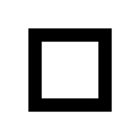
Figure 1: Sketch of the single square grid used in the simulations (left) and in the experiments (right).

2 Numerical set-up

The single square grid represented in figure 1 (left) is defined using $L_{0}$ as the lateral length of each bar and $t_{0}$ as their lateral thickness, with $L_{0}=5.30t_{0}$. The streamwise thickness of the grid is $0.25t_{0}$. The computational domain $L_{x}\times L_{y}\times L_{z}=8L_{0}\times 2L_{0}\times 2L_{0}$ is discretized on a Cartesian mesh using $n_{x}\times n_{y}\times n_{z}=2881\times 720\times 720$ mesh nodes for the highly resolved $SSG$-$HR$ (Single Square Grid - High Resolution) simulation, $n_{x}\times n_{y}\times n_{z}=1441\times 360\times 360$ mesh nodes for the low resolution $SSG$-$LR$ (Single Square Grid - Low Resolution) simulation and $n_{x}\times n_{y}\times n_{z}=721\times 180\times 180$ mesh nodes for the ultra low resolution $SSG$-$ULR$ (Single Square Grid - Ultra Low Resolution) simulation. The coordinates $x$, $y$, and $z$ correspond to the streamwise and the two cross-flow directions respectively. The origin is placed at the centre of the single square grid, which is located at a distance of $1.25L_{0}$ from the inlet of the computational domain in order to avoid spurious interactions between the grid and the inlet condition. The blockage ratio $\sigma$ for this single square grid is $19\%$. Inflow/outflow boundary conditions are used in the streamwise direction while periodic boundary conditions are used in the two lateral directions. The inflow condition is a uniform profile $U_{\infty}$ free from any perturbations whereas the outflow condition is a standard 1D convection equation. For this numerical work, after the evacuation of the initial condition, data are collected over a period of $500,000$ time steps (with a time step of $0.000139L_{0}/U_{\infty}$). In terms of Reynolds number based on $L_{0}$, $Re_{L_{O}}=21,600$ for the three simulations.

Figure 2: Evolution of the spatial resolution with respect to the Kolmogorov microscale $\Delta x/\eta$ (left), and of the normalised dissipation $\varepsilon L_{0}/U^{3}_{\infty}$ (right) along the centreline where $x_{*}=L_{0}^{2}/t_{0}$, is the wake interaction length-scale [7]. For the single square grid case, the turbulence along the centreline reaches a maximum value at $x_{peak}\approx 0.5x_{*}$.

In order to quantify the resolution with respect to the smallest scales of the flow, we plot in figure 2 (left) the streamwise evolution of $\Delta x/\eta$ along the centreline $y=z=0$, where $\eta$ is the Kolmogorov microscale defined as $(\nu^{3}/\epsilon_{full})^{1/4}$. The dissipation $\varepsilon_{full}$ is evaluated using $\varepsilon_{full}=2\nu\langle(\partial u^{\prime}_{i}/\partial x_{j})^{2}\rangle$. The full dissipation and the dissipation $\varepsilon_{iso}=15\nu\langle(\partial u_{1}^{\prime}/\partial x_{1})^{2}\rangle$, which is obtained assuming the isotropy of the flow, are plotted in figure 2 (right). It can be seen that the full dissipation and the isotropic dissipation are virtually the same except maybe for the simulation with the lowest resolution for which marginal differences can be spotted. As expected, when the mesh is not fine enough to capture the smallest scales of the flow, as for the $SSG$-$ULR$ simulation, the dissipation at the smallest scales cannot be taken into account and is therefore underestimated by approximatively a factor two. The $SSG$-$LR$ and $SSG$-$HR$ simulations are producing similar levels for the dissipation. For the simulation with the finest mesh, $\Delta x/\eta$ is always smaller than 2, whereas for the coarsest mesh, $\Delta x/\eta$ is always smaller than 7. As a reference, in their recent very high Reynolds number Direct Numerical simulations of wall bounded turbulence, the authors in [6] have a comparable resolution with $\Delta x/\eta<2$. We are therefore expecting the mesh from the $SSG$-$HR$ simulation to be fine enough to take into account the smallest features of the flow and a good comparison with experiments can be expected.

3 Numerical method

The incompressible Navier-Stokes equations are solved using a recent version of the high-order flow solver Incompact3d, adapted to parallel supercomputers using a powerful 2D domain decomposition strategy [13]. This code is based on sixth-order compact finite difference schemes for the spatial differentiation and an explicit third order Adams-Bashforth scheme for the time integration. To treat the incompressibility condition, a fractional step method requires solving a Poisson equation. This equation is fully solved in spectral space, via the use of relevant 3D Fast Fourier Transforms. The pressure mesh is staggered from the velocity mesh by half a mesh, to avoid spurious pressure oscillations. With the help of the concept of modified wave number, the divergence-free condition is ensured up to machine accuracy. The modelling of the grid is performed using an Immersed Boundary Method (IBM) based on direct forcing approach that ensures the no-slip boundary condition at the obstacle walls. The idea is to force the velocity to zero at the wall of the single square grid, as our particular Cartesian mesh does conform with the geometries of the grid. It mimics the effects of a solid surface on the fluid with an extra forcing in the Navier-Stokes equations. Full details about the code can be found in [12].

4 Experimental set-up

In order to provide data for comparison with the simulations, experiments were conducted with a very similar grid, as shown in figure 1 (right), in a blow down wind tunnel, whose working section has a square cross-section of 0.4572m $\times$ 0.4572m (18” $\times$ 18”) and a working length of 3.5m, with the turbulence generating grids placed at the start of the test-section. The background turbulence level is 0.1%. A grid is installed at the entrance of the diffuser to maintain a slight over-pressure in the test section. The inlet velocity $U_{\infty}$ is controlled using the static pressure difference across the 8:1 contraction, the temperature taken near the diffuser and the atmospheric pressure from a pressure gauge, all of which were measured using a Furness Controls micromanometer FCO510.

Measurements of the velocity signal on the centreline of the flow were taken using a DANTEC 55P01 hot-wire ($5\mu m$ in diameter with a sensing length of 1.25mm), driven by a DANTEC Streamline anemometer with an in-build signal conditioner running in constant-temperature mode (CTA). Data was sampled using a 16-bit National Instruments NI-6229(USB) data acquisition card for $300sec$ at a sampling frequency of 100kHz, with the analogue low-pass filter on the Streamline set to 30kHz. Each data set was then digitally filtered, using a fourth-order Butterworth filter to eliminate high frequency noise, at a frequency of $f_{c}\geq 1.5f_{\eta}$, where $f_{\eta}=\langle u\rangle/2\pi\eta$, where $\langle u\rangle$ is the local mean streamwise velocity. The blockage ratio for the grid in the experiments is slightly larger than the one in the simulations with a value of $21\%$, because of the addition of the small bars to hold the single square grid in the wind tunnel. In terms of Reynolds numbers based on $L_{0}=228.6mm$, $Re_{L_{O}}=36450$, $72,900$ and $145,900$, corresponding to an inflow velocity $U_{\infty}$ of $2.5m/s$, $5m/s$ and $10m/s$.

Note that the Reynolds number $Re_{L_{0}}$ in the three simulations is about 1.7 times smaller than the smallest Reynolds number of the experiments as it was not possible to reduce the speed of the wind tunnel below $2.5m/s$. Because of computational constraints for the simulation with the highest resolution, the collection time $T=16sec$ for the simulations, corresponding to $500,000$ time-steps, is much smaller than in the experiments where it is $T=300sec$. One substantial difference between the experimental and numerical set-ups is in the boundary conditions, walls in the wind tunnel as opposed to periodic boundary conditions in the simulations. However, because of the low blockage ratio of the single square grid, we do not expect a significant impact of the walls and/or the boundary conditions on the centreline of the grid where we evaluate the quality of the simulations.

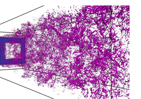
Figure 3: Turbulent flows generated by the single square grid for the $SSG$-$HR$ simulation; 3D isosurfaces equal to 0.5 of the absolute value of the enstrophy vector normalised by its maximum over the ($y-z$) plane at the $x$-position considered.

5 Comparison with experiments

An illustration of the flow obtained downstream of the single square grid is given in figure 3, where enstrophy isosurfaces are plotted. These isosurfaces are showing the enstrophy normalised by its maximum over the ($y-z$) plane at the $x$-position considered. The four same-size wakes generated by the four bars of the grid interact and mix together to give rise to a fully turbulent flow.

We first compare, along the centreline of the flow, the streamwise evolutions of the local mean streamwise velocity $\langle u\rangle$ and of the streamwise turbulence intensity $\sqrt{\langle u\rangle^{\prime 2}}$. The results, presented in figure 4, are normalised with $x_{*}=L_{0}^{2}/t_{0}$ which is the wake interaction length-scale [7]. For the single square grid case, the turbulence along the centreline reaches a maximum value at $x_{peak}\approx 0.5x_{*}$ both for experimental and numerical data. For the experimental data, it can be seen that there is a maximum value of about 1.6 for $\langle u\rangle/U_{\infty}$ located at $x=0.1x_{*}$, followed by a fast decay up to $x=0.3x_{*}$, and then a slow decay up to $x=x_{*}$. After that point, the effect of the boundary layers at the wall of the wind tunnel can eventually be seen for the experimental data with a very slow increase of $\langle u\rangle/U_{\infty}$. The $SSG$-$HR$ and $SSG$-$LR$ simulations are in very good agreement with the experiments both quantitatively and qualitatively, with for instance the correct prediction of the maximum value 1.62 at $x=0.1x_{*}$. The data for the $SSG$-$HR$ simulation and the experiments are even on top of each other up to $x=x_{*}$. The $SSG$-$ULR$ simulation is under predicting the streamwise evolution of $\langle u\rangle/U_{\infty}$. For instance, the maximum value for $\langle u\rangle$ is under estimated by about $10\%$ with a value of only 1.467 at $x=0.075x_{*}$. Concerning the evolution of $\sqrt{\langle u\rangle^{\prime 2}}$, only the $SSG$-$HR$ simulation is able to predict correctly the location of the peak and its intensity. An important result here is the over estimation by SSG-ULR of $\sqrt{\langle u\rangle^{\prime 2}}$ in the production region before the peak of turbulence. This could be attributed to a pile-up of energy due to the lack of dissipation in the simulation, with the creation of numerical spurious oscillations just downstream of the single square grid where the resolution for the smallest scales is not good enough. After the peak, the three simulations are in relative good agreement with the experimental data, even in those cases where the location of the peak of turbulence was not predicted properly.

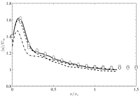
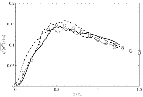
Figure 4: Evolution of the local mean streamwise velocity $\langle u\rangle$ normalised with $U_{\infty}$ (left) and of the streamwise turbulence intensity $\sqrt{\langle u\rangle^{\prime 2}}$ normalised with the local mean streamwise velocity $\langle u\rangle$ (right) along the centreline. The continuous line corresponds to $SSG$-$HR$, the dashed line to $SSG$-$LR$ and the dot-dashed line to $SSG$-$ULR$. The symbols correspond to the experiments with $\Diamond$$=10m/s$, $\Box$$=5m/s$, $\circ$$=2.5m/s$.

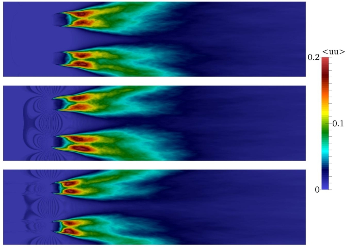
Figure 5: Contour map of $<u^{\prime 2}>/U_{\infty}^{2}$ in the $xy$ plane at z=0. From top to bottom: $SSG$-$HR$, $SSG$-$LR$ and $SSG$-$ULR$.

The effect of the resolution can clearly be seen in figure 5 where a 2D map of $\langle u^{\prime 2}\rangle/U^{2}_{\infty}$ is plotted in the $(x-y)$ plane for $z=0$. In front of the grid, spurious oscillations appear when the resolution is not good enough. It is the signature of the pile-up of energy at the small scales. As already observed on the centreline, these oscillations seem to have to have a relatively low impact on the dynamic of the flow downstream of the grid.

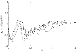
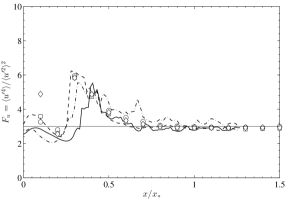
Figure 6: Evolution of the skewness (left) and the flatness (right) of the fluctuating streamwise velocity. The continuous line corresponds to $SSG$-$HR$, the dashed line to $SSG$-$LR$ and the dot-dashed line to $SSG$-$ULR$. The symbols correspond to the experiments with $\Diamond$$=10m/s$, $\Box$$=5m/s$, $\circ$$=2.5m/s$.

Figure 6 shows the streamwise evolution of the skewness $S_{u}$ and of the flatness $F_{u}$ of the streamwise turbulence intensity where

$$S_{u}=\frac{\langle u^{\prime 3}\rangle}{\langle u^{\prime 2}\rangle^{3/2}},~{}~{}~{}~{}~{}~{}~{}~{}~{}F_{u}=\frac{\langle u^{\prime 4}\rangle}{\langle u^{\prime 2}\rangle^{2}}$$ (1)

It is clear that the numerical data are not converged enough to get a smooth profile for the streamwise evolution. However, the numerical data are in good quantitative agreement with the experiments as they are following the same trend. In the production region, the values obtained for the skewness and the flatness suggest that the distribution of the velocity is highly non-Gaussian both for the experiments and for the simulations. This is related to the presence of strong events in the flow, as reported previously by [18, 33], in the production region of grid-generated turbulence. After the peak of turbulence located at $x=0.5x_{*}$, the skewness is converging to zero and the flatness is converging to 3, corresponding to a Gaussian distribution for the streamwise turbulence intensity.

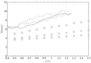
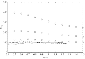
Figure 7: Evolution of the Taylor micro-scale $\lambda$ (left) and of the associated local Reynolds number (right). The continuous line corresponds to $SSG$-$HR$, the dashed line to $SSG$-$LR$ and the dot-dashed line to $SSG$-$ULR$. The symbols correspond to the experiments with $\Diamond$$=10m/s$, $\Box$$=5m/s$, $\circ$$=2.5m/s$.

Figure 7 shows the streamwise evolution of the Taylor micro-scale $\lambda$ and of the associated local Reynolds number, where

$$\lambda\approx\sqrt{\frac{\langle u^{\prime 2}\rangle}{\left\langle\left(\frac{1}{\langle u\rangle}\frac{\partial u^{\prime}}{\partial t}\right)^{2}\right\rangle}}$$

As expected, $\lambda$ is slowly increasing after the peak of turbulence (located at $\approx 0.5x_{*}$) when moving downstream of the grid. When the inflow velocity is increased, $\lambda$ is reduced. The values obtained between $4mm$ and $10mm$ are consistent with previous values obtained experimentally for a fractal square grid by [28] where values between $4mm$ and $6mm$ were reported for an inflow velocity of $15m/s$. A notable result is that for the DNS data and for the experimental data with the lowest velocity, $Re_{\lambda}$ remains constant after the peak of turbulence (located at $\approx 0.5x_{*}$). It is a rather surprising result which could be attributed to the low inflow velocity of the flow but which is in good agreement with the numerical results of [33]. In [29] it was shown experimentally that for a very similar grid, $Re_{\lambda}$ was decreasing after the peak of turbulence, which is consistent with the current experimental data. The present results are therefore suggesting that the new dissipation law [30], for which $C_{\epsilon}$ is not constant, is valid above a certain value for $Re_{\lambda}$, value which is grid-dependant.

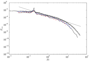
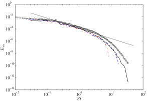
Figure 8: Energy spectra of the streamwise fluctuating velocity component at $0.4x_{*}$ (left) and at $x_{*}$ (right). The continuous line corresponds to $SSG$-$HR$, the dashed line to $SSG$-$LR$ and the dot-dashed line to $SSG$-$ULR$. The symbols correspond to the experiments with $U_{\infty}=2.5m/s$.

In order to investigate a bit further the quality of the simulations, the energy spectra obtained at $0.4x_{*}$ and at $x_{*}$ for the streamwise turbulence intensity $\sqrt{u^{\prime 2}}$ are presented in figure 8. These energy spectra, obtained in the frequency domain on the centreline of the flow are estimated using the periodogram technique [23]. Data are collected in time for the simulations using virtual probes in a similar fashion to the experiments. The time signal is then divided in several sequences with an overlap of $50\%$ with the use of a Hanning window. The cut-off frequency for the simulations is $f_{c}=U_{\infty}/2\Delta x$, corresponding to the smallest frequency that the mesh can see and for the experiments we have $f_{c}=1.5f_{\eta}$, where $f_{\eta}=\langle u\rangle/2\pi\eta$. The energy spectra plots obtained at $0.4x_{*}$ in the production region are showing a very good agreement between the experiments and the simulations with the correct prediction of the Strouhal, corresponding to the frequencies of the large scale vortices generated by the single square grid. As expected, the levels of energy are slightly larger in the experiment, as the inflow velocity and therefore the global Reynolds number are higher. Interestingly enough, the energy spectra for the three simulations in the production region are following the same trend and it is difficult to observe any resolution effect near the cut-off frequency of each simulations. However, in the decay region after the peak of turbulence, there is a clear drop-off of the energy spectra near the cut-off frequency for the three simulations, as seen in figure 8 for $x=x_{*}$. Note also that the cut-off frequency of the experiments is the same as the one for the high-resolution simulation, suggesting that this simulation is able to capture the smallest scales of the flow. From a physical point of view, both the experiments and the simulations exhibit -5/3 frequency spectra for at least one decade of frequencies.

6 Effect of the resolution on the turbulence

Following our previous work with fractal square grids [15] and the recent work of [33] with a single square grid, it is possible to obtain some information about the resolution effects on vorticity and strain rate statistics using the $Q$-$R$ diagram [27].

The velocity gradient tensor $A_{ij}=\partial u_{i}/\partial x_{j}$ can be decomposed in a symmetric part $S_{ij}=(\partial u_{i}/\partial x_{j}+\partial u_{j}/\partial x_{i})/2$ and an anti-symmetric part $W_{ij}=(\partial u_{i}/\partial x_{j}-\partial u_{j}/\partial x_{i})/2$. $S_{ij}$ is defined as the strain rate tensor and $W_{ij}$ as the rotation rate tensor. Eigenvalues of $A_{ij}$ satisfy the following characteristic equation

$$\lambda^{3}+P\lambda^{2}+R\lambda+R=0,$$ (2)

with

$$P=-A_{ii},$$ (3)

$$Q=-\frac{1}{2}A_{ij}A_{ji},$$ (4)

$$R=-\frac{1}{3}A_{ij}A_{jk}A_{ki}.$$ (5)

When the flow is incompressible, then $P=0$. Furthermore, one can decompose $Q$ and $R$ as

$$Q=\frac{1}{4}(\omega_{i}\omega_{i}-2S_{ij}S_{ij})=Q_{w}+Q_{s},$$ (6)

with $Q_{w}=\frac{1}{4}\omega_{i}\omega_{i}$, $Q_{s}=-\frac{1}{2}S_{ij}S_{ij}$ and

$$R=-\frac{1}{3}(S_{ij}S_{jk}S_{ki}+\frac{3}{4}\omega_{i}\omega_{j}S_{ij})=R_{w}+R_{s},$$ (7)

with $R_{s}=-\frac{1}{3}S_{ij}S_{jk}S_{ki}$, $R_{w}=-\frac{1}{4}\omega_{i}\omega_{j}S_{ij}$ and $\omega_{i}=\varepsilon_{ijk}\partial u_{j}/\partial x_{k}$, $\varepsilon_{ijk}$ being the Levi-Civita symbol.

The $Q$-$R$ diagram has a tear drop shape in many turbulent flows (turbulent boundary layers, mixing layers, grid turbulence, jet turbulence) and according to [27], this tear drop shape may be one of the qualitatively universal features of turbulent flows. Therefore, it is a good indicator to assess the quality of our simulations and check how the lack of resolution can affect the $Q$-$R$ diagram.

Figure 9: Joint probability density function of $Q$ and $R$ for periodic, statistically stationary turbulence from a DNS courtesy of Dr. R. Onishi, see [22] for details. The dark red colour corresponds to isovalues greater than 0.025. Note that these statistics were obtained over all space at single snapshot in time.

As a reference, we are using the numerical data of a DNS of periodic statistically stationary turbulence [22]. The $Q$-$R$ diagram obtained from a single time shot is presented in figure 9. Note that $Q$ is normalised with $\langle S_{ij}S_{ij}\rangle$ and $R$ by $\langle S_{ij}S_{ij}\rangle^{3/2}$. As expected we can observed the tear drop shape when $Q<0$ and $R>0$.

Figure 10: Streamwise evolution of $\langle Q_{w}\rangle$, $\langle Q_{s}\rangle$, $\langle R_{w}\rangle$ and $\langle R_{s}\rangle$ along the centreline for the single square grid.

In Figure 10 we plot the streamwise evolution of $\langle Q_{w}\rangle$, $\langle Q_{s}\rangle$ as functions of $x/x_{*}$ as well as $\langle R_{w}\rangle$, $\langle R_{s}\rangle$ along the centreline for the three simulations. Note that $\langle.\rangle$ means an average in time for a particular point in space. The first important result is that $\langle Q\rangle=\langle Q_{w}\rangle+\langle Q_{s}\rangle$ and $\langle R\rangle=\langle R_{w}\rangle+\langle R_{s}\rangle$ along the centreline of the flow are very close to zero for the three simulations, as expected in homogeneous isotropic turbulence. This is not a trivial result as already stated by [15] because grid-generated turbulence is not homogeneous just downstream of the grid in the production region where the four wakes are mixing together. The plots in Figure 10 for the $SSG$-$HR$ and $SSG$-$LR$ simulations are very similar, the only difference being the small shift for the peak of the plotted quantities that is slightly earlier in the case of the $SSG$-$LR$ simulation. For the simulation $SSG$-$ULR$ both the location and the intensity of the peak are impacted by the poor resolution. As already observed by [15] for a fractal square grid, $<Q_{w}>$ and $<R_{w}>$ are very close to zero between $x/x_{*}=0$ and $x/x_{*}=0.3$. This can be observed for the three simulations. The location of the first non-zero values of average enstrophy and enstrophy production rates is however different for the three simulations. This can be related to the pile-up of energy at the small scales due to the low resolution, resulting in spurious numerical enstrophy where the flow should be irrotational.

In order to better investigate the behaviour of the flow in the region $0<x/x_{*}<0.3$, we plot in figure 11 the streamwise evolution of $\langle-Q_{w}/Q_{s}\rangle$ and of $\langle-R_{w}/R_{s}\rangle$ on the centreline of the flow. The effect of the resolution can clearly be seen very close to the grid where the ratios $\langle-Q_{w}/Q_{s}\rangle$ and $\langle-R_{w}/R_{s}\rangle$ are virtually zero for the simulation with the highest resolution whereas they are clearly non-zero for the two other simulations. Based on the $SSG$-$HR$ simulation, we can say that $Q_{s}$ and $R_{s}$ are much larger than $Q_{w}$ and $R_{w}$ respectively, meaning that $Q_{w}$ should be virtually zero in the region $0<x/x_{*}<0.3$ along the centreline. It is a confirmation that the pile-up of energy for the simulations at low resolutions is creating numerical spurious enstrophy which can be seen in $Q_{w}$ and $R_{w}$. After $0.3x_{*}$, the three simulations are giving the same result with $\langle-Q_{w}/Q_{s}\rangle\approx\langle-R_{w}/R_{s}\rangle\approx 1$.

Figure 11: Streamwise evolution of $\langle-Q_{w}/Q_{s}\rangle$ and $\langle-R_{w}/R_{s}\rangle$ along the centreline for the three simulations

It is of interest to see how the $Q$-$R$ diagram is evolving downstream of the single square grid and how it is affected by the resolution of the simulations. The plots presented in figure 12, 13, 14 and 15 are obtained for four streamwise locations corresponding to $x=0.08x_{*},~{}0.2x_{*},0.5x_{*}$ and $x_{*}$ and are based on data collected in time over a period equivalent to $T=16sec$. As suspected, there is a clear difference very close to the grid between the three simulations as shown in figure 12 at $x=0.08x_{*}$. Based on the simulation with the best resolution, the flow should be dominated by flow regions where $R<0$ and $Q<0$, as already observed by [33] in a very similar flow configuration. The trend is less obvious with the intermediate resolution whereas the simulation with the lowest resolution is producing a completely different $Q$-$R$ diagram with a tear drop shape for $Q<0$ and $R>0$.

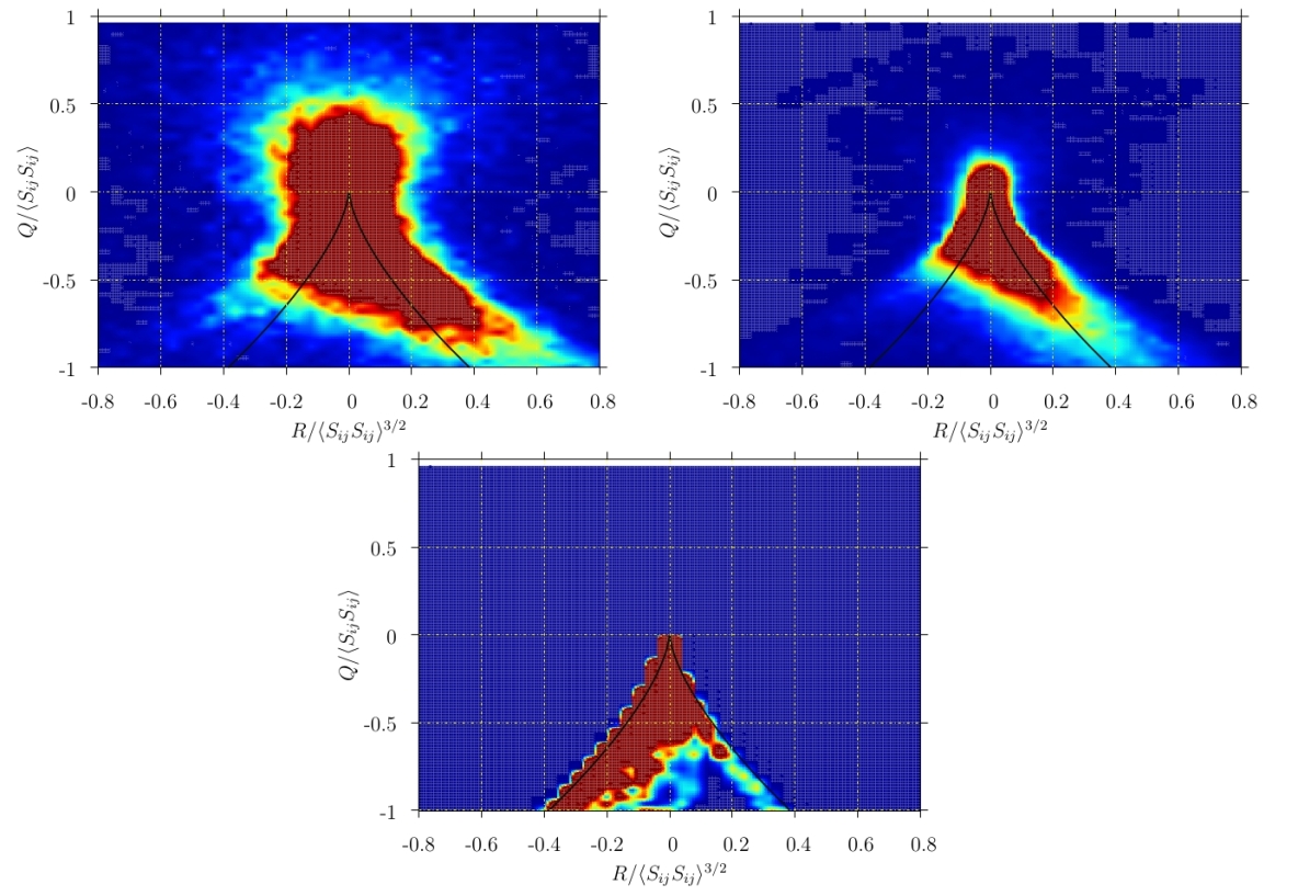
Figure 12: Joint probability density function for the $Q$-$R$ diagram obtained at $x=0.08x_{*}$ for the $SSG$-$ULR$ (top left), $SSG$-$LR$ (top right) and $SSG$-$HR$ (bottom) simulations.

Further downstream, at $x=0.2x_{*}$, the $Q$-$R$ diagram is quite different with a flow dominated by flow regions where $R>0$ and $Q<0$ as shown in figure 13. It should be noted that $Q$ is almost always negative at this point which shows that there is still no enstrophy at this streamwise location. The $Q$-$R$ diagram obtained here is very similar to the ones obtained by [3] in the non rotational region surrounding a spatially evolving turbulent jet. The $SSG$-$HR$ and $SSG$-$LR$ simulations are in fairly good agreement with each other for this location. The simulation with the lowest resolution is producing a nearly symmetric $Q$-$R$ diagram, meaning that it is not possible to track any fluid flow dynamics at this resolution using the $Q$-$R$ diagram. It is consistent with the pile-up of energy at the small scales, altering the flow motion at this location. We will see later that this nearly symmetric shape for the $Q$-$R$ diagram is also the signature of a random white noise field [27].

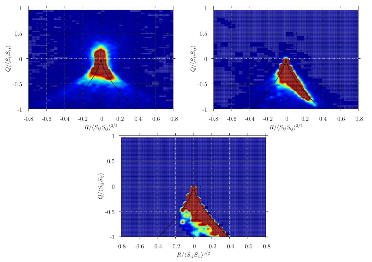
Figure 13: Joint probability density function for the $Q$-$R$ diagram obtained at $x=0.2x_{*}$ for the $SSG$-$ULR$ (top left), $SSG$-$LR$ (top right) and $SSG$-$HR$ (bottom) simulations.

For $x=0.5x_{*}$, we can see in figure 14 that the $Q$-$R$ diagram is at the beginning of adopting its usual tear drop shape. At this location, the effect of the resolution is less pronounced, the only difference being the size of the dark red region which is slightly larger when the resolution is decreased. Note that this streamwise location is in the decay region for the turbulence, just after the peak shown in figure 4.

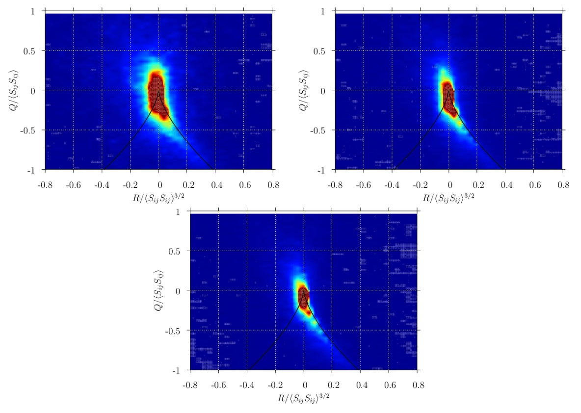
Figure 14: Joint probability density function for the $Q$-$R$ diagram obtained at $x=0.5x_{*}$ for the $SSG$-$ULR$ (top left), $SSG$-$LR$ (top right) and $SSG$-$HR$ (bottom) simulations.

Finally, further downstream in the decay region for $x=x_{*}$, it can be seen in figure 15 that the $Q$-$R$ diagram has a tear drop shape and that the resolution is not damaging this tear drop shape. This suggests that in this region, the pile-up of energy at the small scales is not affecting the flow motion, at least not enough to strongly impact the $Q$-$R$ diagram.

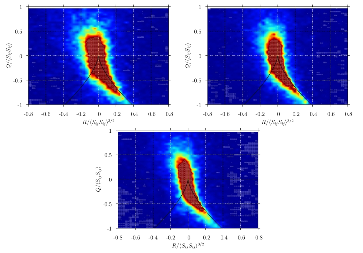
Figure 15: Joint probability density function for the $Q$-$R$ diagram obtained at $x=x_{*}$ for the $SSG$-$ULR$ (top left), $SSG$-$LR$ (top right) and $SSG$-$HR$ (bottom) simulations.

In order to better understand the effect of the small-scale pile-up of energy on the $Q$-$R$ diagram, we are now going to filter the data where the pile-up of energy is damaging the $Q$-$R$ diagram and see if it is possible to recover the diagram obtained with the simulation with the highest resolution. The filtering procedure is based on the sixth-order compact operator proposed by [17]

$$\frac{3}{10}\hat{f}_{i-2}+\hat{f}_{i}+\frac{3}{10}\hat{f}_{i+2}=\frac{1}{2}f_{i}+\frac{3}{8}(f_{i+1}-f_{i-1})+\frac{3}{20}(f_{i+2}-f_{i-2})+\frac{1}{40}(f_{i+3}-f_{i-3})$$ (8)

with $f_{i}=f(x_{i})$, $\hat{f}_{i}=\hat{f}(x_{i})$ and $x_{i}=(i-1)\Delta x$ for $(i=1,...,n_{x})$, all those quantities being defined for $[0,L_{x}]$. $\hat{f}(x_{i})$ corresponds to the filtered quantity. The associated filtering transfer function $T(k)$ is

$$T(k)=\frac{1/2+(3/4)\cos(k)+(3/10)\cos(k)+(1/20)\cos(k)}{1+(3/5)\cos(2k)}$$ (9)

and is plotted in Figure 16. The filter operator, applied in the three spatial directions on the three components of the velocity, can be see as a low pass filter for which the filtering effect is confined to the shortest wavelengths. In the present work, the filter operator is applied 250 times to each 3D snapshot of the $SSG$-$LR$ simulation, corresponding to the elimination of the smallest scales of the flow up to $10\eta$. It is necessary to apply the filter operator 250 times in order to have clean 3D snapshots free of any numerical oscillations. As shown in Figure 16, it corresponds to a filter width of about $3.5\Delta x$. Then the $Q$-$R$ diagram is produced from the filtered data and is compared with the $Q$-$R$ diagram obtained from the $SSG$-$HR$ simulation at the same location. Note that the $Q$-$R$ diagrams are not computed in time any more. Each $Q$-$R$ diagram presented in figures 15 to 19 is obtained from a single snapshot in a small 3D cube $0.025x_{*}\times 0.025x_{*}\times 0.025x_{*}$ around a specific streamwise location on the centreline. We have checked over our different uncorrelated snaphots that the data presented in this study are representative of the flow dynamics for a given streamwise location.

Figure 16: Filtering transfer function $T(k)$ versus wave number $k$ for the sixth-order compact operator (8) used in this work.

First, to validate our filtering procedure, we take a snapshot from the $SSG$-$HR$ simulation, superimpose a random white noise to it to mimic the numerical oscillations due to the pile-up of energy at the small scales and then filter the altered snapshot with the aim to recover the $Q$-$R$ diagram produced by the clean snapshot. In figure 17, three $Q$-$R$ diagrams are presented. They are obtained for the $SSG$-$HR$ simulation at $x=0.2x_{*}$. The first important result is that the $Q$-$R$ diagram shown in figure 17 (top left) is very similar to the one obtained at the same location with the data in time (see figure 13 bottom). The $Q$-$R$ diagram presented in figure 17 (top right) is obtained with a random white noise superimposed to the velocity field. This noise corresponds to a $0.025\%$ uncertainty in the mean value of $U_{\infty}$. The shape of the $Q$-$R$ diagram is perfectly symmetric and is very similar to the one obtained for the $SSG-ULR$ simulation at $x=0.2x_{*}$ (see figure 13 top left). It means that the pile-up of energy at the small scales and the random noise are damaging the $Q$-$R$ diagram in a similar fashion. Furthermore, for this particular location, the $Q$-$R$ diagram is clearly dominated by the added random noise (or by the low resolution). When the filtering procedure is applied to the data with a superimposed random white noise, the $Q$-$R$ diagram observed in figure 17 (bottom) is very similar to the one obtained for the raw data.

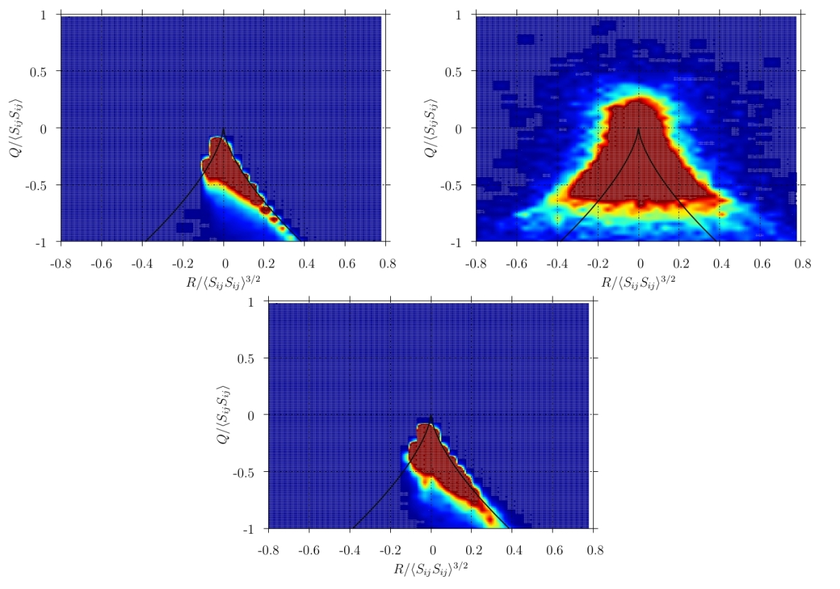
Figure 17: Joint probability density function for the $Q$-$R$ diagrams obtained from the $SSG$-$HR$ simulation at $x=0.2x_{*}$ for a ($0.025x_{*}\times 0.025x_{*}\times 0.025x_{*}$) cube (125,000 mesh nodes) with no added random noise and no filtering (top left), with added random noise (top right) and with added random noise and filtering (bottom).

The same procedure is repeated downstream of the grid at $x=0.6x_{*}$. The data are presented in figure 18. It can be seen that the addition of a random white noise has only a limited impact on the $Q$-$R$ diagram, the only visible difference being a reduced tear drop tail and a broadening of the dark red region, as already observed by [24] in a turbulent mixing layer flow. As expected, the effect of the filtering procedure on the data with a superimposed random white noise is also quite limited, suggesting that for this particular location, the $Q$-$R$ diagram is mainly dominated by large scale structure features. The alteration of the small scales at this streamwise location seems to be quite limited on strain-rate and rotation tensors. It is worth pointing out that there is a big difference between adding spurious noise to a well-resolved set of data and having spurious numerical artefacts in an under-resolved DNS in which the dynamics among all the scales maybe incorrectly reproduced. For this numerical investigation, we are just trying to find a way to filter under-resolved DNS data to better understand how the resolution is affecting the strain-rate and rotation tensors.

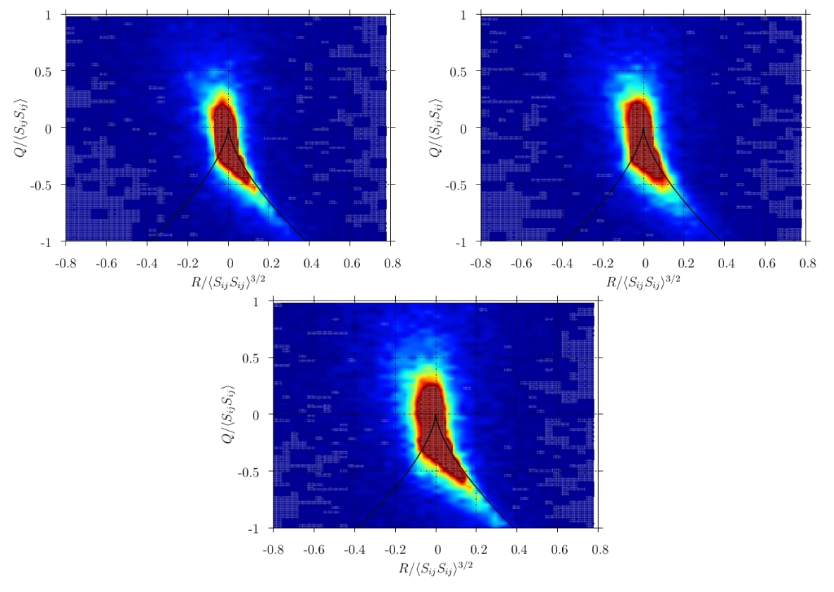
Figure 18: Joint probability density function for the $Q$-$R$ diagrams obtained from the $SSG$-$HR$ simulation at $x=0.6x_{*}$ for a ($0.025x_{*}\times 0.025x_{*}\times 0.025x_{*}$) cube (125,000 mesh nodes) with no added random noise and no filtering (top left), with added random noise (top right) and with added random noise and filtering (bottom).

The filtering procedure is now applied to a set of snapshots obtained from the $SSG$-$LR$ simulation where spurious numerical artefacts are present. Figure 19 shows the $Q$-$R$ diagram obtained before and after the filtering procedure for a ($0.025x_{*}\times 0.025x_{*}\times 0.025x_{*}$) cube (15,625 mesh nodes) located at $x=0.2x_{*}$ on the centreline. We can see that the non-filtered snapshots are producing a symmetric shape for the $Q$-$R$ diagram with positive values for $Q$, signature of spurious enstrophy caused by the pile-up of energy at the small scales. When the data are filtered, all the positive values of $Q$ are removed and the $Q$-$R$ diagram has a similar shape to the one obtained with the $SSG$-$HR$ simulation for the same location, with negative values of $Q$ weakly skewed toward $R>0$.

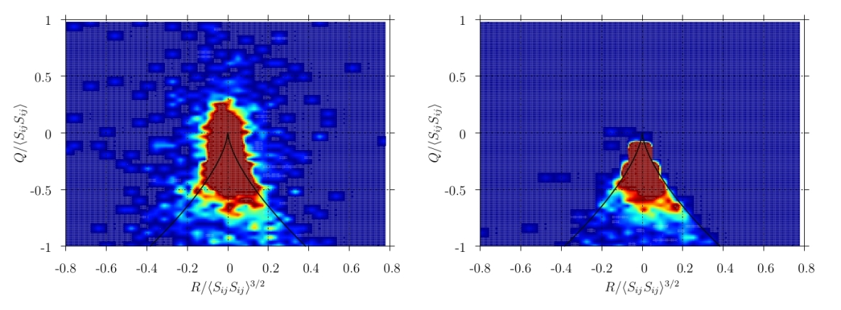
Figure 19: Joint probability density function for the $Q$-$R$ diagrams obtained from the $SSG$-$LR$ simulation at $x=0.2x_{*}$ for a ($0.025x_{*}\times 0.025x_{*}\times 0.025x_{*}$) cube (15,625 mesh nodes) with no filtering (left) and with filtering (right).

Further downstream for $x=0.6x_{*}$, the usual tear drop shape can be observed for both the non-filtered and filtered data, as shown in figure 20. Like previously observed for the $SSG$-$HR$ simulation for which random white noise was added, it seems that the spurious numerical errors for the small scales are not impacting too much the shape of the $Q$-$R$ diagram. The main difference between the filtered data and the non-filtered data is the size of the dark region which is larger when the data are filtered, with more data points for $Q>0$. It is a notable result, suggesting that an under-resolved DNS can qualitatively predict the behaviour of the strain-rate and rotation tensors at least when the flow is dominated by large scale features.

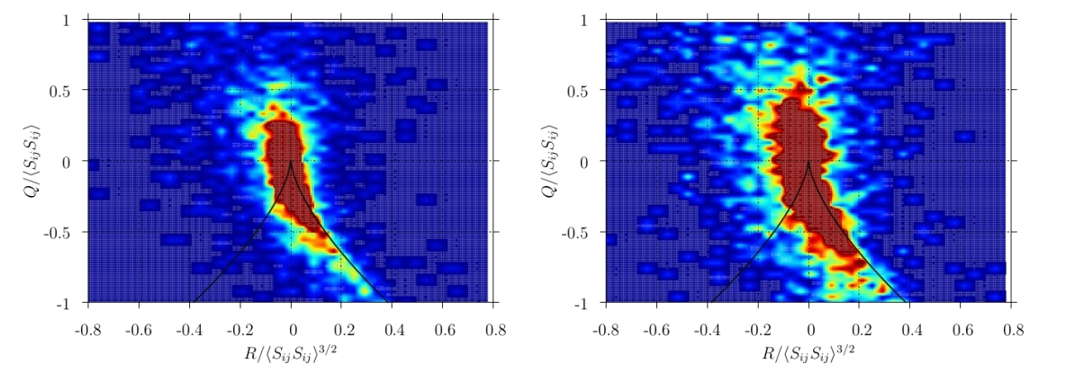
Figure 20: Joint probability density function for the $Q$-$R$ diagrams obtained from the $SSG$-$LR$ simulation at $x=0.6x_{*}$ for a ($0.025x_{*}\times 0.025x_{*}\times 0.025x_{*}$) cube (15,625 mesh nodes) with no filtering (left) and with filtering (right).

7 Conclusion

Direct Numerical Simulations of the turbulence generated by a single square grid have been presented in this paper in order to investigate the influence of the spatial resolution on fine-scale features and in particular on the strain-rate and rotation tensors. Careful comparisons with hot-wire experiments have been carried out on the centreline of the flow for first, second, third and fourth order moments of one-point flow velocities. For those quantities, we show that even the simulation with the lowest resolution ($\Delta x$ at worse equal to $7\eta$, at best equal to $2\eta$) is able to reproduce the experimental results within an error margin of about $10\%$. For the third and fourth order moments, it seems that the numerical data are not converged enough in time and the quality of the present numerical data would be greatly improved by increasing the level of convergence by one order of magnitude or two. For the first and second order moments, a resolution of $\Delta x\approx 5\eta$ seems to be enough to match experimental data within a margin of $5\%$.

Concerning the $Q-R$ diagram and the strain-rate and rotation tensors, the results are strongly dependent on both the resolution and the streamwise location. In the production region, upstream of the peak of turbulence, the flow is dominated by strain ($Q<0$ for the simulation $DNS-HR$) and the resolution is deeply impacting the small-scale features of the flow with positive values for $Q$ through the addition of spurious numerical artefacts when the spatial resolution is worse than $4\eta$, at least for our code Incompact3d, based on sixth-order finite-difference schemes on a Cartesian mesh. The $Q-R$ diagram can be used in our code as an indicator of the presence in the flow of non-physical features. The influence of our numerical artefacts on the $Q-R$ are similar to a random white noise. In the decay region, where the usual tear drop shape is observed for all the simulations, it is more difficult to quantify the influence of spurious numerical artefacts using the $Q-R$ diagram. The only noticeable difference is an increase of the size of the $Q-R$ diagram when the spatial resolution is decreased. The conclusion is that it is necessary to have a very fine spatial resolution of less than $2\eta$ for a correct reproduction of the strain-rate and rotation tensors.

References

- [1] A. Attili and F. Bisetti. Statistics and scaling of turbulence in a spatially developing mixing layer at re= 250. Phys. Fluids, 24(3):035109, 2012.
- [2] C. Canuto, M. Y. Hussaini, A. Quarteroni, and T. A. Zang. Spectral Methods in Fluid Dynamics. Springer-Verlag, New York, 1988.
- [3] C.B. da Silva and J.C.F. Pereira. Invariants of the velocity-gradient, rate-of-strain, and rate-of-rotation tensors across the turbulent/nonturbulent interface in jets. Physics of Fluids (1994-present), 20(5):055101, 2008.
- [4] D.A. Donzis, P.K. Yeung, and K.R. Sreenivasan. Dissipation and enstrophy in isotropic turbulence: Resolution effects and scaling in direct numerical simulations. Phys. Fluids, 20(4):045108, 2008.
- [5] J.G.M. Eggels, F. Unger, M.H. Weiss, J. Westerweel, R.J. Adrian, R. Friedrich, and F.T.M. Nieuwstadt. Fully developed turbulent pipe flow: a comparison between direct numerical simulation and experiment. J. Fluid Mech., 268:175–210, 1994.
- [6] G. Eitel-Amor, R. Örlü, and P. Schlatter. Simulation and validation of a spatially evolving turbulent boundary layer up to re= 8300. International Journal of Heat and Fluid Flow, 47:57–69, 2014.
- [7] R. Gomes-Fernandes, B. Ganapathisubramani, and J. C. Vassilicos. PIV study of fractal-generated turbulence. J. Fluid Mech., 701:306–336, 2012.
- [8] S. Goto and J.C. Vassilicos. Energy dissipation and flux laws for unsteady turbulence. Phys. Rev. Lett., submitted to, 2014.
- [9] T. Ishihara, T. Gotoh, and Y. Kaneda. Study of high-reynolds number isotropic turbulence by direct numerical simulation. Ann. Rev. Fluid Mech., 41:165–180, 2009.
- [10] A.N. Kolmogorov. Dissipation of energy in locally isotropic turbulence. Dolk. Akad. Nauk SSSR, 32:19–21, 1941.
- [11] A.N. Kolmogorov. The local structure of turbulence in incompressible viscous fluid for very large reynolds numbers. Dolk. Akad. Nauk SSSR, 30:299–303, 1941.
- [12] S. Laizet and E. Lamballais. High-order compact schemes for incompressible flows: a simple and efficient method with the quasi-spectral accuracy. J. Comp. Phys., 228(16):5989–6015, 2009.
- [13] S. Laizet and N. Li. Incompact3d, a powerful tool to tackle turbulence problems with up to computational cores. Int. J. Numer. Methods Fluids, 67(11):1735–1757, 2011.
- [14] S. Laizet and J.C. Vassilicos. Stirring and scalar transfer by grid-generated turbulence in the presence of a mean scalar gradient. J. Fluid Mech., in revision, 2014.
- [15] S. Laizet, J.C. Vassilicos, and C. Cambon. Interscale energy transfer in decaying turbulence and vorticity–strain-rate dynamics in grid-generated turbulence. Fluid Dynamics Research, 45(6):061408, 2013.
- [16] L.D. Landau and E.M. Lifshitz. Fluid mechanics, 1959. Course of Theoretical Physics, 1959.
- [17] S. K. Lele. Compact finite difference schemes with spectral-like resolution. J. Comp. Phys., 103:16–42, 1992.
- [18] N. Mazellier and J. C. Vassilicos. Turbulence without Richardson-Kolmogorov cascade. Phys. Fluids, 22(075101), 2010.
- [19] P. Moin and K. Mahesh. Direct numerical simulation: a tool in turbulence research. Ann. Rev. Fluid Mech., 30(1):539–578, 1998.
- [20] J.P. Monty and M.S. Chong. Turbulent channel flow: comparison of streamwise velocity data from experiments and direct numerical simulation. J. Fluid Mech., 633:461–474, 2009.
- [21] J. Nedić, J.C. Vassilicos, and B. Ganapathisubramani. Axisymmetric turbulent wakes with new nonequilibrium similarity scalings. Phys. Rev. Lett., 111(14):144503, 2013.
- [22] R. Onishi, Y. Baba, and K. Takahashi. Large-scale forcing with less communication in finite-difference simulations of stationary isotropic turbulence. J. Comp. Phys., 230:4088–4099, 2011.
- [23] W. H. Press, S.A. Teukolsky, W.T. Vetterling, and B.P. Flannery. Numerical Recipes. Cambridge University Press, Cambridge, 1992.
- [24] O.R.H. Buxton S., Laizet, and B. Ganapathisubramani. The effects of resolution and noise on kinematic features of fine-scale turbulence. Exp. Fluids, 51(5):1417–1437, 2011.
- [25] P. Schlatter, R. Orlu, Q. Qiang, G. Brethouwer, J.H.M. Fransson, A.V. Johansson, P.H. Alfredsson, and D.S. Henningson. Turbulent boundary layers up to studied through simulation and experiment. Phys. Fluids, 21(5):51702, 2009.
- [26] J.A. Sillero, J. Jiménez, and R.D. Moser. One-point statistics for turbulent wall-bounded flows at reynolds numbers up to . Phys. Fluids, 25:105102, 2013.
- [27] A. Tsinober. An informal conceptual introduction to turbulence. Springer, 2009.
- [28] P. Valente and J. C. Vassilicos. The decay of turbulence generated by a class of multi-scale grids. J. Fluid Mech., 687:300–340, 2011.
- [29] P. Valente and J. C. Vassilicos. Universal dissipation scaling for non-equilibrium turbulence. Phys. Rev. Lett., 108:214503, 2012.
- [30] J.C. Vassilicos. Dissipation in turbulent flows. Ann. Rev. Fluid Mech., available online:http://www.annualreviews.org/toc/fluid/forthcoming, 2015.
- [31] V. Yakhot and K.R. Sreenivasan. Anomalous scaling of structure functions and dynamic constraints on turbulence simulations. J. of statistical physics, 121(5-6):823–841, 2005.
- [32] P.K. Yeung, D.A. Donzis, and K.R. Sreenivasan. Dissipation, enstrophy and pressure statistics in turbulence simulations at high reynolds numbers. J. Fluid Mech., 700:5–15, 2012.
- [33] Y. Zhou, K. Nagata, Y. Sakai, H. Suzuki, Y. Ito, O. Terashima, and T. Hayase. Development of turbulence behind the single square grid. Phys. Fluids, 26(4):045102, 2014.