Tight asymptotic bounds on local hypothesis testing between a pure bipartite state and the white noise state

Abstract

We consider asymptotic hypothesis testing (or state discrimination with asymmetric treatment of errors) between an arbitrary fixed bipartite pure state $|\Psi\rangle$ and the white noise state (the completely mixed state) under one-way LOCC (local operations and classical communications), two-way LOCC, and separable POVMs. As a result, we derive the Hoeffding bounds under two-way LOCC POVMs and separable POVMs. Further, we derive a Stein’s lemma type of optimal error exponents under one-way LOCC, two-way LOCC, and separable POVMs up to the third order, which clarifies the difference between one-way and two-way LOCC POVM. Our results clarify the relationship between the entanglement of Renyi entropy and the hypothesis testing under LOCC, since the entanglement of Renyi entropy appears in the formula of both the Hoeffding bounds and the Stein’s lemma type of error exponents. Our study gives a very rare example in which the optimal performance under the infinite-round two-way LOCC is also equal to that under separable operations and can be attained with two-round communication, but not with the one-way LOCC.

I Introduction

When a quantum system consists of two distinct parties, Alice and Bob, it is natural to restrict their operations to local operation and classical communication (LOCC) [1] because it is not so easy to realize a quantum operation across both of the distant parties. LOCC operations can be classified by the direction of classical communication. When the direction of classical communication is restricted to only one direction, the LOCC operation is called a one-way LOCC. Otherwise, it is called a two-way LOCC. Such constraint for our measurement is called a locality restriction. In this paper, we focus on the effect for distinguishing quantum states. Such a state discrimination problem has been studied very actively by many researchers [2, 3, 4, 5, 6, 7, 8, 9, 10, 11, 12, 13, 14, 15, 16, 17, 18, 19, 20, 21, 22, 23, 24, 25, 26, 27, 28, 29, 30].

In this paper, we concentrate on the detection of a given entangled state from the completely mixed state, which is often called the white noise state because it has no biased noise. Since this problem deals with two states as candidates for the true state in an asymmetric way, it is usually referred to as the binary simple hypothesis testing. Since we impose the locality restriction, we call it the local hypothesis testing. Since, as was pointed out from a Shannon theoretical viewpoint [31, 32, 33, 34, 35, 36, 37, 39, 38, 40, 41, 42], hypothesis testing is related to so many information theoretic problems, quantum hypothesis testing with the asymptotic and asymmetric setting has attracted much attention in quantum information theory [30, 42, 45, 47, 48, 44, 43, 49, 53, 50, 51, 52, 46]. In order to discuss the relation between the locality constraint and these information theoretic problems, it is natural to deeply investigate quantum hypothesis testing with locality restriction.

One might consider that hypothesis testing with the white noise state is too specialized. However, as known in classical information theory, this type of hypothesis testing is directly related to data compression [32, 36], uniform random generation [32], channel coding with additive noise [31], and resolvability of distribution [41]. Thus, this problem can be regarded as the first step for extending these topics to the case with the locality constraint. Indeed, based on a similar motivation, a recent paper [50] treats the hypothesis testing of quantum channel with a special case as a quantum extension of a special case of the paper [54]. Further, hypothesis testing even with the white noise state is highly non-trivial when we impose any locality restriction, although it is trivial without one. Hence, this problem represents the difficulty caused by the locality restriction in the simplest way, and it can be considered as one of the most important types of local hypothesis testing. Therefore, to characterize the accessible information under locality condition, we tackle the local hypothesis testing with the white noise state in this paper.

On the other hand, since this problem can be described in terms of the entangled pure state to be detected, this problem is closely related to the amount of entanglement of the entangled pure state. Hence, it has a great significance as a study of entanglement. In fact, several entanglement measures have been proposed even for pure entangled states. One is the entanglement of entropy [55], and its relation with hypothesis testing with the white noise state has been clarified [56]. As other measures, the geometric measure of entanglement [57] and the robustness of entanglement [58] are known. However, their relations with this problem have only been partially resolved [56]. To discuss the relation between entanglement measures and hypothesis testing, we employ the entanglement of Rényi entropy [59], i.e., the Rényi entropy of the reduced density matrix of a pure entangled state, which contains the entanglement of entropy, the geometric measure of entanglement, and the logarithmic robustness of entanglement as special cases. Since Rényi entropy is also closely related to the asymptotic performance of quantum information protocols, we may predict that the entanglement of Renyi entropy is also closely related to the asymptotic performance of quantum information processing under the locality condition. In this paper, we show that this prediction is correct. That is, we clarify the relation between our hypothesis testing problem and the entanglement of Rényi entropy.

Before discussing the history of the local hypothesis testing, we focus on the quantum hypothesis testing without a locality condition, in which a general asymptotic theory can be established even for the quantum case where multiple copies of unknown states are available. Firstly, Hiai et al. [43] and Ogawa et al. [44] derived the quantum version of Stein’s bound [60], i.e., the optimal exponent of the type-2 error under the constant constraint for the type-1 error. Audenaert et al. [61] and Nussbaum et al. [62] derived the quantum version of the Chernoff bound [60], i.e., the optimal exponent of the sum of type-1 and type-2 errors. Other papers [37, 47] derived the quantum version of the Hoeffding bound [63, 65, 64], which is the optimal exponent of the type-2 error under the exponential constraint for the type-1 error and can be considered to be a generalization of the Chernoff bound. However, when we impose the one-way or two-way LOCC constraint on our measurement, these problems become very difficult, and they have not been solved completely. In particular, it is quite difficult to solve these problems for an arbitrary fixed pair of quantum states. In the following, we mainly address the Hoeffding bound and will hardly mention the Chernoff bound. This treatment does not lose generality because our results for the Hoeffding bound include the results for the Chernoff bound as special cases.

Before proceeding to the detailed discussion of the local hypothesis testing between a pure entangled state $|\Psi\rangle$ and the white noise state, we prepare a detailed classification of two-way LOCC operation. whereas a one-way LOCC operation requires only one-round classical communication, a two-way LOCC operation requires multiple-round classical communication. In this case, a two-way LOCC protocol with $k$-round classical communication has $k+1$ steps. For example, in the case of two-round classical communication, the total protocol is given as follows when the initial operation is done by Alice: Alice performs her operation with her measurement and sends her outcome to Bob. Bob receives Alice’s outcome, performs his operation with his measurement, and sends his outcome to Alice. Alice then receives Bob’s outcome and performs her measurement. Therefore, we focus on the difference among these locality restrictions. under the local hypothesis testing between a pure entangled state and the white noise state.

In the non-asymptotic setting, our previous paper [15] addressed the problem under the constraint that $|\Psi\rangle$ is detected with probability $1$. Our more recent paper [66] addressed it in a more general setting. In particular, that paper [66] proposed concrete two-round classical communication two-way LOCC protocols that are not reduced to one-way LOCC. Then, we extended the problem to the case when the entangled state is given as the $n$-copy state of a certain entangled state [56]. As asymptotic results, we showed that there is no difference between one-way and two-way LOCC for Stein’s bound, i.e., the optimal exponent of the type-2 error under the constant constraint for the type-1 error. To make an upper bound of the optimal performance of the two-way LOCC case, our papers [15, 56, 66] also considered the performance for separable operations, which can be easily treated because of their mathematically simple forms. The class of separable operations includes LOCC, but there exist separable operations that are not LOCC [3]. Unfortunately, our previous paper [56] could not derive the Hoeffding bound for two-way LOCC, i.e., the optimal exponent of the type-2 error under the exponential constraint for the type-1 error, while it derived it for one-way LOCC. Further, even under the constant constraint for the type-1 error, the paper did not consider the higher order of the decreasing rate of the type-2 error. Indeed, in information theory, Strassen [67] derived the decreasing rate of the type-2 error up to the third-order $\log n$ under the same constraint in the classical setting when $n$ is the number of available copies. Tomamichel et al. [42] and Li [48] extended this result up to the second-order $\sqrt{n}$.

In this paper, we derive the Hoeffding bound for two-way LOCC and the optimal decreasing rate of the type-2 error under the constant constraint for the type-1 error up to the third-order $\log n$ for one-way and two-way LOCC. We also derive them for separable measurements. The obtained results are summarized as follows.

(1)

There is a difference in the Hoeffding bound between the one-way and two-way LOCC constraints unless the entangled state $|\Psi\rangle$ is maximally entangled.

(2)

There is no difference in the Hoeffding bound between two-way LOCC and separable constraints.

(3)

The optimal decreasing rate of the type-2 error under the constant constraint for the type-1 error has no difference between the one-way and two-way LOCC constraints up to the second-order $\sqrt{n}$.

(4)

The optimal decreasing rate of the type-2 error under the constant constraint for the type-1 error is different between the one-way and two-way LOCC constraints in the third-order $\log{n}$ unless the entangled state $|\Psi\rangle$ is maximally entangled.

(5)

The optimal decreasing rate of the type-2 error under the constant constraint for the type-1 error is not different between the two-way LOCC and separable constraints up to the third-order $\log{n}$.

(6)

The three-step two-way LOCC protocol proposed in [66] can achieve the Hoeffding bound for two-way LOCC.

(7)

The three-step two-way LOCC protocol proposed in [66] can achieve the optimal decreasing rate of the type-2 error under the constant constraint for the type-1 error up to the third-order $\log n$ for two-way LOCC.

(8)

The entanglement of Renyi entropy appears in the formulas of the Hoeffding bounds and the optimal decreasing rate of the type-2 error under the constant constraint for the type-1 error for all the one-way LOCC, the two-way LOCC, and separable constraints.

Finally, we discuss our result from the mathematical point of view. The difficulty of the above results can be classified into two parts. One is the asymptotic evaluation of optimal performance of separable operations. The other is the asymptotic evaluation of optimal performance of the three-step two-way LOCC protocol proposed in [66]. To evaluate the exponential decreasing rates in the latter case, we employ the type method [69], the saddle point approximation [70, 71].

The evaluation of the former case, we need complicated discussions. Firstly, as mentioned in [66], we convert our local hypothesis testing with separable operations into a specific composite hypothesis testing. Then, we evaluate the exponential decreasing rates of error probabilities in the converted specific composite hypothesis testing. Usually, to evaluate the exponential decreasing rate, we employ large deviation theory, e.g., Cramér Theorem. However, for our analysis, we need more detailed analysis. Hence, we employ the strong large deviation initiated by Bhadur-Rao [68], which enables us to analyze the tail probability up to the constant order of exponentially small probability. (See Proposition 38 in Appendix C.) Indeed, although Bhadur-Rao [68] obtained such detailed evaluation for the tail probability in 1960, they were rarely applied to information theoretical topics. That is, our analysis is a good application of the strong large deviation. Based on this analysis for the specific composite hypothesis testing, we derive our analysis for the former case.

Indeed, after the first submission of this paper, the recent paper [82] discussed the composite hypothesis testing with the large deviation formalism. Our converted composite hypothesis testing is different from the discussion in [82] in the following point. The paper [82] fixes the number of possible states in the hypothesis, which does not increase dependently of the number $n$ of tensor product. However, in our composite hypothesis testing, the number of possible states in the hypothesis increases double exponentially with respect to the number $n$ of tensor product. Due to the double exponential increase, the method in the paper [82] cannot be applied to our problem, which requires a special treatment as explained the above.

This paper is organized as follows: In Section II, we summarize the known results for simple hypothesis testing and explain the main results by preparing the mathematical descriptions of our hypothesis testing problem. Then, we derive the analytical expressions of the optimal error exponents under one-way LOCC POVMs in Section III. Next, in Section IV, we derive the analytical expressions of the optimal error exponents under separable LOCC POVMs. For this derivation, we discuss a specific composite hypothesis testing by using the strong large deviation [68]. In Section V, we analyze a special class of two-round classical communication LOCC (thus, two-way LOCC) for this local hypothesis testing problem by using the type method [69] and the saddle point approximation [70, 71]. Finally, we summarize the results of our paper in Section VI. Our notation is the same as in our previous paper [56]. It therefore might be helpful for readers to refer to the list of notations given in the appendix of [56]. In Appendix A, we summarize the formulation and results of [66] needed in Subsubsection IV-B1. In Appendix C, we summarize the basic knowledge for the strong large deviation [68].

II Preliminary and main results

II-A Preliminary I: General quantum hypothesis testing

This paper mainly treats hypothesis testing in a bipartite quantum system and its $n$-copies extension. For this purpose, we firstly discuss hypothesis testing in a general quantum system ${\cal H}$ and its $n$-copies extension. In quantum hypothesis testing, we consider two hypotheses, the null hypothesis and the alternative hypothesis. When a hypothesis consists of one element, it is called simple. Otherwise, it is called composite. This paper mainly addresses simple hypotheses, but it discusses a composite hypothesis partially. Here, we assume that the null hypothesis is a state $\rho$ and the alternative hypothesis is state $\sigma$. In the $n$-copies setting, the quantum system is given by ${\cal H}^{\otimes n}$. Then, the null and alternative hypotheses are the states $\rho^{\otimes n}$ and $\sigma^{\otimes n}$. Our decision is given by a two-valued POVM consisting of two POVM elements $T_{n}$ and $I^{n}-T_{n}$, where $I^{n}$ is the identity operator on $\mathcal{H}^{\otimes n}$ and $T_{n}$ is an positive-semi definite operator on $\mathcal{H}^{\otimes n}$. When the measurement outcome corresponds to $T_{n}$, we judge an unknown state as $\sigma^{\otimes n}$, and when the measurement outcome is $I^{n}-T_{n}$, we judge it as $\rho^{\otimes n}$.

Thus, type-1 error is written as

$$\alpha_{n}(T_{n})\stackrel{{\scriptstyle\rm def}}{{=}}\mathrm{Tr}\rho^{\otimes n}T_{n},$$ (1)

and type-2 error is written as

$$\beta_{n}(T_{n})\stackrel{{\scriptstyle\rm def}}{{=}}\mathrm{Tr}\sigma^{\otimes n}\left(I^{n}-T_{n}\right).$$ (2)

The optimal type-2 error under the condition that the type-1 error is no more than a constant $\alpha\geq 0$ is written as

$$\beta_{n}(\alpha|\rho\|\sigma)\stackrel{{\scriptstyle\rm def}}{{=}}\min_{T_{n}}\left\{\beta_{n}(T_{n})\ |\ \alpha_{n}(T_{n})\leq\alpha,I^{n}\geq T_{n}\geq 0\right\}.$$ (3)

Now, we give the asymptotic properties of $\beta_{n}(\alpha|\rho\|\sigma)$. For this purpose, we introduce the cumulative distribution function (CDF) of the standard normal distribution $\Phi(x)\stackrel{{\scriptstyle\rm def}}{{=}}\int_{-\infty}^{x}\frac{e^{-y^{2}/2}}{\sqrt{2\pi}}dy$, the quantum relative entropy $D(\rho\|\sigma)\stackrel{{\scriptstyle\rm def}}{{=}}\mathrm{Tr}\rho(\log\rho-\log\sigma)$, and the quantities $V(\rho\|\sigma)\stackrel{{\scriptstyle\rm def}}{{=}}\mathrm{Tr}\rho(\log\rho-\log\sigma-D(\rho\|\sigma))^{2}$, and $\psi(s|\rho\|\sigma)\stackrel{{\scriptstyle\rm def}}{{=}}-\log\mathrm{Tr}\rho^{1-s}\sigma^{s}$. Then, when $V(\rho\|\sigma)>0$, we have the asymptotic expansions [63, 64, 65, 67]

$$\log\beta_{n}(\epsilon|\rho\|\sigma) =-nD(\rho\|\sigma)-\sqrt{n}\sqrt{V(\rho\|\sigma)}\Phi^{-1}(\epsilon)+O(\log n)$$ (4)

$$\log\beta_{n}(e^{-nr}|\rho\|\sigma) =-n\sup_{0\leq s<1}\frac{\psi(s|\sigma\|\rho)-sr}{1-s}+o(n).$$ (5)

Expansions (4) and (5) are called the Stein-Strassen and the Hoeffding expansions, respectively.

When $\rho$ and $\sigma$ commute each other, we have the more detailed expansion

$$\log\beta_{n}(\epsilon|\rho\|\sigma)=-nD(\rho\|\sigma)-\sqrt{n}\sqrt{V(\rho\|\sigma)}\Phi^{-1}(\epsilon)-\frac{1}{2}\log n+O(1).$$ (6)

II-B Preliminary II: Known results of local hypothesis testing

Now, we proceed to the hypothesis testing on a bipartite quantum system and its $n$-copies extension, which is the main topic of this paper. A single copy of a bipartite Hilbert space is written as $\mathcal{H}_{AB}\stackrel{{\scriptstyle\rm def}}{{=}}\mathcal{H}_{A}\otimes\mathcal{H}_{B}$, and its local dimensions are written as $d_{A}\stackrel{{\scriptstyle\rm def}}{{=}}\dim\mathcal{H}_{A}$ and $d_{B}\stackrel{{\scriptstyle\rm def}}{{=}}\dim\mathcal{H}_{B}$. We use notations like $I_{A}$, $I_{B}$, $I_{AB}$, $I_{A}^{n}$, $I_{B}^{n}$, and $I_{AB}^{n}$ for identity operations on $\mathcal{H}_{A}$, $\mathcal{H}_{B}$, $\mathcal{H}_{AB}$, $\mathcal{H}_{A}^{\otimes n}$, $\mathcal{H}_{B}^{\otimes n}$, and $\mathcal{H}_{AB}^{\otimes n}$, respectively. When it is easy to identify the domain of an identity operator, we abbreviate them to $I$ hereafter.

In this paper, we define $d$ as

$$d\stackrel{{\scriptstyle\rm def}}{{=}}\min(d_{A},d_{B}),$$ (7)

and consider asymptotic hypothesis testing between $n$-copies of an arbitrary known pure-bipartite state $|\Psi\rangle$ with the Schmidt decomposition as

$$|\Psi\rangle\stackrel{{\scriptstyle\rm def}}{{=}}\sum_{i=1}^{d}\sqrt{\lambda_{i}}|i\rangle\otimes|i\rangle,$$ (8)

and $n$-copies of the white noise state (the completely mixed state)

$$\rho_{mix}\stackrel{{\scriptstyle\rm def}}{{=}}\frac{I_{AB}}{d_{A}d_{B}}$$ (9)

under the various restrictions on available POVMs: global POVMs, separable POVMs, one-way LOCC POVMs, and two-way LOCC POVMs [1, 72]. We choose the white noise state (the completely mixed state) $\rho_{mix}^{\otimes n}$ as a null hypothesis and the state $|\Psi\rangle^{\otimes n}$ as an alternative hypothesis.

As variants of $\beta_{n}(\alpha|\rho\|\sigma)$, the optimal type-2 error under the condition that the type-1 error is no more than a constant $\alpha\geq 0$ is written as

$$\beta_{n,C}(\alpha|\rho\|\sigma)\stackrel{{\scriptstyle\rm def}}{{=}}\min_{T_{n}}\left\{\beta_{n}(T_{n})\ |\ \alpha_{n}(T_{n})\leq\alpha,\{T_{n},I^{n}-T_{n}\}\in C\right\},$$ (10)

where $C$ is either $\rightarrow$, $\leftrightarrow$, $Sep$, and $g$ corresponding to classes of one-way LOCC, two-way LOCC, separable and global POVMs, respectively. Here, we note that although $\rightarrow$, $Sep$, and $g$ are compact sets, $\leftrightarrow$ is not compact by its original definition [73]. Further, we denote the class of two-way LOCCs with $k$-round classical communication by $\leftrightarrow,k$. In this notation, $\leftrightarrow,1$ is equivalent to $\rightarrow$. In this case, the opposite one way LOCC $\leftarrow$ can be obtained by swapping systems ${\cal H}_{A}$ and ${\cal H}_{B}$. So, we do not discuss the opposite one way LOCC $\leftarrow$.

Hence, in this paper, the class $\leftrightarrow$ is defined as a closure of the set of all two-way LOCC POVMs, which involves infinite-step LOCC protocols as well [3, 25, 74, 75, 76]. This definition of the class $\leftrightarrow$ justifies the use of $\min$ in Eq.(10) for $C=\leftrightarrow$. In the global POVMs $g$, since

$$\log\beta_{n,g}(\epsilon|\Psi\|\rho_{mix}) =-n\log d_{A}d_{B}+\log(1-\epsilon),$$ (11)

as is shown in [56], we have

$$\beta_{n,g}(\epsilon|\rho_{mix}\|\Psi) =0$$ (12)

$$\beta_{n,g}(e^{-nr}|\rho_{mix}\|\Psi) =0\hbox{ with }r\in[0,\log d_{A}d_{B}]$$ (13)

$$\beta_{n,g}(e^{-nr}|\rho_{mix}\|\Psi) =1\hbox{ with }r\in(\log d_{A}d_{B},+\infty),$$ (14)

and the following expansions

$$\log\beta_{n,g}(e^{-nr}|\Psi\|\rho_{mix}) =-n\log d_{A}d_{B}+\log(1-e^{-nr})$$

$$=-n\log d_{A}d_{B}-e^{-nr}+o(e^{-nr}).$$ (15)

To discuss the remaining cases, we introduce the Rényi entropy $H_{1-s}(\Psi)$ of the reduced density of the entangled state $|\Psi\rangle$ and its derivative as follows.

$$H_{1-s}(\Psi)\stackrel{{\scriptstyle\rm def}}{{=}}\frac{\log\sum_{i}\lambda_{i}^{1-s}}{s},\quad H_{\alpha}^{\prime}(\Psi)\stackrel{{\scriptstyle\rm def}}{{=}}\frac{d}{d\alpha}H_{\alpha}(\Psi).$$ (16)

Here, $H_{1}(\Psi)$ is defined as the limit $\lim_{s\to 0}H_{1-s}(\Psi)$. By the Rényi entropy $H_{1-s}(\Psi)$, the entropy of the entanglement $E\left(|\Psi\rangle\right)$, the Schmidt rank $R_{S}(|\Psi\rangle)$ [72, 1], and the logarithmic robustness of entanglement $LR(|\Psi\rangle)$ [77, 78, 79] are characterized as

$$E\left(|\Psi\rangle\right)=H_{1}(\Psi),~{}\log R_{S}(|\Psi\rangle)=H_{0}(\Psi),~{}LR(|\Psi\rangle)=H_{1/2}(\Psi).$$ (17)

In the following, for the unified treatment, we only use the notation $H_{1-s}(\Psi)$. Also, we abbreviate $V(\Psi\|\rho_{mix})$ to $V(\Psi)$. That is, we have $V(\Psi)=\sum_{i}\lambda_{i}(\log\lambda_{i}+H_{1}(\Psi))^{2}$.

Then, our previous paper [56] shows the following propositions. The Stein bounds are given as follows.

Proposition 1

[56, Theorem 2] Given a real number $\epsilon\in(0,1)$ and a pure entangled state $|\Psi\rangle$, there exists a sufficiently large number $N$ such that

$$\beta_{n,\rightarrow}\left(\epsilon|\rho_{mix}\|\Psi\right)=\beta_{n,\leftrightarrow}\left(\epsilon|\rho_{mix}\|\Psi\right)=\beta_{n,sep}\left(\epsilon|\rho_{mix}\|\Psi\right)=0$$ (18)

for $n\geq N$. Further, for a given $\epsilon>0$, we have the following expansion.

$$\log\beta_{n,\rightarrow}\left(\epsilon|\Psi\|\rho_{mix}\right)= -n(\log d_{A}d_{B}-H_{1}(\Psi))+o(n),$$ (19)

$$\log\beta_{n,\leftrightarrow}\left(\epsilon|\Psi\|\rho_{mix}\right)= \log\beta_{n,sep}\left(\epsilon|\Psi\|\rho_{mix}\right)+o(n)$$

$$= -n(\log d_{A}d_{B}-H_{1}(\Psi))+o(n).$$ (20)

$\square$

The Hoeffding bounds are characterized as follows.

Proposition 2

[56, (40) and (110)] Given a real number $r>0$ and a pure entangled state $|\Psi\rangle$, we have the following relation.

$$H_{\rightarrow}\left(r|\Psi\|\rho_{mix}\right)\stackrel{{\scriptstyle\rm def}}{{=}} \lim_{n\to\infty}-\frac{1}{n}\log\beta_{n,\rightarrow}\left(e^{-nr}|\Psi\|\rho_{mix}\right)$$

$$= \sup_{0\leq s<1}\frac{-s}{1-s}r-H_{s}(\Psi)+\log d_{A}d_{B}.$$ (21)

This relation implies the following equation for $r\geq r_{\to}\stackrel{{\scriptstyle\rm def}}{{=}}-H_{0}^{\prime}(\Psi)$:

$$H_{\rightarrow}(r|\Psi\|\rho_{mix})=\log d_{A}d_{B}-H_{0}(\Psi).$$ (22)

Further, when $r\geq\log d_{A}d_{B}-H_{1/2}(\Psi)$, we have

$$H_{sep}\left(r|\Psi\|\rho_{mix}\right)\stackrel{{\scriptstyle\rm def}}{{=}}\lim_{n\to\infty}-\frac{1}{n}\log\beta_{n,sep}\left(e^{-nr}|\Psi\|\rho_{mix}\right)=\log d_{A}d_{B}-H_{1/2}(\Psi).$$ (23)

$\square$

II-C Main results

In this subsection, we give a short description of the main results of this paper. As a refinement of Proposition 1, we obtain the following theorem for Stein-Strassen bounds. Here, remember that we have defined the function $\Phi(x)\stackrel{{\scriptstyle\rm def}}{{=}}\int_{-\infty}^{x}\frac{1}{\sqrt{2\pi}}e^{\frac{-y^{2}}{2}}dy$.

Theorem 3

When the Schmidt coefficient $\lambda_{i}$ in (8) is not uniform, we have the following expansions for a given $\epsilon>0$.

$$\log\beta_{n,\rightarrow}\left(\epsilon|\Psi\|\rho_{mix}\right)$$

$$= -n(\log d_{A}d_{B}-H_{1}(\Psi))-\sqrt{n}\sqrt{V(\Psi)}\Phi^{-1}(\epsilon)-\frac{1}{2}\log n+O(1),$$ (24)

$$\log\beta_{n,\leftrightarrow,2}\left(\epsilon|\Psi\|\rho_{mix}\right)=\log\beta_{n,\leftrightarrow}\left(\epsilon|\Psi\|\rho_{mix}\right)+O(1)$$

$$= \log\beta_{n,sep}\left(\epsilon|\Psi\|\rho_{mix}\right)+O(1)$$

$$= -n(\log d_{A}d_{B}-H_{1}(\Psi))-\sqrt{n}\sqrt{V(\Psi)}\Phi^{-1}(\epsilon)-\log n+O(1).$$ (25)

$\square$

Relations (24) and (25) show that the difference between $\log\beta_{n,\rightarrow}\left(\epsilon|\Psi\|\rho_{mix}\right)$ and $\log\beta_{n,\leftrightarrow}\left(\epsilon|\Psi\|\rho_{mix}\right)$ exists only on the order of $\log n$. However, there is no difference with the uniform Schmidt coefficient as follows.

Theorem 4

When the Schmidt coefficient $\lambda_{i}$ in (8) is uniform, we have the following expansions for a given $\epsilon>0$.

$$\beta_{n,\rightarrow}\left(\epsilon|\Psi\|\rho_{mix}\right)=\beta_{n,\leftrightarrow}\left(\epsilon|\Psi\|\rho_{mix}\right)=\beta_{n,sep}\left(\epsilon|\Psi\|\rho_{mix}\right)=\max\{0,1-\bar{d}^{n}\epsilon\},$$ (26)

where $\bar{d}:=\max(d_{A},d_{B})$. $\square$

Theorem 5

For the Hoeffding bounds of two-way LOCC and separable cases, we obtain the following relations.

$$\lim_{n\to\infty}-\frac{1}{n}\log\beta_{n,\leftrightarrow,2}\left(e^{-nr}|\Psi\|\rho_{mix}\right)=\lim_{n\to\infty}-\frac{1}{n}\log\beta_{n,\leftrightarrow}\left(e^{-nr}|\Psi\|\rho_{mix}\right)$$

$$= \lim_{n\to\infty}-\frac{1}{n}\log\beta_{n,sep}\left(e^{-nr}|\Psi\|\rho_{mix}\right)$$

$$= \sup_{0\leq s<1}\frac{-2s}{1-s}r-H_{\frac{1+s}{2}}(\Psi)+\log d_{A}d_{B}.$$ (27)

$\square$

This theorem concludes that the Chernoff bound for the two-way LOCC case equals that for the separable case, which was an open problem in the previous paper [56].

Since $H_{\frac{1+s}{2}}(\Psi)$ monotonically decreases for $s$, the supremum $\sup_{0\leq s<1}\frac{-2s}{1-s}r-H_{\frac{1+s}{2}}(\Psi)+\log d_{A}d_{B}$ is realized with $s\to 0$ when $r\geq r_{\leftrightarrow}\stackrel{{\scriptstyle\rm def}}{{=}}-\frac{1}{4}H_{1/2}^{\prime}(\Psi)$. In this case, the Hoeffding bounds for two-way LOCC and separable cases coincide with the right hand side of (23). Since the convexity of $sH_{1+s}(\Psi)$ implies that

$$\log d-H_{\frac{1}{2}}(\Psi)\geq H_{0}(\Psi)-H_{\frac{1}{2}}(\Psi)$$

$$= \frac{1}{2}\frac{\frac{-1}{2}H_{1-\frac{1}{2}}(\Psi)-(-H_{1-1}(\Psi))}{-\frac{-1}{2}-(-1)}-\frac{1}{2}H_{\frac{1}{2}}(\Psi)$$

$$= \frac{1}{2}\frac{dsH_{1+s}(\Psi)}{ds}\Bigr{|}_{s=-\frac{1}{2}}-\frac{1}{2}H_{\frac{1}{2}}(\Psi)=-\frac{1}{4}H_{1/2}^{\prime}(\Psi),$$

this argument can be regarded as an extension of (23) in Proposition 2.

The right hand sides of (21) and (27) are numerically calculated as shown in Figs. 1 and 2 when the pure entangled state $|\Psi\rangle$ is given as a pure state $|\Psi(\lambda)\rangle$:

$$|\Psi(\lambda)\rangle=\sqrt{\lambda}\left(\sum_{i=1}^{d-1}|ii\rangle\right)+\sqrt{1-(d-1)\lambda}|dd\rangle,$$ (28)

where $\lambda$ satisfies $0\leq\lambda\leq 1/\sqrt{d}$. The graphs in Figs. 1 and 2 show the typical points $r_{\to}$ and $r_{\leftrightarrow}$ on the horizontal line and $\log d_{A}d_{B}-H_{0}(\Psi)$, $\log d_{A}d_{B}-H_{1/2}(\Psi)$, and $\log d_{A}d_{B}-H_{1}(\Psi)$ on the vertical line. Note that $|\Psi(0)\rangle$ is a product state and $|\Psi(1/\sqrt{d})\rangle$ is a maximally entangled state. The results in Figs. 1 and 2 show that two-way LOCC improves the Hoeffding bound when $r$ is large.

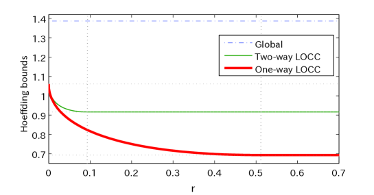
Figure 1: Comparison of Hoeffding bounds in one-way LOCC and two-way LOCC when $d=2$ and $\lambda=0.1$. In this case, we have $r_{\to}=0.511$, $r_{\leftrightarrow}=0.092$, $\log d_{A}d_{B}-H_{0}(\Psi)=0.693$, $\log d_{A}d_{B}-H_{1/2}(\Psi)=0.916$, and $\log d_{A}d_{B}-H_{1}(\Psi)=1.061$.

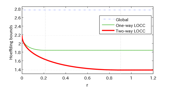
Figure 2: Comparison of Hoeffding bounds in one-way LOCC and two-way LOCC when $d=4$ and $\lambda=0.05$. In this case, we have $r_{\to}=0.911$, $r_{\leftrightarrow}=0.212$, $\log d_{A}d_{B}-H_{0}(\Psi)=1.386$, $\log d_{A}d_{B}-H_{1/2}(\Psi)=1.841$, and $\log d_{A}d_{B}-H_{1}(\Psi)=2.185$.

III Hypothesis testing under one-way LOCC POVMs

In this section, to show the relations for the one-way LOCC POVMs in Proposition 2 and Theorems 3 and 4 ((21), (24), and $\beta_{n,\rightarrow}\left(\epsilon|\Psi\|\rho_{mix}\right)=\max\{0,1-\bar{d}^{n}\epsilon\}$), we consider $C=\rightarrow$, that is, the local hypothesis testing under one-way LOCC POVMs. In this case, it turns out that our results can be formulated in terms of the following state

$$\sigma_{\Psi}\stackrel{{\scriptstyle\rm def}}{{=}}\sum_{i=1}^{d}\lambda_{i}|i\rangle\langle i|\otimes|i\rangle\langle i|,$$ (29)

where $\left\{|i\rangle\otimes|j\rangle\right\}_{i,j}$ is the Schmidt basis of $|\Psi\rangle$ [see Eq.(8)]. Then, our hypothesis testing is reduced to that with states $\sigma_{\Psi}$ and $\rho_{mix}$. That is, the last paper [56] showed the following lemma:

Proposition 6

Lemma 1 of [56] For all $\alpha>0$, we have

$$\beta_{n,\rightarrow}(\alpha|\Psi\|\rho_{mix}) =\beta_{n}(\alpha|\sigma_{\Psi}\|\rho_{mix}),$$ (30)

where the optimal type-2 error probability $\beta_{n,\rightarrow}(\alpha|\rho\|\sigma)$ is defined by Eq. (10). $\square$

Proofs of (24) and (21):   Since

$$D(\Psi\|\rho_{mix}) =\log d_{A}d_{B}-H_{1}(\Psi),\quad V(\Psi\|\rho_{mix})=V(\Psi),$$ (31)

$$\psi(s|\rho_{mix}\|\Psi) =(1-s)(H_{s}(\Psi)-\log d_{A}d_{B}),$$ (32)

by applying (6) to the commutative states $\rho=\rho_{mix}$ and $\sigma=\sigma_{\Psi}$, Proposition 6 yields (24). Similarly, applying (5), Proposition 6 reproduces the existing result (21). Therefore, we obtain the results for the one-way LOCC case.   

Proof of $\beta_{n,\rightarrow}\left(\epsilon|\Psi\|\rho_{mix}\right)=\max\{0,1-\bar{d}^{n}\epsilon\}$:   For the two hypotheses $\sigma_{\Psi}$ and $\rho_{mix}$, the optimal test $T$ has the support in the $n$-tensor product space of the subspace spanned by $\{|ii\rangle\}_{i=1}^{d}$ when $\epsilon\leq\frac{1}{\bar{d}^{n}}$. In this case, when $\mathrm{Tr}(I^{n}-T_{n})\rho_{mix}^{\otimes n}=\epsilon$, we have $\mathrm{Tr}(I^{n}-T_{n})\sigma_{\Psi}^{\otimes n}=\bar{d}^{n}\epsilon$. So, we obtain $\beta_{n,\rightarrow}\left(\epsilon|\Psi\|\rho_{mix}\right)=1-\bar{d}^{n}\epsilon$   

IV Hypothesis testing under separable POVM

IV-A Uniform case: Proof of Theorem 4

First, we consider the most simple case when the Schmidt coefficient is uniform, i.e., $\sqrt{\frac{1}{d^{n}}}$ because $d=\min(d_{A},d_{B})$. Then, for any separable POVM $\{T_{n},I^{n}-T_{n}\}$, we have[10]

$$\mathrm{Tr}T_{n}|\Psi\rangle\langle\Psi|\leq\frac{1}{d^{n}}\mathrm{Tr}T_{n}=d^{n}\mathrm{Tr}T_{n}\rho_{mix}.$$ (33)

Hence, when the first kind of error probability is restricted to $\mathrm{Tr}T_{n}|\Psi\rangle\langle\Psi|=\epsilon$, the second kind of error probability is evaluated as $\mathrm{Tr}(I^{n}-T_{n})\rho_{mix}\geq 1-\bar{d}\epsilon$. Hence, we have

$$\beta_{n,sep}\left(\epsilon|\Psi\|\rho_{mix}\right)\geq\max\{0,1-\bar{d}\epsilon\}$$ (34)

Since this lower bound can be attained by one-way LOCC, as mentioned in Section III, we obtain (26).

IV-B Hypothesis testing with a composite hypothesis: Proof of Theorem 5

In this subsection, in order to consider hypothesis testing under separable POVM for a pure state with the Schmidt decomposition $\sum_{i=1}^{d}\sqrt{p_{i}}|i\rangle\otimes|i\rangle$, we consider a pure state $|\varphi\rangle\stackrel{{\scriptstyle\rm def}}{{=}}\sum_{i=1}^{d}\sqrt{p_{i}}|i\rangle\in\mathbb{C}^{d}$ and a specific composite hypothesis testing on $(\mathbb{C}^{d})^{\otimes n}$ by employing the results in [66]. Here, we assume that $p_{1}\geq p_{2}\geq\ldots\geq p_{d}$.

IV-B1 Single-shot setting

Although our problem is based on $n$-fold setting, it is quite hard to find the relation between our problem and the results in [66]. To reduce the difficulty, we firstly discuss this relation with the single-shot setting. That is, in this subsubsection, we consider this specific composite hypothesis testing with the single-shot setting. Here, we assume that the distribution $p=(p_{i})$ is not uniform due to the assumption of Theorem 3. The following type of composite hypothesis testing plays a key role in our analysis of our hypothesis testing in the bipartite system. The null hypothesis is given as the pure state $|\varphi\rangle$ in the system $\mathbb{C}^{d}$. To give the alternative hypothesis, we introduce a notation. In the quantum system $\mathbb{C}^{d}$, the basis is written as $|j\rangle$ by using $j\in\{1,\ldots,d\}$. Hence, the quantum system $\mathbb{C}^{d}$ is spanned by $\{|j\rangle\}_{j\in{\cal D}}$, where ${\cal D}\stackrel{{\scriptstyle\rm def}}{{=}}\{1,\ldots,d\}$. Then, the alternative hypothesis ${\cal S}_{0}$ is the set of states $\left\{|\phi_{L}\rangle\right\}_{L\in\mathbb{Z}^{d}_{2}}$, where $|\phi_{L}\rangle\in\mathbb{C}^{d}$ is defined as

$$|\phi_{L}\rangle\stackrel{{\scriptstyle\rm def}}{{=}}\sqrt{\frac{1}{d}}\sum_{j\in{\cal D}}(-1)^{L_{j}}|j\rangle,\quad L\in\mathbb{Z}_{2}^{d},$$ (35)

where $L_{j}\in\mathbb{Z}_{2}$ is the $j$th entry of $L\in\mathbb{Z}_{2}^{d}$. That is, an element of the alternative hypothesis is characterized by an element of $\mathbb{Z}_{2}^{d}$. Hence, the cardinality of the alternative hypothesis is $2^{d}$.

For a two-valued POVM $\{S,I-S\}$ on $\mathbb{C}^{d}$, the type-1 error $\alpha(S)$ and type-2 error $\beta(S)$ are defined as

$$\alpha(S) \stackrel{{\scriptstyle\rm def}}{{=}}\mathrm{Tr}S|\varphi\rangle\langle\varphi|$$ (36)

$$\beta(S) \stackrel{{\scriptstyle\rm def}}{{=}}\max_{\rho\in{\cal S}_{0}}\mathrm{Tr}(I_{d}-S)\rho,$$ (37)

where $I_{d}$ is an identity operator on $\mathbb{C}^{d}$. The optimal type-2 error under the restriction on the condition that the type-1 error is no more than $\alpha\geq 0$ can be written as

$$\beta(\alpha|\varphi)\stackrel{{\scriptstyle\rm def}}{{=}}\min_{0\leq S\leq I_{d}}\{\beta(S)|\alpha(S)\leq\alpha\}.$$ (38)

Similarly, we define $\alpha(\beta|\varphi)$ as

$$\alpha(\beta|\varphi)\stackrel{{\scriptstyle\rm def}}{{=}}\min_{0\leq S\leq I_{d}}\{\alpha(S)|\beta(S)\leq\beta\}.$$ (39)

In the rest of this subsection, we often abbreviate $\beta(\alpha|\varphi)$ as $\beta\left(\alpha\right)$.

Now, we define the subset $S(R)\stackrel{{\scriptstyle\rm def}}{{=}}\{j\in{\cal D}|\log p_{j}\geq R\}$ of ${\cal D}$. We also employ the following notations:

$$P_{s}(R)\stackrel{{\scriptstyle\rm def}}{{=}} \sum_{j\in S(R)}(p_{j})^{s}\hbox{ for }s=0,1/2,1,$$ (40)

$$\epsilon(R)\stackrel{{\scriptstyle\rm def}}{{=}} \Big{(}\frac{P_{1/2}(R)^{2}}{dP_{1}(R)}\Big{)}^{\frac{1}{2}}.$$ (41)

When

$$1\geq\frac{P_{1/2}(\hat{R})^{2}}{P_{0}(R)P_{1}(\hat{R})},$$ (42)

we define

$$a(R,\hat{R})$$

$$\stackrel{{\scriptstyle\rm def}}{{=}} 1-P_{1}({R})\Biggl{(}\frac{P_{1/2}(R)P_{1/2}(\hat{R})}{P_{1}(\hat{R})^{\frac{1}{2}}P_{1}(R)^{\frac{1}{2}}P_{0}(R)}+\Bigl{(}1-\frac{P_{1/2}(\hat{R})^{2}}{P_{1}(\hat{R})P_{0}(R)}\Bigr{)}^{\frac{1}{2}}\Bigl{(}1-\frac{P_{1/2}(R)^{2}}{P_{1}(R)P_{0}(R)}\Bigr{)}^{\frac{1}{2}}\Biggr{)}^{2}.$$ (43)

Then, we have the following lemma.

Lemma 7

When the inequality $\epsilon(R)\geq\epsilon(\hat{R})$ holds, the condition (42) holds. $\square$

Proof: Since Schwarz inequality implies that $P_{0}(R)\geq\frac{P_{1/2}(R)^{2}}{P_{1}(R)}$, which implies the condition (42).   

Lemma 35 in Appendix B yields the following lemma.

Lemma 8

Any two distinct elements $R$ and $\hat{R}$ of $\{\log p_{i}\}_{i}$ with $R>\hat{R}$ satisfy the inequality $\epsilon(\hat{R})>\epsilon({R})$. $\square$

So, we have the following lemma.

Lemma 9

We fix $\hat{R}\in\{\log p_{i}\}_{i}$. Then, we have the following items.

(1)

When a real number $R(\in\{\log p_{i}\}_{i})<\hat{R}$ satisfies

$$\frac{P_{0}(R)}{P_{1/2}(R)}e^{\frac{R}{2}} \geq 1-\frac{\Bigl{(}\frac{P_{1}(R)P_{0}(R)}{P_{1/2}(R)^{2}}-1\Bigr{)}^{\frac{1}{2}}}{\Bigl{(}\frac{P_{1}(\hat{R})P_{0}(R)}{P_{1/2}(\hat{R})^{2}}-1\Bigr{)}^{\frac{1}{2}}},$$ (44)

we have

$$\alpha\left(\left.\frac{P_{1/2}(\hat{R})^{2}}{dP_{1}(\hat{R})}\right|\varphi\right)\leq a(R,\hat{R}).$$ (45)

(2)

We assume that there exists an element $R_{\alpha}$ in $\{\log p_{i}\}_{i}$ satisfying the inequality (44) and $R_{\alpha}<\hat{R}$. We denote all of distinct elements of $\{\log p_{i}\}_{i}$ by $\tilde{R}_{k}<\tilde{R}_{k-1}<\ldots<\tilde{R}_{2}<\tilde{R}_{1}$. We also assume that an element $R_{\beta}$ in $\{\log p_{i}\}_{i}$ satisfying the following condition; Any element $\tilde{R}_{j}(\leq R_{\beta})\in\{\log p_{i}\}_{i}$ satisfies

$$\frac{P_{0}(\tilde{R}_{j+1})}{P_{1/2}(\tilde{R}_{j})}e^{\frac{\tilde{R}_{j}}{2}} <1-\frac{\Bigl{(}\frac{P_{1}(\tilde{R}_{j+1})P_{0}(\tilde{R}_{j+1})}{P_{1/2}(\tilde{R}_{j})^{2}}-1\Bigr{)}^{\frac{1}{2}}}{\Bigl{(}\frac{P_{1}(\hat{R})P_{0}(\tilde{R}_{j})}{P_{1/2}(\hat{R})^{2}}-1\Bigr{)}^{\frac{1}{2}}}.$$ (46)

Then, the real numbers $\hat{R}$ and $R_{\beta}$ satisfy the inequality

$$\alpha\left(\left.\frac{P_{1/2}(\hat{R})^{2}}{dP_{1}(\hat{R})}\right|\varphi\right)\geq a(R_{\beta},\hat{R}).$$ (47)

$\square$

Proof of Lemma 8:   Here, we employ notations summarized in Appendix A. That is, we define the real vectors $u_{l}$ and $v_{l}$ on $\mathbb{R}^{l}$ as $u_{l}\stackrel{{\scriptstyle\rm def}}{{=}}\left(\sqrt{p_{1}},\cdots,\sqrt{p_{l}}\right)$ and $v_{l}\stackrel{{\scriptstyle\rm def}}{{=}}\left(1,\cdots,1\right)/\sqrt{d}$ for an integer $l$ satisfying $1\leq l\leq d$. We consider only the case when

$$l:=|S(R)|=P_{0}(R),\quad\hat{l}:=P_{0}(\hat{R}),\quad\epsilon^{2}:=\epsilon(\hat{R})^{2}=(\frac{u_{\hat{l}}\cdot v_{\hat{l}}}{\|u_{\hat{l}}\|})^{2}=\frac{P_{1/2}(\hat{R})^{2}}{dP_{1}(\hat{R})}.$$ (48)

Since $R$ and $\hat{R}$ are two distinct elements of $\{\log p_{i}\}_{i}$ and $R>\hat{R}$, we have the inequality $l<\hat{l}$. Due to the above final relation, Lemma 35 in Appendix B directly implies Lemma 8.   

Proof of Lemma 9:   We prove Lemma 9 by using the notations in the above proof of Lemma 8. For this purpose, we employ results in [66], which are summarized in Appendix A. Due to (48), we have

$$u_{l}\cdot v_{l}=\frac{P_{1/2}(R)}{d^{1/2}},\quad\|v_{l}\|^{2}=\frac{P_{0}(R)}{d},\quad\|u_{l}\|^{2}=P_{1}(R).$$ (49)

Since $R<\hat{R}$, we have $l\geq\hat{l}$.

Item (1):  Firstly, we show Item (1) by using the properties of ${x}^{*}(u_{l},v_{l},\epsilon)$ given in Proposition 31. That is, we show (45) by assuming (44). Since $R<\hat{R}$, Lemma 8 guarantees that $\frac{u_{l}\cdot v_{l}}{\|u_{l}\|}=\epsilon(R)>\epsilon(\hat{R})=\epsilon$, which implies (42) by using Lemma 7. Hence, the vector ${x}^{*}(u_{l},v_{l},\epsilon)$ defined in (264) of Proposition 31 in Appendix A is written as

$${x}^{*}(u_{l},v_{l},\epsilon)$$

$$= \frac{1}{\sqrt{\|u_{l}\|^{2}\|v_{l}\|^{2}-(u_{l}\cdot v_{l})^{2}}}\bigg{(}\sqrt{\|v_{l}\|^{2}-\epsilon^{2}}u_{l}$$

$$\hskip 99.02747pt+\frac{\epsilon\sqrt{\|u_{l}\|^{2}\|v_{l}\|^{2}-(u_{l}\cdot v_{l})^{2}}-u_{l}\cdot v_{l}\sqrt{\|v_{l}\|^{2}-\epsilon^{2}}}{\|v_{l}\|^{2}}v_{l}\bigg{)}.$$ (50)

Due to Lemma 36 in Appendix B, all entries of ${x}^{*}(u_{l},v_{l},\epsilon)$ are non-negative if and only if

$$\sqrt{p_{l}}\frac{d^{1/2}\|v_{l}\|^{2}}{u_{l}\cdot v_{l}}\geq\left(1-\frac{\sqrt{\frac{\|u_{l}\|^{2}\|v_{l}\|^{2}}{(u_{l}\cdot v_{l})^{2}}-1}}{\sqrt{\frac{\|v_{l}\|^{2}}{\epsilon^{2}}-1}}\right),$$ (51)

which is equivalent to (44), due to the relations (48) and (49). So, all entries of ${x}^{*}(u_{l},v_{l},\epsilon)$ are non-negative. Thus, for any $L\in\mathbb{Z}_{2}^{d}$, we find that

$$\langle x^{*}(u_{l},v_{l},\epsilon)|\phi_{L}\rangle^{2}\stackrel{{\scriptstyle(a)}}{{\leq}}\Big{\langle}x^{*}(u_{l},v_{l},\epsilon)\Big{|}\sum_{i=1}^{d}\frac{1}{\sqrt{d}}\Big{|}i\Big{\rangle}^{2}\stackrel{{\scriptstyle(b)}}{{=}}\langle x^{*}(u_{l},v_{l},\epsilon)|v_{l}\rangle^{2}\stackrel{{\scriptstyle(c)}}{{\leq}}\epsilon^{2},$$ (52)

where $(a)$, $(b)$, and $(c)$ follow from the non-negativity of all entries of $x^{*}(u_{l},v_{l},\epsilon)$, the equations (50), and the property of ${x}^{*}(u_{l},v_{l},\epsilon)$ given in Proposition 31, respectively. Thus, since $|\varphi\rangle=u_{d}$, using (50) and (52), we have

$$1-\alpha\left(\left.\epsilon^{2}\right|\varphi\right)\stackrel{{\scriptstyle(a)}}{{\geq}}\langle\varphi|x^{*}(u_{l},v_{l},\epsilon)\rangle^{2}$$

$$\stackrel{{\scriptstyle(b)}}{{=}} \frac{(u_{l}\cdot v_{l}\epsilon+\sqrt{(\|v_{l}\|^{2}-\epsilon^{2})(\|v_{l}\|^{2}\|u_{l}\|^{2}-(u_{l}\cdot v_{l})^{2})})^{2}}{\|v_{l}\|^{4}}$$

$$\stackrel{{\scriptstyle(c)}}{{=}} \frac{\left(\frac{P_{1/2}(R)}{d^{1/2}}\frac{P_{1/2}(\hat{R})}{d^{1/2}P_{1}(\hat{R})^{1/2}}+\sqrt{(\frac{P_{0}(R)}{d}-\frac{P_{1/2}(\hat{R})^{2}}{dP_{1}(\hat{R})})(\frac{P_{0}(R)P_{1}(R)}{d}-\frac{P_{1/2}(R)^{2}}{d})}\right)^{2}}{\frac{P_{0}(R)^{2}}{d^{2}}}$$

$$= P_{1}({R})\Biggl{(}\frac{P_{1/2}(R)P_{1/2}(\hat{R})}{P_{1}(\hat{R})^{\frac{1}{2}}P_{1}(R)^{\frac{1}{2}}P_{0}(R)}+\Bigl{(}1-\frac{P_{1/2}(\hat{R})^{2}}{P_{1}(\hat{R})P_{0}(R)}\Bigr{)}^{\frac{1}{2}}\Bigl{(}1-\frac{P_{1/2}(R)^{2}}{P_{1}(R)P_{0}(R)}\Bigr{)}^{\frac{1}{2}}\Biggr{)}^{2},$$ (53)

where $(a)$, $(b)$, and $(c)$ follow from (52), (50) with $|\varphi\rangle=u_{d}$, and (49), respectively. So, we obtain the inequality (45).

Item (2):  Step 1:) Next, we proceed to the proof of Item (2) by combining Propositions 31 and 33. That is, we will show (47) by assuming (46). Now, we outline the derivation of (47). For the preparation, we choose $l_{\beta}:=|S(R_{\beta})|=P_{0}(R_{\beta})$, $\hat{l}:=|S(\hat{R})|=P_{0}(\hat{R})$, $l_{\alpha}:=|S(R_{\alpha})|=P_{0}(R_{\alpha})$, $\epsilon:=\epsilon(\hat{R})=\frac{u_{\hat{l}}\cdot v_{\hat{l}}}{\|u_{\hat{l}}\|}$, and $\eta:=\eta_{\epsilon}$, where $\eta_{\epsilon}$ is defined in Appendix A. In Step 2:), we show the inequality $l_{\beta}>\eta$. In Step 3:), we show

$$1-\alpha\left(\left.\epsilon^{2}\right|\varphi\right)=\frac{\Big{(}u_{\eta}\cdot v_{\eta}\epsilon+\sqrt{(\|v_{\eta}\|^{2}-\epsilon^{2})(\|v_{\eta}\|^{2}\|u_{\eta}\|^{2}-(u_{\eta}\cdot v_{\eta})^{2})}\Big{)}^{2}}{\|v_{\eta}\|^{4}},$$ (54)

and

$$\max\{\langle u_{l_{\beta}}|\phi\rangle^{2}||\phi\rangle\in\mathbb{R}^{l_{\beta}},\|\phi\|^{2}=1,\langle v_{l_{\beta}}|\phi\rangle\leq\epsilon\}$$

$$= \frac{\Big{(}u_{l_{\beta}}\cdot v_{l_{\beta}}\epsilon+\sqrt{(\|v_{l_{\beta}}\|^{2}-\epsilon^{2})(\|v_{l_{\beta}}\|^{2}\|u_{l_{\beta}}\|^{2}-(u_{l_{\beta}}\cdot v_{l_{\beta}})^{2})}\Big{)}^{2}}{\|v_{l_{\beta}}\|^{4}}.$$ (55)

In Step 4:), combining these relations, we show the inequality (47).

Step 2:) Firstly, we show that the condition A1), A2), nor A3) in Appendix A does not hold for any integer $l$ satisfying $l\geq l_{\beta}$. Due to Lemma 34, A2) does not hold because $R_{\beta}<\log p_{1}$. Since $l_{\beta}>\hat{l}$, Lemma 35 guarantees that A1) does not hold for any integer $l$ satisfying $l\geq l_{\beta}$.

Now, to show the inequality $l_{\beta}>\eta$, we show that A3) does not hold for any integer $l$ satisfying $l\geq l_{\beta}$. We choose $\tilde{l}_{j}:=|S(\tilde{R}_{j})|=P_{0}(\tilde{R}_{j})$. For a given integer $l\geq l_{\beta}$, we choose $j$ such that $\tilde{l}_{j+1}>l\geq\tilde{l}_{j}$, which implies the relations

$$p_{l}\leq p_{\tilde{l}_{j}},~{}\|v_{\tilde{l}_{j}}\|\leq\|v_{l}\|\leq\|v_{\tilde{l}_{j+1}}\|,~{}\|u_{l}\|\leq\|u_{\tilde{l}_{j+1}}\|,~{}u_{\tilde{l}_{j}}\cdot v_{\tilde{l}_{j}}.\leq u_{l}\cdot v_{l}\leq u_{\tilde{l}_{j+1}}\cdot v_{\tilde{l}_{j+1}}.$$ (56)

Then, we have

$$\sqrt{p_{l}}\frac{d^{1/2}\|v_{l}\|^{2}}{u_{l}\cdot v_{l}}\stackrel{{\scriptstyle(a)}}{{\leq}}\sqrt{p_{\tilde{l}_{j}}}\frac{d^{1/2}\|v_{\tilde{l}_{j+1}}\|^{2}}{u_{\tilde{l}_{j}}\cdot v_{\tilde{l}_{j}}}\stackrel{{\scriptstyle(b)}}{{<}}\left(1-\frac{\sqrt{\frac{\|u_{\tilde{l}_{j+1}}\|^{2}\|v_{\tilde{l}_{j+1}}\|^{2}}{(u_{\tilde{l}_{j}}\cdot v_{\tilde{l}_{j}})^{2}}-1}}{\sqrt{\frac{\|v_{\tilde{l}_{j}}\|^{2}}{\epsilon^{2}}-1}}\right)\stackrel{{\scriptstyle(c)}}{{\leq}}\left(1-\frac{\sqrt{\frac{\|u_{l}\|^{2}\|v_{l}\|^{2}}{(u_{l}\cdot v_{l})^{2}}-1}}{\sqrt{\frac{\|v_{l}\|^{2}}{\epsilon^{2}}-1}}\right),$$ (57)

where $(b)$ follows from the condition (46), and $(a)$ and $(c)$ follow from (56). This inequality shows that the condition (280) in Lemma 36 does not hold. Since Lemma 35 guarantees that $\frac{u_{l}\cdot v_{l}}{\|u_{l}\|}$ is strictly monotone increasing for $l$, we have $\frac{u_{l}\cdot v_{l}}{\|u_{l}\|}\geq\frac{u_{l_{\beta}}\cdot v_{l_{\beta}}}{\|u_{l_{\beta}}\|}>\frac{u_{\hat{l}}\cdot v_{\hat{l}}}{\|u_{\hat{l}}\|}=\epsilon$ because $l_{\beta}>\hat{l}$. By using these two statements, Lemma 36 guarantees that the ${l}$-th entry of $x^{*}(u_{{l}},v_{{l}},\epsilon)$ is negative for the integer $l$. So, A3) does not hold for any integer $l$ satisfying $l\geq l_{\beta}$. Thus, the assumption of Item (2) implies that neither A1), A2), nor A3) does not hold for any integer $l$ satisfying $l\geq l_{\beta}$. Hence, we have the desired inequality $l_{\beta}>\eta$.

Step 3:) Since $R_{\alpha}<\hat{R}$, Lemma 8 implies that $\frac{u_{l_{\alpha}}\cdot v_{l_{\alpha}}}{\|u_{l_{\alpha}}\|}=\epsilon(R_{\alpha})>\epsilon(\hat{R})=\epsilon$. Item (1) guarantees that $l_{\alpha}$ satisfies Condition A3). So, $\eta\geq l_{\alpha}$. Thus, Lemma 35 yields that $\frac{u_{\eta}\cdot v_{\eta}}{\|u_{\eta}\|}\geq\frac{u_{l_{\alpha}}\cdot v_{l_{\alpha}}}{\|u_{l_{\alpha}}\|}>\epsilon$. Hence, B1) does not hold. Since $R_{\alpha}<\hat{R}$ implies $R_{\alpha}<\log p_{1}$, we have $\log p_{\eta}\leq R_{\alpha}<\log p_{1}$. So, B2) does not hold due to Lemma 34. Thus, B3) holds. So, Proposition 33 guarantees (54), and the maximum $1-\alpha\left(\left.\epsilon^{2}\right|\varphi\right)$ in (54) is attained by the vector $x^{*}(u_{\eta},v_{\eta},\epsilon)$.

Then, we apply Proposition 31 to the case with $y=u_{l_{\beta}}$ and $z=v_{l_{\beta}}$. Since the condition D3), i.e., the relation $y/\|y\|\neq z/\|z\|$ and $y\cdot z>\epsilon\|y\|$ holds, we obtain (55).

Step 4:) We show the inequality (47). Since the inequality $l_{\beta}>\eta$ implies the equation $\langle v_{l_{\beta}}|x^{*}(u_{\eta},v_{\eta},\epsilon)\rangle=\langle v_{\eta}|x^{*}(u_{\eta},v_{\eta},\epsilon)\rangle$, we find that the vector $x^{*}(u_{\eta},v_{\eta},\epsilon)$ also satisfies the condition for the real vector $|\phi\rangle$ in the maximum in the LHS of (55). So, we have

$$\max\{\langle u_{l_{\beta}}|\phi\rangle^{2}||\phi\rangle\in\mathbb{R}^{l_{\beta}},\|\phi\|^{2}=1,\langle v_{l_{\beta}}|\phi\rangle\leq\epsilon\}$$

$$\geq \frac{\Big{(}u_{\eta}\cdot v_{\eta}\epsilon+\sqrt{(\|v_{\eta}\|^{2}-\epsilon^{2})(\|v_{\eta}\|^{2}\|u_{\eta}\|^{2}-(u_{\eta}\cdot v_{\eta})^{2})}\Big{)}^{2}}{\|v_{\eta}\|^{4}}.$$ (58)

Combining (54), (55), and (58), we have

$$1-\alpha\left(\left.\epsilon^{2}\right|\varphi\right)$$

$$\leq \frac{\Big{(}u_{l_{\beta}}\cdot v_{l_{\beta}}\epsilon+\sqrt{(\|v_{l_{\beta}}\|^{2}-\epsilon^{2})(\|v_{l_{\beta}}\|^{2}\|u_{l_{\beta}}\|^{2}-(u_{l_{\beta}}\cdot v_{l_{\beta}})^{2})}\Big{)}^{2}}{\|v_{l_{\beta}}\|^{4}}.$$ (59)

Hence, combining the same discussion as (53), we obtain the inequality (47).   

Note that it is quite difficult to derive the tight evaluation of $\alpha\left(\left.\frac{P_{1/2}(\hat{R})^{2}}{dP_{1}(\hat{R})}\right|\varphi\right)$ because our choice of $l$ is limited to $l=|S(R)|=P_{0}(R)$. We obtain lower and upper bounds as (45).

Using $P_{1}^{c}(R)\stackrel{{\scriptstyle\rm def}}{{=}}1-P_{1}(R)$, we have the following lemma.

Lemma 10

When $R<\hat{R}$, the number $a(R,\hat{R})$ is bounded as follows.

$$P_{1}^{c}(R)\leq a(R,\hat{R})\leq P_{1}^{c}(\hat{R}).$$ (60)

$\square$

Proof: To show Lemma 10, we will show the following.

$$P_{1}(\hat{R})\leq 1-a(R,\hat{R})\leq P_{1}(R).$$ (61)

First, we show the second inequality of (61). Since

$$\frac{P_{1/2}(\hat{R})^{2}}{P_{0}(R)P_{1}(\hat{R})}+\frac{P_{1/2}(R)^{2}}{P_{0}(R)P_{1}(R)}\geq 2\Big{(}\frac{P_{1/2}(\hat{R})^{2}}{P_{0}(R)P_{1}(\hat{R})}\cdot\frac{P_{1/2}(R)^{2}}{P_{0}(R)P_{1}(R)}\Big{)}^{\frac{1}{2}}$$

$$= 2\frac{P_{1/2}(R)P_{1/2}(\hat{R})}{P_{0}(R)P_{1}(R)^{\frac{1}{2}}P_{1}(\hat{R})^{\frac{1}{2}}},$$

we have

$$\Bigl{(}1-\frac{P_{1/2}(\hat{R})^{2}}{P_{0}(R)P_{1}(\hat{R})}\Bigr{)}\Bigl{(}1-\frac{P_{1/2}(R)^{2}}{P_{0}(R)P_{1}(R)}\Bigr{)}$$

$$\leq \Bigl{(}1-\frac{P_{1/2}(R)P_{1/2}(\hat{R})}{P_{0}(R)P_{1}(R)^{\frac{1}{2}}P_{1}(\hat{R})^{\frac{1}{2}}}\Bigr{)}^{2},$$

i.e.,

$$\Bigl{(}1-\frac{P_{1/2}(\hat{R})^{2}}{P_{0}(R)P_{1}(\hat{R})}\Bigr{)}^{\frac{1}{2}}\Bigl{(}1-\frac{P_{1/2}(R)^{2}}{P_{0}(R)P_{1}(R)}\Bigr{)}^{\frac{1}{2}}$$

$$\leq 1-\frac{P_{1/2}(R)P_{1/2}(\hat{R})}{P_{0}(R)P_{1}(R)^{\frac{1}{2}}P_{1}(\hat{R})^{\frac{1}{2}}}.$$

Therefore,

$$P_{1}(R)\Biggl{(}\frac{P_{1/2}(R)P_{1/2}(\hat{R})}{P_{0}(R)P_{1}(R)^{\frac{1}{2}}P_{1}(\hat{R})^{\frac{1}{2}}}$$

$$\hskip 77.49976pt+\Bigl{(}1-\frac{P_{1/2}(\hat{R})^{2}}{P_{0}(R)P_{1}(\hat{R})}\Bigr{)}^{\frac{1}{2}}\Bigl{(}1-\frac{P_{1/2}(R)^{2}}{P_{0}(R)P_{1}(R)}\Bigr{)}^{\frac{1}{2}}\Biggr{)}^{2}$$

$$\leq P_{1}(R)\Biggl{(}\frac{P_{1/2}(R)P_{1/2}(\hat{R})}{P_{0}(R)P_{1}(R)^{\frac{1}{2}}P_{1}(\hat{R})^{\frac{1}{2}}}+1-\frac{P_{1/2}(R)P_{1/2}(\hat{R})}{P_{0}(R)P_{1}(R)^{\frac{1}{2}}P_{1}(\hat{R})^{\frac{1}{2}}}\Biggr{)}^{2}$$

$$= P_{1}(R).$$

Then, we obtain the second inequality of (61).

To show the first inequality of (61), we employ the notation given in Appendix A, and choose the integers $l:=|S(R)|=P_{0}(R)$ and $\hat{l}:=|S(\hat{R})|=P_{0}(\hat{R})$ in the same way as the proof of Lemma 9. So, the condition $R<\hat{R}$ implies that $\hat{l}\leq l$. Hence, we have $\|u_{\hat{l}}\|^{2}=u_{l}\cdot u_{\hat{l}}$. We apply Proposition 31 to the case when $y=u_{l}$, $z=v_{l}$, and $\epsilon=\frac{u_{\hat{l}}\cdot v_{\hat{l}}}{\|u_{\hat{l}}\|}$. Then, we find that $x=\frac{u_{\hat{l}}}{\|u_{\hat{l}}\|}$ satisfies the condition in $M(u_{l},v_{l},\epsilon)$ given in (255).

Now, we show that

$$\|u_{\hat{l}}\|^{2}\leq\left(\frac{u_{l}\cdot v_{l}\epsilon+\sqrt{(\|v_{l}\|^{2}-\epsilon^{2})(\|v_{l}\|^{2}\|u_{l}\|^{2}-(u_{l}\cdot v_{l})^{2})}}{\|v_{l}\|^{2}}\right)^{2}.$$ (62)

When $l=\hat{l}$, the RHS of (62) equals $\|u_{\hat{l}}\|^{2}$. So, we show (62) when $l>\hat{l}$ as follows. In this case, Lemma 35 implies that $\frac{u_{l}\cdot v_{l}}{\|u_{l}\|}>\frac{u_{\hat{l}}\cdot v_{\hat{l}}}{\|u_{\hat{l}}\|}=\epsilon$. Proposition 31 with Case D3 guarantees that

$$\|u_{\hat{l}}\|=u_{l}\cdot\frac{u_{\hat{l}}}{\|u_{\hat{l}}\|}\leq\frac{u_{l}\cdot v_{l}\epsilon+\sqrt{(\|v_{l}\|^{2}-\epsilon^{2})(\|v_{l}\|^{2}\|u_{l}\|^{2}-(u_{l}\cdot v_{l})^{2})}}{\|v_{l}\|^{2}},$$ (63)

which implies (62).

Therefore,

$$P_{1}(\hat{R})=\|u_{\hat{l}}\|^{2}\leq\left(\frac{u_{l}\cdot v_{l}\epsilon+\sqrt{(\|v_{l}\|^{2}-\epsilon^{2})(\|v_{l}\|^{2}\|u_{l}\|^{2}-(u_{l}\cdot v_{l})^{2})}}{\|v_{l}\|^{2}}\right)^{2}$$

$$\stackrel{{\scriptstyle(a)}}{{=}} P_{1}({R})\Biggl{(}\frac{P_{1/2}(R)P_{1/2}(\hat{R})}{P_{1}(\hat{R})^{\frac{1}{2}}P_{1}(R)^{\frac{1}{2}}P_{0}(R)}+\Bigl{(}1-\frac{P_{1/2}(\hat{R})^{2}}{P_{1}(\hat{R})P_{0}(R)}\Bigr{)}^{\frac{1}{2}}\Bigl{(}1-\frac{P_{1/2}(R)^{2}}{P_{1}(R)P_{0}(R)}\Bigr{)}^{\frac{1}{2}}\Biggr{)}^{2}=1-a(R,\hat{R}),$$ (64)

where $(a)$ follows from (53). Then, we obtain the first inequality of (61).   

IV-B2 $n$-fold i.i.d. setting

In this subsection, we rewrite the results in the previous subsection in $n$-fold i.i.d. setting. In this setting, The null hypothesis is given as the pure state $|\varphi^{\otimes n}\rangle$ in the $n$-tensor product system $(\mathbb{C}^{d})^{\otimes n}$. To give the alternative hypothesis, we introduce a notation. In the quantum system $(\mathbb{C}^{d})^{\otimes n}$, the basis $|i_{1}\rangle\otimes\cdots\otimes|i_{n}\rangle$ is simplified to $|J\rangle$ by using $J\in\{1,\ldots,d\}^{n}$. Hence, the quantum system $(\mathbb{C}^{d})^{\otimes n}$ is spanned by $\{|J\rangle\}_{J\in{\cal D}^{n}}=\{|i_{1}\rangle\otimes\cdots\otimes|i_{n}\rangle\}_{i_{1},\dots,i_{n}}$, where ${\cal D}^{n}\stackrel{{\scriptstyle\rm def}}{{=}}\{1,\ldots,d\}^{n}$. Then, the alternative hypothesis ${\cal S}_{n,0}$ is the set of states $\left\{|\phi_{L}^{n}\rangle\right\}_{L\in\mathbb{Z}^{d^{n}}_{2}}$, where $|\phi_{L}^{n}\rangle\in\left(\mathbb{C}^{d}\right)^{\otimes n}$ is defined as

$$|\phi_{L}^{n}\rangle\stackrel{{\scriptstyle\rm def}}{{=}}\sqrt{\frac{1}{d^{n}}}\sum_{J\in{\cal D}^{n}}(-1)^{L_{J}}|J\rangle,\quad L\in\mathbb{Z}_{2}^{d^{n}},$$ (65)

where $L_{J}\in\mathbb{Z}_{2}$ is the $J$th entry of $L\in\mathbb{Z}_{2}^{d^{n}}$. That is, an element of the alternative hypothesis is characterized by an element of $\mathbb{Z}_{2}^{d^{n}}$. Hence, the cardinality of the alternative hypothesis is $2^{d^{n}}$, which is double exponential with respect to the number $n$.

For a two-valued POVM $\{S_{n},I_{d}^{n}-S_{n}\}$ on $\left(\mathbb{C}^{d}\right)^{\otimes n}$, the type-1 error $\alpha_{n}(S_{n})$ and type-2 error $\beta_{n}(S_{n})$ are defined as

$$\alpha_{n}(S_{n}) \stackrel{{\scriptstyle\rm def}}{{=}}\mathrm{Tr}S_{n}|\varphi\rangle\langle\varphi|^{\otimes n}$$ (66)

$$\beta_{n}(S_{n}) \stackrel{{\scriptstyle\rm def}}{{=}}\max_{\rho\in{\cal S}_{n,0}}\mathrm{Tr}(I_{d}^{n}-S_{n})\rho,$$ (67)

where $I_{d}^{n}$ is an identity operator on $(\mathbb{C}^{d})^{\otimes n}$. The optimal type-2 error under the restriction on the condition that the type-1 error is no more than $\alpha\geq 0$ can be written as

$$\beta_{n}(\alpha|\varphi)\stackrel{{\scriptstyle\rm def}}{{=}}\min_{0\leq S_{n}\leq I_{d}^{n}}\{\beta_{n}(S_{n})|\alpha_{n}(S_{n})\leq\alpha\}.$$ (68)

Similarly, we define $\alpha_{n}(\beta|\varphi)$ as

$$\alpha_{n}(\beta|\varphi)\stackrel{{\scriptstyle\rm def}}{{=}}\min_{0\leq S_{n}\leq I_{d}^{n}}\{\alpha_{n}(S_{n})|\beta_{n}(S_{n})\leq\beta\}.$$ (69)

In the rest of this subsection, we often abbreviate $\beta_{n}(\alpha|\varphi)$ as $\beta_{n}\left(\alpha\right)$.

Now, we define the subset $S_{n}(R)\stackrel{{\scriptstyle\rm def}}{{=}}\{J\in{\cal D}^{n}|\log p^{n}_{J}\geq nR\}$ of ${\cal D}^{n}$, where $p^{n}_{J}\stackrel{{\scriptstyle\rm def}}{{=}}p_{i_{1}}\cdots p_{i_{n}}$ for $J=(i_{1},\ldots,i_{n})$. We employ the following notations:

$$P_{n,s}(R)\stackrel{{\scriptstyle\rm def}}{{=}} \sum_{J\in S_{n}(R)}(p^{n}_{J})^{s}\hbox{ for }s=0,1/2,1,$$

$$\epsilon_{n}(R)\stackrel{{\scriptstyle\rm def}}{{=}} \Big{(}\frac{P_{n,1/2}(R)^{2}}{d^{n}P_{n,1}(R)}\Big{)}^{\frac{1}{2}}.$$

When

$$1\geq\frac{P_{n,1/2}(\hat{R})^{2}}{P_{n,0}(R)P_{n,1}(\hat{R})},$$ (70)

we define

$$a_{n}(R,\hat{R})$$

$$\stackrel{{\scriptstyle\rm def}}{{=}} 1-P_{n,1}({R})\Biggl{(}\frac{P_{n,1/2}(R)P_{n,1/2}(\hat{R})}{P_{n,1}(\hat{R})^{\frac{1}{2}}P_{n,1}(R)^{\frac{1}{2}}P_{n,0}(R)}+\Bigl{(}1-\frac{P_{n,1/2}(\hat{R})^{2}}{P_{n,1}(\hat{R})P_{n,0}(R)}\Bigr{)}^{\frac{1}{2}}\Bigl{(}1-\frac{P_{n,1/2}(R)^{2}}{P_{n,1}(R)P_{n,0}(R)}\Bigr{)}^{\frac{1}{2}}\Biggr{)}^{2}.$$ (71)

Then, Lemmas 9 and 10 are rewritten as follows.

Lemma 11

We fix $\hat{R}\in\{\frac{1}{n}\log p_{J}^{n}\}_{J\in{\cal D}^{n}}$. Then, we have the following items.

(1)

When a real number $R(\in\{\frac{1}{n}\log p_{J}^{n}\}_{J\in{\cal D}^{n}})<\hat{R}$ satisfies

$$\frac{P_{n,0}(R)}{P_{n,1/2}(R)}e^{\frac{nR}{2}}+\frac{\Bigl{(}\frac{P_{n,1}(R)P_{n,0}(R)}{P_{n,1/2}(R)^{2}}-1\Bigr{)}^{\frac{1}{2}}}{\Bigl{(}\frac{P_{n,1}(\hat{R})P_{n,0}(R)}{P_{n,1/2}(\hat{R})^{2}}-1\Bigr{)}^{\frac{1}{2}}}\geq 1,$$ (72)

we have

$$\alpha_{n}\left(\left.\frac{P_{n,1/2}(\hat{R})^{2}}{d^{n}P_{n,1}(\hat{R})}\right|\varphi\right)\leq a_{n}(R,\hat{R}).$$ (73)

(2)

We assume that there exists an element $R_{\alpha}$ in $\{\frac{1}{n}\log p_{J}^{n}\}_{J\in{\cal D}^{n}}$ satisfying the inequality (72) and $R_{\alpha}<\hat{R}$. We denote all of distinct elements of $\{\frac{1}{n}\log p_{J}^{n}\}_{J\in{\cal D}^{n}}$ by $\tilde{R}_{k}<\tilde{R}_{k-1}<\ldots<\tilde{R}_{2}<\tilde{R}_{1}$. We also assume that an element $R_{\beta}$ in $\{\frac{1}{n}\log p_{J}^{n}\}_{J\in{\cal D}^{n}}$ satisfying the following condition; Any element $\tilde{R}_{j}(\leq R_{\beta})\in\{\frac{1}{n}\log p_{J}^{n}\}_{J\in{\cal D}^{n}}$ satisfies

$$\frac{P_{n,0}(\tilde{R}_{j+1})}{P_{n,1/2}(\tilde{R}_{j})}e^{\frac{\tilde{R}_{j}}{2}}+\frac{\Bigl{(}\frac{P_{n,1}(\tilde{R}_{j+1})P_{n,0}(\tilde{R}_{j+1})}{P_{n,1/2}(\tilde{R}_{j})^{2}}-1\Bigr{)}^{\frac{1}{2}}}{\Bigl{(}\frac{P_{n,1}(\hat{R})P_{n,0}(\tilde{R}_{j})}{P_{n,1/2}(\hat{R})^{2}}-1\Bigr{)}^{\frac{1}{2}}}<1.$$ (74)

Then, the real numbers $\hat{R}$ and $R_{\beta}$ satisfy the inequality

$$\alpha_{n}\left(\left.\frac{P_{n,1/2}(\hat{R})^{2}}{d^{n}P_{n,1}(\hat{R})}\right|\varphi\right)\geq a_{n}(R_{\beta},\hat{R}).$$ (75)

$\square$

Lemma 12

When $R<\hat{R}$, the number $a_{n}(R,\hat{R})$ is evaluated as

$$P_{n,1}^{c}(R)\leq a_{n}(R,\hat{R})\leq P_{n,1}^{c}(\hat{R}),$$ (76)

where $P_{n,1}^{c}(R)\stackrel{{\scriptstyle\rm def}}{{=}}1-P_{n,1}(R)$. $\square$

IV-B3 Constant constraint for type-1 error

Under a constant constraint for type-1 error, we have the following theorem.

Theorem 13

We have

$$\log\beta_{n}(\epsilon|\varphi)= n(H(p)-\log d)-\sqrt{n}\sqrt{V(p)}\Phi^{-1}(\epsilon)-\log n+O(1),$$ (77)

where $H(p)\stackrel{{\scriptstyle\rm def}}{{=}}-\sum_{i}p_{i}\log p_{i}$ and $V(p)\stackrel{{\scriptstyle\rm def}}{{=}}\sum_{i}p_{i}(H(p)+\log p_{i})^{2}$. $\square$

For a preparation of the proof of Theorem 13, we introduce several notations. First, we choose $A_{\epsilon}\stackrel{{\scriptstyle\rm def}}{{=}}\sqrt{V(p)}\Phi^{-1}(\epsilon)$. Remember that $\Phi$ is the cumulative distribution function of the standard Gaussian distribution. We fix $d_{S}$ to be the lattice span of the random variable $-\log p_{I}$ when the index $I$ is subject to the distribution $p$. Hence, the set $\{\frac{1}{n}\log p_{J}^{n}\}_{J\in{\cal D}^{n}}$ has the lattice structure with the span $\frac{d_{S}}{n}$. For the precise definition of $d_{S}$, see Appendix C. Then, we define the functions $g_{1}$, $g_{2}$, and $g_{3}$ as

$$g_{1}(d_{S}) :=\left\{\begin{array}[]{ll}-\log 2&\hbox{ if }d_{S}=0\\ \log\frac{1-e^{-\frac{1}{2}d_{S}}}{1-e^{-d_{S}}}&\hbox{ if }d_{S}>0,\end{array}\right.$$ (80)

$$g_{2}(d_{S}) :=\left\{\begin{array}[]{ll}-\frac{1}{2}\log 2\pi+\frac{1}{2V(p)}+2\log 2&\hbox{ if }d_{S}=0\\ -\frac{1}{2}\log 2\pi+\frac{1}{2V(p)}+\log\frac{1-e^{-d_{S}}}{(1-e^{-\frac{1}{2}d_{S}})^{2}}&\hbox{ if }d_{S}>0,\end{array}\right.$$ (83)

$$g_{3}(d_{S}) :=\left\{\begin{array}[]{ll}-\frac{1}{2}\log 2\pi+\log 2+\frac{1}{2V(p)}&\hbox{ if }d_{S}=0\\ -\frac{1}{2}\log 2\pi+\frac{1}{2V(p)}+\log\frac{d_{S}}{1-e^{-\frac{1}{2}d_{S}}}&\hbox{ if }d_{S}>0.\end{array}\right.$$ (86)

Then, we have the following lemma, which will be shown after the proof of Theorem 13.

Lemma 14

For real numbers $B_{i}$ with $i=1,2,3,4,5$, we define ${R}_{n,i}\stackrel{{\scriptstyle\rm def}}{{=}}-H(p)+\frac{A_{\epsilon}}{\sqrt{n}}+\frac{B_{i}}{n}$ with $i=1,2,3,4,5$.

$$\log\frac{P_{n,1/2}(R_{n,1})P_{n,1/2}(R_{n,2})}{P_{n,1}(R_{n,3})^{\frac{1}{2}}P_{n,1}(R_{n,4})^{\frac{1}{2}}P_{n,0}(R_{n,5})}=-\frac{1}{2}\log n+B_{5}-\frac{B_{3}+B_{4}}{2}+g_{2}(d_{S})-\log(1-\epsilon)+o(1).$$ (87)

The convergences of the differences between the LHSs and RHSs are compact uniform for $B_{i}$.

Assume that $\hat{R}_{n}:=-H(p)+\frac{A_{\epsilon}}{\sqrt{n}}+\frac{\hat{B}_{n}}{n}$, $R_{n}=-H(p)+\frac{A_{\epsilon}}{\sqrt{n}}+\frac{B_{n}}{n}$, and $R_{n}^{\prime}=-H(p)+\frac{A_{\epsilon}}{\sqrt{n}}+\frac{B_{n}^{\prime}}{n}$.

When $B_{n}$ and $\hat{B}_{n}$ are bounded, and $B_{n}-B_{n}^{\prime}$ converges, we have

$$\log\epsilon_{n}(R_{n})=\log\frac{P_{n,1/2}(R_{n})^{2}}{d^{n}P_{n,1}(R_{n})}$$

$$= n(H(p)-\log d)-\sqrt{n}A_{\epsilon}-\log n-B_{n}-\frac{A_{\epsilon}^{2}}{V(p)}+2g_{3}(d_{S})-\log(1-\epsilon)+o(1),$$ (88)

$$\lim_{n\to\infty}\log\frac{P_{n,0}(R_{n}^{\prime})}{P_{n,1/2}(R_{n})}e^{\frac{nR_{n}}{2}}=g_{1}(0)+\lim_{n\to\infty}\frac{B_{n}-B_{n}^{\prime}}{2},$$ (89)

$$a_{n}(R_{n},R_{n}^{\prime})=\epsilon+o(1),$$ (90)

$$\frac{\Bigl{(}\frac{P_{n,1}(R_{n}^{\prime})P_{n,0}(R_{n}^{\prime})}{P_{n,1/2}(R_{n})^{2}}-1\Bigr{)}^{\frac{1}{2}}}{\Bigl{(}\frac{P_{n,1}(\hat{R}_{n})P_{n,0}(R_{n})}{P_{n,1/2}(\hat{R}_{n})^{2}}-1\Bigr{)}^{\frac{1}{2}}}=e^{\frac{2B_{n}-B_{n}^{\prime}-\hat{B}_{n}}{2}}+o(1).$$ (91)

When $B_{n}\to-\infty$, $\hat{B}_{n}$ is bounded, and $B_{n}-B_{n}^{\prime}$ converges,

$$\lim_{n\to\infty}\log\frac{P_{n,0}(R_{n}^{\prime})}{P_{n,1/2}(R_{n})}e^{\frac{nR_{n}}{2}}\leq g_{1}(0)+\lim_{n\to\infty}\frac{B_{n}-B_{n}^{\prime}}{2}$$ (92)

$$\lim_{n\to\infty}\frac{\Bigl{(}\frac{P_{n,1}(R_{n}^{\prime})P_{n,0}(R_{n}^{\prime})}{P_{n,1/2}(R_{n})^{2}}-1\Bigr{)}^{\frac{1}{2}}}{\Bigl{(}\frac{P_{n,1}(\hat{R}_{n})P_{n,0}(R_{n})}{P_{n,1/2}(\hat{R}_{n})^{2}}-1\Bigr{)}^{\frac{1}{2}}}=0.$$ (93)

$\square$

Proof of Theorem 13:

Non-lattice case:  Step 1:) For simplicity, we first consider the case when $d_{S}=0$, i.e., the non-lattice case. We fix $\hat{B}$. Due to the non-lattice property (Lemma 37), we can choose we can choose $\hat{B}_{n}$ such that $\lim_{n\to\infty}\hat{B}_{n}=\hat{B}$ and $\hat{R}_{n}:=-H(p)+\frac{A_{\epsilon}}{\sqrt{n}}+\frac{\hat{B}_{n}}{n}\in\{\frac{1}{n}\log p_{J}^{n}\}_{J\in{\cal D}^{n}}$. Then, we will show

$$\lim_{n\to\infty}\alpha_{n}\left(\left.\frac{P_{n,1/2}(\hat{R}_{n})^{2}}{d^{n}P_{n,1}(\hat{R}_{n})}\right|\varphi\right)=\epsilon.$$ (94)

Since $\frac{P_{n,1/2}(\hat{R}_{n})^{2}}{d^{n}P_{n,1}(\hat{R}_{n})}$ is characterized by (88), (94) implies the desired argument when $d_{S}=0$. Now, we outline the derivation of (94). To show (94), we find upper and lower bounds of (94) whose limit is $\epsilon$. For this purpose, in Step 2:), we find its upper bound by using Item (1) of Lemma 11, and in Step 3:), we find its lower bound by using Item (2) of Lemma 11. In Step 4:), calculating both bounds, we show (94).

Step 2:) Assume that $\lim_{n\to\infty}B_{n}$ converges. We choose $R_{n}:=-H(p)+\frac{A_{\epsilon}}{\sqrt{n}}+\frac{B_{n}}{n}$. Using (91) and (89), we have

$$\frac{P_{n,0}(R_{n})}{P_{n,1/2}(R_{n})}e^{\frac{nR_{n}}{2}}+\frac{\Bigl{(}\frac{P_{n,1}(R_{n})P_{n,0}(R_{n})}{P_{n,1/2}(R_{n})^{2}}-1\Bigr{)}^{\frac{1}{2}}}{\Bigl{(}\frac{P_{n,1}(\hat{R}_{n})P_{n,0}(R_{n})}{P_{n,1/2}(\hat{R}_{n})^{2}}-1\Bigr{)}^{\frac{1}{2}}}=e^{g_{1}(0)}+e^{\frac{B_{n}-\hat{B}}{2}}+o(1).$$ (95)

Given $\delta>0$, due to the non-lattice property (See Lemma 37 in Appendix C), we can chose $B_{\alpha,n}$ such that $R_{\alpha,n}:=-H(p)+\frac{A_{\epsilon}}{\sqrt{n}}+\frac{B_{\alpha,n}}{n}$ belongs to $\{\frac{1}{n}\log p_{J}^{n}|\frac{1}{n}\log p_{J}^{n}<R_{n}\}_{J\in{\cal D}^{n}}$ and

$$\lim_{n\to\infty}B_{\alpha,n}=\hat{B}+2\log(1-e^{g_{1}(0)})+\delta.$$ (96)

Then,

$$e^{g_{1}(0)}+e^{\frac{\lim_{n\to\infty}B_{\alpha,n}-\hat{B}}{2}}=e^{g_{1}(0)}+(1-e^{g_{1}(0)})e^{\delta}>1.$$ (97)

With sufficiently large $n$, $R_{\alpha,n}$ satisfies

$$\frac{P_{n,0}(R_{\alpha,n})}{P_{n,1/2}(R_{\alpha,n})}e^{\frac{nR_{\alpha,n}}{2}}+\frac{\Bigl{(}\frac{P_{n,1}(R_{\alpha,n})P_{n,0}(R_{\alpha,n})}{P_{n,1/2}(R_{\alpha,n})^{2}}-1\Bigr{)}^{\frac{1}{2}}}{\Bigl{(}\frac{P_{n,1}(\hat{R}_{n})P_{n,0}(R_{\alpha,n})}{P_{n,1/2}(\hat{R}_{n})^{2}}-1\Bigr{)}^{\frac{1}{2}}} >1$$ (98)

$$R_{\alpha,n} <\hat{R}_{n}.$$ (99)

Thus, we can apply Item (1) of Lemma 11 to this case. Hence, we obtain

$$\alpha_{n}\left(\left.\frac{P_{n,1/2}(\hat{R}_{n})^{2}}{d^{n}P_{n,1}(\hat{R}_{n})}\right|\varphi\right)\leq a_{n}(R_{\alpha,n},\hat{R}_{n}).$$ (100)

Step 3:) We choose $B_{n}$ as $R_{n}=-H(p)+\frac{A_{\epsilon}}{\sqrt{n}}+\frac{B_{n}}{n}$. Then, we choose $R_{n}^{\prime}$ as the maximum element in $\{\frac{1}{n}\log p_{J}^{n}|\frac{1}{n}\log p_{J}^{n}<R_{n}\}_{J\in{\cal D}^{n}}$. So, the non-lattice property (See Lemma 37 in Appendix C) guarantees $\lim_{n\to\infty}n(R_{n}-R_{n}^{\prime})=0$. When $B_{n}\to-\infty$, (93) and (92) imply that

$$\lim_{n\to\infty}\frac{P_{n,0}(R_{n}^{\prime})}{P_{n,1/2}(R_{n})}e^{\frac{nR_{n}}{2}}+\frac{\Bigl{(}\frac{P_{n,1}(R_{n}^{\prime})P_{n,0}(R_{n}^{\prime})}{P_{n,1/2}(R_{n})^{2}}-1\Bigr{)}^{\frac{1}{2}}}{\Bigl{(}\frac{P_{n,1}(\hat{R}_{n})P_{n,0}(R_{n})}{P_{n,1/2}(\hat{R}_{n})^{2}}-1\Bigr{)}^{\frac{1}{2}}}\leq e^{g_{1}(0)}<1.$$ (101)

When $B_{n}$ is bounded, the combination of (91) and (89) implies that

$$\frac{P_{n,0}(R_{n}^{\prime})}{P_{n,1/2}(R_{n})}e^{\frac{nR_{n}}{2}}+\frac{\Bigl{(}\frac{P_{n,1}(R_{n}^{\prime})P_{n,0}(R_{n}^{\prime})}{P_{n,1/2}(R_{n})^{2}}-1\Bigr{)}^{\frac{1}{2}}}{\Bigl{(}\frac{P_{n,1}(\hat{R}_{n})P_{n,0}(R_{n})}{P_{n,1/2}(\hat{R}_{n})^{2}}-1\Bigr{)}^{\frac{1}{2}}}=e^{g_{1}(0)}+e^{\frac{B_{n}-\hat{B}}{2}}+o(1).$$ (102)

Then, due to the non-lattice property, we can chose $B_{\beta,n}$ such that $R_{\beta,n}:=-H(p)+\frac{A_{\epsilon}}{\sqrt{n}}+\frac{B_{\beta,n}}{n}$ belongs to $\{\frac{1}{n}\log p_{J}^{n}|\frac{1}{n}\log p_{J}^{n}<R_{n}\}_{J\in{\cal D}^{n}}$ and

$$\lim_{n\to\infty}B_{\beta,n}=\hat{B}+2\log(1-e^{g_{1}(0)})-\delta.$$ (103)

So, when $B_{n}\leq B_{\beta,n}$, with sufficiently large $n$, we have

$$e^{g_{1}(0)}+e^{\frac{B_{n}-\hat{B}}{2}}\leq e^{g_{1}(0)}+(1-e^{g_{1}(0)})e^{-\delta}<1.$$ (104)

In this case, with sufficiently large $n$, we have

$$\frac{P_{n,0}(R_{n}^{\prime})}{P_{n,1/2}(R_{n})}e^{\frac{nR_{n}}{2}}+\frac{\Bigl{(}\frac{P_{n,1}(R_{n}^{\prime})P_{n,0}(R_{n}^{\prime})}{P_{n,1/2}(R_{n})^{2}}-1\Bigr{)}^{\frac{1}{2}}}{\Bigl{(}\frac{P_{n,1}(\hat{R}_{n})P_{n,0}(R_{n})}{P_{n,1/2}(\hat{R}_{n})^{2}}-1\Bigr{)}^{\frac{1}{2}}}<1.$$ (105)

Thus, $R_{\beta,n}$ satisfies the conditions for $R_{\beta}$ in Item (2) of Lemma 11 with $\hat{R}=\hat{R}_{n}$. Due to (98) and (99), we can apply Item (2) of Lemma 11 to the case with $\hat{R}=\hat{R}_{n}$, $R_{\alpha}=R_{\alpha,n}$, and $R_{\beta}=R_{\beta,n}$. Hence, we obtain

$$\alpha_{n}\left(\left.\frac{P_{n,1/2}(\hat{R}_{n})^{2}}{d^{n}P_{n,1}(\hat{R}_{n})}\right|\varphi\right)\geq a_{n}(R_{\beta,n},\hat{R}_{n}).$$ (106)

Step 4:) (96) and (103) show that the sequences $B_{\alpha,n}$ and $B_{\beta,n}$ converge to constants as well as $\hat{B}_{n}$. Thus, (90) implies that

$$\lim_{n\to\infty}a_{n}(R_{\alpha,n},\hat{R}_{n})=\lim_{n\to\infty}a_{n}(R_{\beta,n},\hat{R}_{n})=\epsilon.$$ (107)

Combining (100) and (106), we obtain (94).

Lattice case:  Next, we proceed to the lattice case with $d_{S}>0$. The different points from the non-lattice case are the following. Firstly, we cannot necessarily choose $\hat{B}_{n}$ such that the limit $\lim_{n\to\infty}\hat{B}_{n}$ exists. However, we can choose $\hat{B}_{n}$ such that $\hat{B}_{n}$ is bounded, i.e., $\hat{B}_{n}$ behaves within an interval with width $d_{S}$. The above proof works even with such a bounded case. The second point is the relation $\lim_{n\to\infty}n(R_{n}-R_{n}^{\prime})=d_{S}>0$, which appears only in Steps 2:) and 3:). In these steps, we need to replace $g_{1}(0)$ by $g_{1}(d_{S})$. In Step 2:), the relations (95) and (96) are replaced by

$$\frac{P_{n,0}(R_{n})}{P_{n,1/2}(R_{n})}e^{\frac{nR_{n}}{2}}+\frac{\Bigl{(}\frac{P_{n,1}(R_{n})P_{n,0}(R_{n})}{P_{n,1/2}(R_{n})^{2}}-1\Bigr{)}^{\frac{1}{2}}}{\Bigl{(}\frac{P_{n,1}(\hat{R}_{n})P_{n,0}(R_{n})}{P_{n,1/2}(\hat{R}_{n})^{2}}-1\Bigr{)}^{\frac{1}{2}}}=e^{g_{1}(d_{S})+\frac{d_{S}}{2}}+e^{\frac{B_{n}-\hat{B}}{2}+d_{S}}+o(1).$$ (108)

$$B_{\alpha,n}:=\hat{B}-2d_{S}+2\log(1-e^{g_{1}(d_{S})+\frac{d_{S}}{2}})+\delta.$$ (109)

In Step 3:), the relations (101), (102), and (103) are replaced by

$$\lim_{n\to\infty}\frac{P_{n,0}(R_{n}^{\prime})}{P_{n,1/2}(R_{n})}e^{\frac{nR_{n}}{2}}+\frac{\Bigl{(}\frac{P_{n,1}(R_{n}^{\prime})P_{n,0}(R_{n}^{\prime})}{P_{n,1/2}(R_{n})^{2}}-1\Bigr{)}^{\frac{1}{2}}}{\Bigl{(}\frac{P_{n,1}(\hat{R}_{n})P_{n,0}(R_{n})}{P_{n,1/2}(\hat{R}_{n})^{2}}-1\Bigr{)}^{\frac{1}{2}}}\leq e^{g_{1}(d_{S})+d_{S}}<1,$$ (110)

$$\frac{P_{n,0}(R_{n}^{\prime})}{P_{n,1/2}(R_{n})}e^{\frac{nR_{n}}{2}}+\frac{\Bigl{(}\frac{P_{n,1}(R_{n}^{\prime})P_{n,0}(R_{n}^{\prime})}{P_{n,1/2}(R_{n})^{2}}-1\Bigr{)}^{\frac{1}{2}}}{\Bigl{(}\frac{P_{n,1}(\hat{R}_{n})P_{n,0}(R_{n})}{P_{n,1/2}(\hat{R}_{n})^{2}}-1\Bigr{)}^{\frac{1}{2}}}=e^{g_{1}(d_{S})+d_{S}}+e^{\frac{B_{n}-\hat{B}}{2}+d_{S}}+o(1),$$ (111)

$$B_{\beta,n}:=\hat{B}-2d_{S}+2\log(1-e^{g_{1}(d_{S})+d_{S}})-\delta.$$ (112)

Hence, the sequence $B_{\beta,n}$ is bounded as well as $\hat{B}_{n}$ and $B_{\alpha,n}$. Thus, we obtain (107). Combining (100) and (106), we obtain (94) even in the lattice case $d_{S}>0$.   

Proof of Lemma 14:

Proofs of (87), (88), and (89):  We show the desired relations by applying Proposition 38 in Appendix C. When the distribution $p$ in Proposition 38 is the measure $\{p_{i}\}_{i}$ and $X$ is $\log p_{i}$, we denote the functions given in Proposition 38 by adding superscript $1$, like $\chi^{1}_{0}$, $\chi^{1}_{1}$, $\tau^{1}(s)$, etc. Similarly, when the distribution $p$ in Proposition 38 is the measure $\{\sqrt{p_{i}}\}_{i}$ (the counting measure) and $X$ is $\log p_{i}$. We denote them by adding superscript $\frac{1}{2}$ ($0$), like $\chi^{\frac{1}{2}}_{0}$, $\chi^{\frac{1}{2}}_{1}$, $\tau^{\frac{1}{2}}(s)$, ($\chi^{0}_{0}$, $\chi^{0}_{1}$, $\tau^{0}(s)$) etc. We also employ the function $\psi_{p}(s)\stackrel{{\scriptstyle\rm def}}{{=}}\log\sum_{i}p_{i}^{1+s}$. Then, we have

$$\tau^{t}(s) =\psi_{p}(s+1-t),\quad\eta^{t}(R)={\psi_{p}^{\prime}}^{-1}(R)+1-t$$ (113)

for $t=0,\frac{1}{2},1$. Hence,

$${\eta^{t}}^{\prime}(R) =\frac{1}{\psi_{p}^{\prime\prime}({\psi_{p}^{\prime}}^{-1}(R))}$$ (114)

$$\chi_{0}^{t}(R) =-R({\psi_{p}^{\prime}}^{-1}(R)+1-t)+\psi_{p}({\psi_{p}^{\prime}}^{-1}(R))$$ (115)

$${\chi_{0}^{t}}^{\prime}(R) =-{\psi_{p}^{\prime}}^{-1}(R)-1+t$$ (116)

$${\chi_{0}^{t}}^{\prime\prime}(R) ={\chi_{0}^{1/2}}^{\prime\prime}(R)=-\frac{d{\psi_{p}^{\prime}}^{-1}}{dR}(R)=-\frac{1}{\psi_{p}^{\prime\prime}({\psi_{p}^{\prime}}^{-1}(R))}$$ (117)

$$\chi_{1}^{t}(R) =\left\{\begin{array}[]{ll}-\frac{1}{2}\log 2\pi-\log({\psi_{p}^{\prime}}^{-1}(R)+1-t)+\frac{1}{2\psi_{p}^{\prime\prime}({\psi_{p}^{\prime}}^{-1}(R))}&\hbox{ if }d_{S}=0\\ -\frac{1}{2}\log 2\pi+\frac{1}{2\psi_{p}^{\prime\prime}({\psi_{p}^{\prime}}^{-1}(R))}+\log\frac{d_{S}}{1-e^{-d_{S}({\psi_{p}^{\prime}}^{-1}(R)+1-t)}}&\hbox{ if }d_{S}>0.\end{array}\right.$$ (120)

Generally, Proposition 38 implies that

$$\log P_{n,1/2}(R)= n(-R({\psi_{p}^{\prime}}^{-1}(R)+\frac{1}{2})+\psi_{p}({\psi_{p}^{\prime}}^{-1}(R)))-\frac{1}{2}\log n+\chi_{1}^{\frac{1}{2}}(R)+o(1)$$ (121)

$$\log P_{n,0}(R)= n(-R({\psi_{p}^{\prime}}^{-1}(R)+1)+\psi_{p}({\psi_{p}^{\prime}}^{-1}(R)))-\frac{1}{2}\log n+\chi_{1}^{0}(R)+o(1).$$ (122)

Using $\Delta_{n}\stackrel{{\scriptstyle\rm def}}{{=}}\sqrt{n}{\psi_{p}^{\prime}}^{-1}(-H(p)+\frac{A_{\epsilon}}{\sqrt{n}}+\frac{B}{n})=\frac{A_{\epsilon}}{V(p)}+o(1)$, for any real number $B$, we have

$$\psi_{p}({\psi_{p}^{\prime}}^{-1}(-H(p)+\frac{A_{\epsilon}}{\sqrt{n}}+\frac{B}{n})) =\psi_{p}^{\prime}(0)\frac{\Delta_{n}}{\sqrt{n}}+\psi_{p}^{\prime\prime}(0)\frac{\Delta_{n}^{2}}{2n}+o(\frac{1}{n})$$

$$=-H(p)\frac{\Delta_{n}}{\sqrt{n}}+\frac{A_{\epsilon}^{2}}{2V(p)n}+o(\frac{1}{n})$$

$$-(-H(p)+\frac{A_{\epsilon}}{\sqrt{n}}+\frac{B}{n}){\psi_{p}^{\prime}}^{-1}(-H(p)+\frac{A_{\epsilon}}{\sqrt{n}}+\frac{B}{n}) =H(p)\frac{\Delta_{n}}{\sqrt{n}}-A_{\epsilon}\Delta_{n}\frac{1}{n}+o(\frac{1}{n})$$

$$=H(p)\frac{\Delta_{n}}{\sqrt{n}}-\frac{A_{\epsilon}^{2}}{V(p)n}+o(\frac{1}{n}).$$

Thus, we have

$$-(-H(p)+\frac{A_{\epsilon}}{\sqrt{n}}+\frac{B}{n}){\psi_{p}^{\prime}}^{-1}(-H(p)+\frac{A_{\epsilon}}{\sqrt{n}}+\frac{B}{n})+\psi_{p}({\psi_{p}^{\prime}}^{-1}(-H(p)+\frac{A_{\epsilon}}{\sqrt{n}}+\frac{B}{n}))=-\frac{A_{\epsilon}^{2}}{2V(p)n}+o(\frac{1}{n}).$$ (123)

Applying (123) to (121) and (122), we have

$$\log P_{n,1/2}(-H(p)+\frac{A_{\epsilon}}{\sqrt{n}}+\frac{B}{n})= \frac{1}{2}(nH(p)-\sqrt{n}A_{\epsilon}-B)-\frac{1}{2}\log n-\frac{A_{\epsilon}^{2}}{2V(p)}+\chi_{1}^{\frac{1}{2}}(-H(p))+o(1)$$ (124)

$$\log P_{n,0}(-H(p)+\frac{A_{\epsilon}}{\sqrt{n}}+\frac{B}{n})= (nH(p)-\sqrt{n}A_{\epsilon}-B)-\frac{1}{2}\log n-\frac{A_{\epsilon}^{2}}{2V(p)}+\chi_{1}^{0}(-H(p))+o(1).$$ (125)

Here, the LHS minus the RHS approach to zero, whose convergence is compact uniform for the choice of $B$.

Also, the central limit theorem yields

$$\lim_{n\to\infty}P_{n,1}(-H(p)+\frac{A_{\epsilon}}{\sqrt{n}}+\frac{B}{n})=1-\Phi(\frac{A_{\epsilon}}{\sqrt{V(p)}})=1-\epsilon.$$ (126)

Since

$$2\chi_{1}^{1/2}(-H(p))-\chi_{1}^{0}(-H(p)) =g_{2}(d_{S})$$ (127)

$$2\chi_{1}^{1/2}(-H(p)) =2g_{3}(d_{S})$$ (128)

$$\chi_{1}^{0}(-H(p))-\chi_{1}^{1/2}(-H(p)) =g_{1}(d_{S}),$$ (129)

combining (124), (125), and (126), we obtain (87), (88), and (89). Indeed, while $B$ depends on $n$ in (88) and (89), since the convergence is compact uniform for the choice of $B$, the relations (88) and (89) hold.

Proof of (90):  Due to (87), we find that

$$\frac{P_{n,1/2}(R_{n,1})P_{n,1/2}({R}_{n,2})}{P_{n,1}({R}_{n,2})^{\frac{1}{2}}P_{n,1}(R_{n,1})^{\frac{1}{2}}P_{n,0}(R_{n,1})} \to 0$$ (130)

$$\frac{P_{n,1/2}({R}_{n,2})^{2}}{P_{n,1}({R}_{n,2})P_{n,0}(R_{n,1})} \to 0$$ (131)

$$\frac{P_{n,1/2}(R_{n,1})^{2}}{P_{n,1}(R_{n,1})P_{n,0}(R_{n,1})} \to 0.$$ (132)

Since (126) implies

$$P_{n,1}({R}_{n,1})\to 1-\epsilon,$$ (133)

we obtain (90). The compact uniformness of these convergences are guaranteed by the compact uniformness of the convergences in Proposition 38.

Proof of (91):  When $B_{n}$ and $\hat{B}_{n}$ are bounded, and $B_{n}-B_{n}^{\prime}$ converges, using the relation (87), we have

$$\log\frac{P_{n,1}(R_{n}^{\prime})P_{n,0}(R_{n}^{\prime})}{P_{n,1/2}(R_{n})^{2}} =\frac{1}{2}\log n-(B_{n}^{\prime}-B_{n})-g_{2}(0)-\log(1-\epsilon)+o(1),$$ (134)

$$\log\frac{P_{n,1}(\hat{R}_{n})P_{n,0}(R_{n})}{P_{n,1/2}(\hat{R}_{n})^{2}} =\frac{1}{2}\log n-(B_{n}-\hat{B})-g_{2}(0)-\log(1-\epsilon)+o(1).$$ (135)

Therefore, we obtain (91).

Proof of (92):  The relations (121) and (122) show that

$$\log\frac{P_{n,0}(R_{n}^{\prime})}{P_{n,1/2}(R_{n})}e^{\frac{nR_{n}}{2}} =\frac{B_{n}^{\prime}-B_{n}}{2}+\chi_{1}^{0}(R_{n}^{\prime})-\chi_{1}^{\frac{1}{2}}(R_{n})+o(1)$$

$$=\frac{B_{n}^{\prime}-B_{n}}{2}+\chi_{1}^{0}(R_{n}^{\prime})-\chi_{1}^{\frac{1}{2}}(R_{n})+o(1).$$ (136)

When $B_{n}\to-\infty$ and $B_{n}-B_{n}^{\prime}$ converges, since $\chi_{1}^{0}(R)-\chi_{1}^{\frac{1}{2}}(R)$ is monotone increasing for $R$, we have

$$\chi_{1}^{0}(R_{n}^{\prime})-\chi_{1}^{\frac{1}{2}}(R_{n}) \leq\chi_{1}^{0}(-H(p)+\frac{A_{\epsilon}}{\sqrt{n}})-\chi_{1}^{\frac{1}{2}}(-H(p)+\frac{A_{\epsilon}}{\sqrt{n}})$$

$$=\chi_{1}^{0}(-H(p))-\chi_{1}^{\frac{1}{2}}(-H(p))+o(1)=g_{1}(d_{s})+o(1).$$ (137)

So, combinig (136) and (137), we obtain (92).

Proof of (93):  Assume that $B_{n}\to-\infty$, $\hat{B}_{n}$ is bounded, and $B_{n}-B_{n}^{\prime}$ converges to $C$. We fix a sufficiently large number $A>0$. We have $R_{n}<\hat{R}_{n}-A$ for sufficiently large $n$ because $B_{n}\to-\infty$. So,

$$P_{n,\frac{1}{2}}(R_{n})\geq P_{n,\frac{1}{2}}(\hat{R}_{n}).$$ (138)

Since

$$P_{n,1}(\hat{R}_{n})P_{n,0}(\hat{R}_{n})\geq P_{n,1/2}(\hat{R}_{n})^{2},$$ (139)

with sufficiently large $n$, we have

$$\frac{P_{n,1}(\hat{R}_{n})P_{n,0}(R_{n})}{P_{n,1/2}(\hat{R}_{n})^{2}}=\frac{P_{n,1}(\hat{R}_{n})P_{n,0}(\hat{R}_{n})}{P_{n,1/2}(\hat{R}_{n})^{2}}\cdot\frac{P_{n,0}(R_{n})}{P_{n,0}(\hat{R}_{n})}\geq\frac{P_{n,0}(R_{n})}{P_{n,0}(\hat{R}_{n})}\geq\frac{P_{n,0}(\hat{R}_{n}-A)}{P_{n,0}(\hat{R}_{n})}\stackrel{{\scriptstyle(a)}}{{\to}}e^{A}.$$ (140)

where $(a)$ follows from (125). So,

$$\frac{P_{n,1}(\hat{R}_{n})P_{n,0}(R_{n})}{P_{n,1/2}(\hat{R}_{n})^{2}}-1\geq\frac{e^{A}-1}{e^{A}}\frac{P_{n,1}(\hat{R}_{n})P_{n,0}(R_{n})}{P_{n,1/2}(\hat{R}_{n})^{2}}.$$ (141)

Using (124) and (125), we have

$$\log\frac{P_{n,0}(\hat{R}_{n})}{P_{n,1/2}(\hat{R}_{n})^{2}} =-\frac{1}{2}\log n-g_{2}(0)+o(1),$$ (142)

i.e.,

$$\frac{P_{n,0}(\hat{R}_{n})}{P_{n,1/2}(\hat{R}_{n})^{2}}\to 0.$$ (143)

Using (122), we have

$$\log\frac{P_{n,0}(R_{n}^{\prime})}{P_{n,0}(R_{n})} =(B_{n}-B_{n}^{\prime})({\psi_{p}^{\prime}}^{-1}(R_{n})+1)+o(1).$$ (144)

With sufficiently large $n$, we have

$$\frac{\Bigl{(}\frac{P_{n,1}(R_{n}^{\prime})P_{n,0}(R_{n}^{\prime})}{P_{n,1/2}(R_{n})^{2}}-1\Bigr{)}^{\frac{1}{2}}}{\Bigl{(}\frac{P_{n,1}(\hat{R}_{n})P_{n,0}(R_{n})}{P_{n,1/2}(\hat{R}_{n})^{2}}-1\Bigr{)}^{\frac{1}{2}}}\leq \frac{\Bigl{(}\frac{P_{n,1}(R_{n}^{\prime})P_{n,0}(R_{n}^{\prime})}{P_{n,1/2}(R_{n})^{2}}\Bigr{)}^{\frac{1}{2}}}{\Bigl{(}\frac{P_{n,1}(\hat{R}_{n})P_{n,0}(R_{n})}{P_{n,1/2}(\hat{R}_{n})^{2}}-1\Bigr{)}^{\frac{1}{2}}}\stackrel{{\scriptstyle(a)}}{{\leq}}\frac{e^{A}}{e^{A}-1}\frac{\Bigl{(}\frac{P_{n,1}(R_{n}^{\prime})P_{n,0}(R_{n}^{\prime})}{P_{n,1/2}(R_{n})^{2}}\Bigr{)}^{\frac{1}{2}}}{\Bigl{(}\frac{P_{n,1}(\hat{R}_{n})P_{n,0}(R_{n})}{P_{n,1/2}(\hat{R}_{n})^{2}}\Bigr{)}^{\frac{1}{2}}}$$

$$= \frac{e^{A}}{e^{A}-1}\Bigl{(}\frac{P_{n,1}(R_{n}^{\prime})P_{n,0}(R_{n}^{\prime})P_{n,1/2}(\hat{R}_{n})^{2}}{P_{n,1/2}(R_{n})^{2}P_{n,1}(\hat{R}_{n})P_{n,0}(R_{n})}\Bigr{)}^{\frac{1}{2}}$$

$$\stackrel{{\scriptstyle(b)}}{{\leq}} \frac{e^{A}}{e^{A}-1}\Bigl{(}\frac{P_{n,1}(R_{n}^{\prime})P_{n,0}(R_{n}^{\prime})P_{n,0}(\hat{R}_{n})P_{n,1}(\hat{R}_{n})}{P_{n,1/2}(R_{n})^{2}P_{n,1}(\hat{R}_{n})P_{n,0}(R_{n})}\Bigr{)}^{\frac{1}{2}}$$

$$= \frac{e^{A}}{e^{A}-1}\Bigl{(}\frac{P_{n,1}(R_{n}^{\prime})P_{n,0}(\hat{R}_{n})}{P_{n,1/2}(R_{n})^{2}}\Bigr{)}^{\frac{1}{2}}\cdot\Bigl{(}\frac{P_{n,0}(R_{n}^{\prime})}{P_{n,0}(R_{n})}\Bigr{)}^{\frac{1}{2}}$$

$$\stackrel{{\scriptstyle(c)}}{{\leq}} \frac{e^{A}}{e^{A}-1}\Bigl{(}\frac{P_{n,0}(\hat{R}_{n})}{P_{n,1/2}(R_{n})^{2}}\Bigr{)}^{\frac{1}{2}}\cdot\Bigl{(}\frac{P_{n,0}(R_{n}^{\prime})}{P_{n,0}(R_{n})}\Bigr{)}^{\frac{1}{2}}$$

$$\stackrel{{\scriptstyle(d)}}{{\leq}} \frac{e^{A}}{e^{A}-1}\Bigl{(}\frac{P_{n,0}(\hat{R}_{n})}{P_{n,1/2}(\hat{R}_{n})^{2}}\Bigr{)}^{\frac{1}{2}}\cdot\Bigl{(}\frac{P_{n,0}(R_{n}^{\prime})}{P_{n,0}(R_{n})}\Bigr{)}^{\frac{1}{2}}\stackrel{{\scriptstyle(e)}}{{\to}}0,$$ (145)

where $(a)$, $(b)$, $(c)$, $(d)$, and $(e)$ follow from (141), (139), $P_{n,1}(R_{n}^{\prime})\leq 1$, (138), and the combination of (143) and (144), respectively. So, we obtain (93).   

IV-B4 Exponential constraint

Theorem 15

$$\log\beta_{n}(e^{-nr}|\varphi)=n(2\min_{0\leq s<1}(\frac{s}{1-s}r+\frac{1}{2}H_{\frac{1+s}{2}}(p))-\log d)-\log n+O(1).$$ (146)

$\square$

For the following discussion, given $r$, we define $R(r)$ and $s_{r}\leq 0$ such that

$$-r=\chi_{0}^{1}(-R(r)),\quad\psi_{p}^{\prime}(s_{r}) =-R(r).$$ (147)

This definition is equivalent with

$$-r=-\psi_{p}^{\prime}(s_{r})s_{r}+\psi_{p}(s_{r}),\quad-R(r)=\psi_{p}^{\prime}(s_{r}).$$ (148)

Since $\psi_{p}^{\prime}$ is strictly monotone increasing, $R(r)>H(p)$.

We prepare the following lemmas.

Lemma 16

We have the relations

$$(s_{r}+\frac{1}{2})R(r)+\psi_{p}(s_{r}) =\min_{0\leq s<1}\Big{(}\frac{s}{1-s}r+\frac{1}{2}H_{\frac{1+s}{2}}(p)\Big{)}$$ (149)

$$s_{r}R(r)+\psi_{p}(s_{r}) =-r.$$ (150)

$\square$

Lemma 17

There exist three functions $h_{i}(r,d_{S})$ ($i=1,2,3$) satisfying the following conditions. Given real numbers $B_{i}$ with $i=1,2,3,4,5$, we define $R_{n,i}:=-R(r)+\frac{B_{i}}{n}$ with $i=1,2,3,4,5$. Then,

$$\log\frac{P_{n,1/2}(R_{n,1})P_{n,1/2}(R_{n,2})}{P_{n,1}(R_{n,3})^{\frac{1}{2}}P_{n,1}(R_{n,4})^{\frac{1}{2}}P_{n,0}(R_{n,5})}=-nr-\frac{1}{2}\log n+B_{5}-\frac{B_{3}+B_{4}}{2}+h_{2}(r,d_{S})+o(1).$$ (151)

The convergences of the differences between the LHSs and RHSs are compact uniform for $B_{i}$.

Assume that $\hat{R}_{n}:=-R(r)+\frac{\hat{B}_{n}}{n}$, $R_{n}=-R(r)+\frac{B_{n}}{n}$, and $R_{n}^{\prime}=-R(r)+\frac{B_{n}^{\prime}}{n}$. When $B_{n}$ and $\hat{B}_{n}$ are bounded, and $B_{n}-B_{n}^{\prime}$ converges, we have

$$\log\epsilon_{n}(R_{n})=\log\frac{P_{n,1/2}(R_{n})^{2}}{d^{n}P_{n,1}(R_{n})}$$

$$= n\Big{(}2\min_{0\leq s<1}\Big{(}\frac{s}{1-s}r+\frac{1}{2}H_{\frac{1+s}{2}}(p)\Big{)}-\log d\Big{)}-\log n+2(s_{r}+\frac{1}{2})B_{n}+2h_{3}(r,d_{S})+o(1),$$ (152)

$$\log\frac{P_{n,0}(R_{n}^{\prime})}{P_{n,1/2}(R_{n})}e^{-\frac{nR_{n}}{2}}=h_{1}(r,d_{S})+\frac{B_{n}-B_{n}^{\prime}}{2}+o(1),$$ (153)

$$\log a_{n}(R_{n},R_{n}^{\prime})=-nr+o(1),$$ (154)

$$\frac{\Bigl{(}\frac{P_{n,1}(R_{n}^{\prime})P_{n,0}(R_{n}^{\prime})}{P_{n,1/2}(R_{n})^{2}}-1\Bigr{)}^{\frac{1}{2}}}{\Bigl{(}\frac{P_{n,1}(\hat{R}_{n})P_{n,0}(R_{n})}{P_{n,1/2}(\hat{R}_{n})^{2}}-1\Bigr{)}^{\frac{1}{2}}}=e^{\frac{2B_{n}-B_{n}^{\prime}-\hat{B}_{n}}{2}}+o(1).$$ (155)

When $B_{n}\to-\infty$, $\hat{B}_{n}$ is bounded, and $B_{n}-B_{n}^{\prime}$ converge,

$$\lim_{n\to\infty}\log\frac{P_{n,0}(R_{n}^{\prime})}{P_{n,1/2}(R_{n})}e^{\frac{nR_{n}}{2}}\leq h_{1}(r,d_{S})+\lim_{n\to\infty}\frac{B_{n}-B_{n}^{\prime}}{2}$$ (156)

$$\lim_{n\to\infty}\frac{\Bigl{(}\frac{P_{n,1}(R_{n}^{\prime})P_{n,0}(R_{n}^{\prime})}{P_{n,1/2}(R_{n})^{2}}-1\Bigr{)}^{\frac{1}{2}}}{\Bigl{(}\frac{P_{n,1}(\hat{R}_{n})P_{n,0}(R_{n})}{P_{n,1/2}(\hat{R}_{n})^{2}}-1\Bigr{)}^{\frac{1}{2}}}=0.$$ (157)

$\square$

The concrete construction of $h_{i}$ will be given in the proof of Lemma 17.

Proof of Theorem 15:

Non-lattice case:  Step 1:) For simplicity, we first consider the case when $d_{S}=0$, i.e., the non-lattice case. We fix $\hat{B}$. Due to the non-lattice property (Lemma 37), we can choose $\hat{B}_{n}$ and $\hat{R}_{n}:=-R(r)+\frac{\hat{B}_{n}}{n}\in\{\frac{1}{n}\log p_{J}^{n}\}_{J\in{\cal D}^{n}}$ such that $\hat{B}_{n}\to\hat{B}$. Then, we will show

$$\lim_{n\to\infty}\frac{-1}{n}\log\alpha_{n}\left(\left.\frac{P_{n,1/2}(\hat{R}_{n})^{2}}{d^{n}P_{n,1}(\hat{R}_{n})}\right|\varphi\right)=r.$$ (158)

Since $\frac{P_{n,1/2}(\hat{R}_{n})^{2}}{d^{n}P_{n,1}(\hat{R}_{n})}$ is characterized by (152), (158) implies the desired argument when $d_{S}=0$. Now, we outline the derivation of (158). To show (158), we find upper and lower bounds of (158) whose limit behaves as $e^{-nr}$. For this purpose, in Step 2:), we find its upper bound by using Item (1) of Lemma 11, and in Step 3:), we find its lower bound by using Item (2) of Lemma 11. In Step 4:), calculating both bounds, we show (158).

Step 2:) Assume that $\lim_{n\to\infty}B_{n}$ converges. We choose $R_{n}:=-R(r)+\frac{B_{n}}{n}$. Using (153) and (155), we have

$$\frac{P_{n,0}(R_{n})}{P_{n,1/2}(R_{n})}e^{\frac{nR_{n}}{2}}+\frac{\Bigl{(}\frac{P_{n,1}(R_{n})P_{n,0}(R_{n})}{P_{n,1/2}(R_{n})^{2}}-1\Bigr{)}^{\frac{1}{2}}}{\Bigl{(}\frac{P_{n,1}(\hat{R}_{n})P_{n,0}(R_{n})}{P_{n,1/2}(\hat{R}_{n})^{2}}-1\Bigr{)}^{\frac{1}{2}}}=e^{h_{1}(r,0)}+e^{\frac{B_{n}-\hat{B}}{2}}+o(1).$$ (159)

Given $\delta>0$, due to the non-lattice property (Lemma 37), we chose $B_{\alpha,n}$ such that $R_{\alpha,n}:=-R(r)+\frac{B_{\alpha,n}}{n}$ belongs to $\{\frac{1}{n}\log p_{J}^{n}|\frac{1}{n}\log p_{J}^{n}<R_{n}\}_{J\in{\cal D}^{n}}$ and

$$\lim_{n\to\infty}B_{\alpha,n}=\hat{B}+2\log(1-e^{h_{1}(r,0)})+\delta.$$ (160)

Then, in the same way as Step 2:) of the proof of Theorem 13, we can show that $R_{\alpha,n}$ satisfies (100).

Step 3:) We choose $B_{n}$ as $R_{n}=-R(r)+\frac{B_{n}}{n}$. Then, we choose $R_{n}^{\prime}$ as the maximum element in $\{\frac{1}{n}\log p_{J}^{n}|\frac{1}{n}\log p_{J}^{n}<R_{n}\}_{J\in{\cal D}^{n}}$. So, the non-lattice property guarantees $\lim_{n\to\infty}n(R_{n}-R_{n}^{\prime})=0$. When $B_{n}\to-\infty$, (157) and (156) imply that

$$\lim_{n\to\infty}\frac{P_{n,0}(R_{n}^{\prime})}{P_{n,1/2}(R_{n})}e^{\frac{nR_{n}}{2}}+\frac{\Bigl{(}\frac{P_{n,1}(R_{n}^{\prime})P_{n,0}(R_{n}^{\prime})}{P_{n,1/2}(R_{n})^{2}}-1\Bigr{)}^{\frac{1}{2}}}{\Bigl{(}\frac{P_{n,1}(\hat{R}_{n})P_{n,0}(R_{n})}{P_{n,1/2}(\hat{R}_{n})^{2}}-1\Bigr{)}^{\frac{1}{2}}}\stackrel{{\scriptstyle(a)}}{{=}}e^{h_{1}(r,0)}<1.$$ (161)

where $(a)$ follows from $h_{1}(r,0)=\chi_{1}^{0}(R(r))-\chi_{1}^{\frac{1}{2}}(R(r))=\log\frac{{\psi_{p}^{\prime}}^{-1}(R(r))+\frac{1}{2}}{{\psi_{p}^{\prime}}^{-1}(R(r))+1}<0$.

When $B_{n}$ is bounded, the combination of (153) and (155) implies that

$$\frac{P_{n,0}(R_{n}^{\prime})}{P_{n,1/2}(R_{n})}e^{\frac{nR_{n}}{2}}+\frac{\Bigl{(}\frac{P_{n,1}(R_{n}^{\prime})P_{n,0}(R_{n}^{\prime})}{P_{n,1/2}(R_{n})^{2}}-1\Bigr{)}^{\frac{1}{2}}}{\Bigl{(}\frac{P_{n,1}(\hat{R}_{n})P_{n,0}(R_{n})}{P_{n,1/2}(\hat{R}_{n})^{2}}-1\Bigr{)}^{\frac{1}{2}}}=e^{h_{1}(r,0)}+e^{\frac{B_{n}-\hat{B}}{2}}+o(1).$$ (162)

Then, due to the non-lattice property (Lemma 37), we can chose $B_{\beta,n}$ such that $R_{\beta,n}:=-R(r)+\frac{B_{\beta,n}}{n}$ belongs to $\{\frac{1}{n}\log p_{J}^{n}|\frac{1}{n}\log p_{J}^{n}<R_{n}\}_{J\in{\cal D}^{n}}$ and

$$\lim_{n\to\infty}B_{\beta,n}=\hat{B}+2\log(1-e^{h_{1}(r,0)})-\delta.$$ (163)

In the same way as Step 3:) of the proof of Theorem 13, we can show that $R_{\beta,n}$ satisfies (106).

Step 4:) (160) and (163) show that the sequences $B_{\alpha,n}$ and $B_{\beta,n}$ converge to constants as well as $\hat{B}_{n}$. Thus, (154) implies that

$$\lim_{n\to\infty}\frac{-1}{n}\log a_{n}(R_{\alpha,n},\hat{R}_{n})=\lim_{n\to\infty}\frac{-1}{n}\log a_{n}(R_{\beta,n},\hat{R}_{n})=r.$$ (164)

Combining (100) and (106), we obtain (158).

Lattice case:  The lattice case ($d_{S}>0$) can be shown in the same way as the proof of Theorem 13 by replacing $-H(p)+\frac{A_{\epsilon}}{\sqrt{n}}$ and $g_{i}(d_{S})$ by $-R(r)$ and $h_{i}(r,d_{S})$.

Next, we proceed to the lattice case with $d_{S}>0$. Similar to the proof of Theorem 13, the different points from the non-lattice case are the following. Firstly, we notice that the limit $\lim_{n\to\infty}\hat{B}_{n}$ does not necessarily exist. However, we can choose $\hat{B}_{n}$ such that $\hat{B}_{n}$ is bounded. The above proof works even with such a bounded case. The second point is the relation $\lim_{n\to\infty}n(R_{n}-R_{n}^{\prime})=d_{S}>0$, which appears only in Steps 2:) and 3:). In these steps, we need to replace $h_{1}(r,0)$ by $h_{1}(r,d_{S})$. In Step 2:), the relations (159) and (160) are replaced by

$$\frac{P_{n,0}(R_{n})}{P_{n,1/2}(R_{n})}e^{\frac{nR_{n}}{2}}+\frac{\Bigl{(}\frac{P_{n,1}(R_{n})P_{n,0}(R_{n})}{P_{n,1/2}(R_{n})^{2}}-1\Bigr{)}^{\frac{1}{2}}}{\Bigl{(}\frac{P_{n,1}(\hat{R}_{n})P_{n,0}(R_{n})}{P_{n,1/2}(\hat{R}_{n})^{2}}-1\Bigr{)}^{\frac{1}{2}}}=e^{h_{1}(r,d_{S})+\frac{d_{S}}{2}}+e^{\frac{B_{n}-\hat{B}}{2}+d_{S}}+o(1).$$ (165)

$$B_{\alpha,n}:=\hat{B}-2d_{S}+2\log(1-e^{h_{1}(r,d_{S})+\frac{d_{S}}{2}})+\delta.$$ (166)

In Step 3:), the relations (161), (162), and (163) are replaced by

$$\lim_{n\to\infty}\frac{P_{n,0}(R_{n}^{\prime})}{P_{n,1/2}(R_{n})}e^{\frac{nR_{n}}{2}}+\frac{\Bigl{(}\frac{P_{n,1}(R_{n}^{\prime})P_{n,0}(R_{n}^{\prime})}{P_{n,1/2}(R_{n})^{2}}-1\Bigr{)}^{\frac{1}{2}}}{\Bigl{(}\frac{P_{n,1}(\hat{R}_{n})P_{n,0}(R_{n})}{P_{n,1/2}(\hat{R}_{n})^{2}}-1\Bigr{)}^{\frac{1}{2}}}\leq e^{h_{1}(r,d_{S})+d_{S}}<1,$$ (167)

$$\frac{P_{n,0}(R_{n}^{\prime})}{P_{n,1/2}(R_{n})}e^{\frac{nR_{n}}{2}}+\frac{\Bigl{(}\frac{P_{n,1}(R_{n}^{\prime})P_{n,0}(R_{n}^{\prime})}{P_{n,1/2}(R_{n})^{2}}-1\Bigr{)}^{\frac{1}{2}}}{\Bigl{(}\frac{P_{n,1}(\hat{R}_{n})P_{n,0}(R_{n})}{P_{n,1/2}(\hat{R}_{n})^{2}}-1\Bigr{)}^{\frac{1}{2}}}=e^{h_{1}(r,d_{S})+d_{S}}+e^{\frac{B_{n}-\hat{B}}{2}+d_{S}}+o(1),$$ (168)

$$B_{\beta,n}:=\hat{B}-2d_{S}+2\log(1-e^{h_{1}(r,d_{S})+d_{S}})-\delta.$$ (169)

Hence, the sequence $B_{\beta,n}$ is bounded as well as $\hat{B}_{n}$ and $B_{\alpha,n}$. Thus, we obtain (164). Combining (100) and (106), we obtain (158) even in the lattice case $d_{S}>0$.   

Proof of Lemma 16:  From Since $\psi_{p}^{\prime}$ is monotone decreasing and $\psi_{p}^{\prime}(0)=-H(p)$, $R(r)$

Relation (115), Condition (147), and Proposition 38, we have

$$-r=\chi_{0}^{1}(-R(r))=R(r){\psi_{p}^{\prime}}^{-1}(-R(r))+\psi_{p}(({\psi_{p}^{\prime}}^{-1}(-R(r)))=R(r)s_{r}+\psi_{p}(s_{r}).$$

Thus,

$$-r=-s_{r}\psi_{p}^{\prime}(s_{r})+\psi_{p}(s_{r}),$$ (170)

which implies that $\frac{d}{dt}\frac{2t-1}{2t}r-\frac{\psi_{p}(t)}{2t}|_{t=s_{r}}=0$. We also have $\frac{d}{dt}(-\frac{2t+1}{2t}r-\frac{\psi_{p}(t)}{2t})=\frac{\psi_{p}(t)-t\psi_{p}^{\prime}(t)+1}{2t^{2}}$. The derivative of denominator is $-t\psi_{p}^{\prime\prime}(t)\geq 0$ for $t\leq 1$. So, the derivative $\frac{d}{dt}(-\frac{2t+1}{2t}r-\frac{\psi_{p}(t)}{2t})$ is non-negative if and only if $t\geq s_{r}$. So, the minimum $\min_{t\leq 0}-\frac{2t+1}{2t}r-\frac{\psi_{p}(t)}{2t}$ is realized when $t=s_{r}$. Hence,

$$\chi_{0}^{1/2}(-R(r))=R(r)({\psi_{p}^{\prime}}^{-1}(-R(r))+\frac{1}{2})+\psi_{p}({\psi_{p}^{\prime}}^{-1}(-R(r)))=\frac{R(r)}{2}-r$$

$$= -\frac{2s_{r}+1}{2s_{r}}r-\frac{\psi_{p}(s_{r})}{2s_{r}}=\min_{t\leq 0}-\frac{2t+1}{2t}r-\frac{\psi_{p}(t)}{2t}$$

$$= \min_{t\leq 0}-\frac{2t+1}{2t}r+\frac{H_{1+t}(p)}{2}=\min_{0\leq s<1}\frac{s}{1-s}r+\frac{1}{2}H_{\frac{1+s}{2}}(p),$$

where $t=-\frac{1-s}{2}$.   

Proof of Lemma 17:   Step 1:) Similar to the proof of Lemma 14, we show the desired relations by applying Proposition 38 in Appendix C. In Step 1:), we prepare several relations and give the form of the function $h_{i}$. We reuse (121) and (122) in the proof of Lemma 14. Using Proposition 38, for $R<-H(p)$, we have the following relation.

$$\log P_{n,1}^{c}(R)= n(-R{\psi_{p}^{\prime}}^{-1}(R)+\psi_{p}({\psi_{p}^{\prime}}^{-1}(R))-\frac{1}{2}\log n+\chi_{1}^{1}(R)+o(1).$$ (171)

Using $s_{r}={\psi_{p}^{\prime}}^{-1}(-R(r))$ and $\Delta\stackrel{{\scriptstyle\rm def}}{{=}}n{\psi_{p}^{\prime}}^{-1}(-R(r)+\frac{B}{n})-s_{r}$, for any real number $B$, we have

$$\psi_{p}({\psi_{p}^{\prime}}^{-1}(-R(r)+\frac{B}{n})) =\psi_{p}(s_{r})+\psi_{p}^{\prime}(s_{r})\frac{\Delta}{n}+o(\frac{1}{n})$$ (172)

$$-(-R(r)+\frac{B}{n}){\psi_{p}^{\prime}}^{-1}(-R(r)+\frac{B}{n}) =R(r)(s_{r}+\frac{\Delta}{n})-\frac{B}{n}s_{r}+o(\frac{1}{n}).$$ (173)

Since $\psi_{p}^{\prime}(s_{r})=-R(r)$, we have

$$-\Big{(}-R(r)+\frac{B}{n}\Big{)}{\psi_{p}^{\prime}}^{-1}\Big{(}-R(r)+\frac{B}{n}\Big{)}+\psi_{p}\Big{(}{\psi_{p}^{\prime}}^{-1}\Big{(}-R(r)+\frac{B}{n}\Big{)}\Big{)}=R(r)s_{r}+\psi_{p}(s_{r})+\frac{B}{n}s_{r}+o(\frac{1}{n}).$$ (174)

Applying (174) to (121), (122), and (171), we have

$$\log P_{n,1}^{c}(-R(r)+\frac{B}{n})= n(s_{r}R(r)+\psi_{p}(s_{r}))-\frac{1}{2}\log n-s_{r}B+\chi_{1}^{1}(-R(r))+o(1)$$ (175)

$$\log P_{n,1/2}(-R(r)+\frac{B}{n})= n((s_{r}+\frac{1}{2})R(r)+\psi_{p}(s_{r}))-\frac{1}{2}\log n-(s_{r}+\frac{1}{2})B+\chi_{1}^{\frac{1}{2}}(-R(r))+o(1)$$ (176)

$$\log P_{n,0}(-R(r)+\frac{B}{n})= n((s_{r}+1)R(r)+\psi_{p}(s_{r}))-\frac{1}{2}\log n-(s_{r}+1)B+\chi_{1}^{0}(-R(r))+o(1).$$ (177)

Now, we choose

$$h_{1}(r,d_{S}) :=\chi_{1}^{0}(R(r))-\chi_{1}^{\frac{1}{2}}(R(r))$$ (178)

$$h_{2}(r,d_{S}) :=2\chi_{1}^{\frac{1}{2}}(R(r))-\chi_{1}^{0}(R(r))$$ (179)

$$h_{3}(r,d_{S}) :=\chi_{1}^{\frac{1}{2}}(R(r)).$$ (180)

Step 2:) Proofs of (151) - (154):  Combining (175), (176), (177), and (150) of Lemma 16, we obtain (151). Here, the compact uniformness of these convergence is guaranteed by the compact uniformness of the convergences in Proposition 38. Combining (176) and (149) of Lemma 16, we obtain (152). Combining (176) and (177), we obtain (153). Using (151), we obtain (130), (131), and (132) in the same way as the proof of Lemma 14. Thus, combining (175), we obtain (154).

Proof of (155):  When $B_{n}$ and $\hat{B}_{n}$ are bounded, and $B_{n}-B_{n}^{\prime}$ converges, using the relation (151), we have

$$\log\frac{P_{n,1}(R_{n}^{\prime})P_{n,0}(R_{n}^{\prime})}{P_{n,1/2}(R_{n})^{2}} =nr+\frac{1}{2}\log n-(B_{n}^{\prime}-B_{n})+h_{2}(r,d_{S})+o(1),$$ (181)

$$\log\frac{P_{n,1}(\hat{R}_{n})P_{n,0}(R_{n})}{P_{n,1/2}(\hat{R}_{n})^{2}} =nr+\frac{1}{2}\log n-(B_{n}-\hat{B})+h_{2}(r,d_{S})+o(1).$$ (182)

Therefore, we obtain (155).

Proof of (156):  The relation (136) of the proof of (92) holds even in the current situation. When $B_{n}\to-\infty$ and $B_{n}-B_{n}^{\prime}$ converges, since $\chi_{1}^{0}(R)-\chi_{1}^{\frac{1}{2}}(R)$ is monotone increasing for $R$, we have

$$\chi_{1}^{0}(R_{n}^{\prime})-\chi_{1}^{\frac{1}{2}}(R_{n}) \leq\chi_{1}^{0}(-R(r))-\chi_{1}^{\frac{1}{2}}(-R(r))=h_{1}(r,d_{S}).$$ (183)

Combinig (136) and (183), we obtain (156).

Proof of (157):  (157) can be shown as the same way as (93). The different point is (143), which is replaced as follows. Using (121) and (122), we have

$$\log\frac{P_{n,0}(\hat{R}_{n})}{P_{n,1/2}(\hat{R}_{n})^{2}} =nr+\frac{1}{2}\log n+h_{2}(r,d_{S})+o(1).$$ (184)

Here, (144) holds even in the curret situation. Hence, using the same discussion as (145), we obtain (157).   

IV-C Application to hypothesis testing under separable POVMs

Now, we choose the dimension $d\stackrel{{\scriptstyle\rm def}}{{=}}\min(d_{A},d_{B})$ and the pure state $\varphi=\sum_{i=1}^{d}\sqrt{\lambda_{i}}|i\rangle\in\mathbb{C}^{d}$ by using the Schmidt coefficient $\{\lambda_{i}\}_{i=1}^{d}$ of $|\Psi\rangle$. Then, we have the following proposition.

Proposition 18 ([66, Theorem 5])

$$\beta_{n,sep}(\alpha|\Psi\|\rho_{mix})=\bar{d}^{-n}\beta_{n}\left(\alpha|\varphi\right),$$ (185)

where $\bar{d}$ is defined as

$$\bar{d}\stackrel{{\scriptstyle\rm def}}{{=}}\max\left(d_{A},d_{B}\right).$$ (186)

$\square$

Combining (185) and Theorem 13, we find that $\beta_{n,sep}\left(\epsilon|\Psi\|\rho_{mix}\right)$ can be given by (25) because $\log d+\log d_{max}=\log d_{A}d_{B}$. Similarly, combining (185) and Theorem 15, we find that $\beta_{n,sep}\left(e^{-nr}|\Psi\|\rho_{mix}\right)$ can be given by (27).

V Hypothesis testing under two-way LOCC POVM

V-A Construction of two-round classical communication protocol

In this section, we consider $C=\leftrightarrow$, that is, the local hypothesis testing under two-way LOCC POVMs. The previous paper [66] proposed a specific class of two-round classical communication two-way LOCC protocols that are not reduced to one-way LOCC. In this subsection, we review their construction. Then, in the latter subsections, we show that they can achieve the Hoeffding bound and Stein-Strassen bound for the class $C=sep$ by the following protocol.

For the entangled state $|\tilde{\Psi}\rangle\stackrel{{\scriptstyle\rm def}}{{=}}\sum_{x\in{\cal X}}\sqrt{\lambda_{x}}|x\rangle\otimes|x\rangle$ and the white noise state (the completely mixed state) $\rho_{mix}$, For a given set $\Omega$, a collection $\{m_{\omega}\}_{\omega\in\Omega}$ of non-negative measures on ${\cal X}$ is called a subnormalized measure collection on ${\cal X}$ when $\sum_{\omega\in\Omega}m_{\omega}(x)\leq 1$ for any $x\in{\cal X}$. Here, $\omega\in\Omega$ is an index indicating the measure $m_{\omega}$. For a measure $m_{\omega}$ on ${\cal X}$, we denote the support of $m_{\omega}$ and its cardinality by ${\cal X}_{\omega}$ and $|m_{\omega}|$ and define the operator

$$M_{\omega}\stackrel{{\scriptstyle\rm def}}{{=}}\sum_{x\in{\cal X}}m_{\omega}(x)|x\rangle\langle x|.$$ (187)

Then, for a collection $\{m_{\omega}\}_{\omega\in\Omega}$ of non-negative measures on ${\cal X}$, we define the operator

$$M^{c}\stackrel{{\scriptstyle\rm def}}{{=}}I-\sum_{\omega\in\Omega}M_{\omega}.$$ (188)

Then, we can define the POVM $M\stackrel{{\scriptstyle\rm def}}{{=}}\{M_{\omega}\}\cup\{M^{c}\}$. Using the collection $\{m_{\omega}\}_{\omega\in\Omega}$, we give a tree-step LOCC protocol to distinguish the two states $|\tilde{\Psi}\rangle$ and $\rho_{mix}$ as follows:

1. Alice measures her state with a POVM $M$. When Alice’s measurement outcome corresponds to $M^{c}$, Alice and Bob stop the protocol and conclude the unknown state to be $\rho_{mix}$. Otherwise, they continue the protocol.

2. At the second step, Bob measures his state with a POVM $\{N_{j}^{\omega}\}_{j=0}^{|m_{\omega}|}$ depending on Alice’s measurement outcome $\omega$. For $j\in\{1,\dots,|m_{\omega}|\}$, $N_{j}^{\omega}$ is defined as $N_{j}^{\omega}=|\xi_{j}^{\omega}\rangle\langle\xi_{j}^{\omega}|$, where $\{|\xi_{j}^{\omega}\rangle\}_{j=1}^{|m_{\omega}|}$ is a mutually unbiased basis of the subspace $span\{|h\rangle\}_{h\in{\cal X}_{\omega}}$. Then, $N_{0}^{\omega}$ is defined as $N_{0}^{\omega}\stackrel{{\scriptstyle\rm def}}{{=}}I_{B}-\sum_{j=1}^{|m_{\omega}|}N_{j}^{\omega}$. When Bob observes the measurement outcome $j=0$, Alice and Bob stop the protocol and conclude the unknown state to be $\rho_{mix}$. Otherwise, they continue the protocol.

3. At the third step, Alice measures her states with a two-valued POVM $\{O^{\omega j},I_{A}-O^{\omega j}\}$. Here, the POVM element $O^{\omega j}$ is chosen as Alice’s state after Bob’s measurement when the given state is $|\tilde{\Psi}\rangle$. Hence, $O^{\omega j}$ is defined as

   $$O^{\omega j}\stackrel{{\scriptstyle\rm def}}{{=}}\frac{\sqrt{M_{\omega}\sigma_{A}}\left(|\xi_{j}^{\omega}\rangle\langle\xi_{j}^{\omega}|\right)^{T}\sqrt{M_{\omega}\sigma_{A}}}{\langle\xi_{j}^{\omega}|M_{\omega}\sigma_{A}|\xi_{j}^{\omega}\rangle},$$ (189)

   where $\sigma_{A}\stackrel{{\scriptstyle\rm def}}{{=}}\mathrm{Tr}_{B}|\tilde{\Psi}\rangle\langle\tilde{\Psi}|$, and $T$ is the transposition in the Schmidt basis of $|\tilde{\Psi}\rangle$. When Alice’s measurement result $k$ is $0$, Alice and Bob conclude the unknown state to be $|\tilde{\Psi}\rangle$; otherwise, they conclude the unknown state to be $\rho_{mix}$.

Here, the above two-round classical communication protocol depends only on the subnormalized measure collection $\{m_{\omega}\}_{\omega\in\Omega}$ on ${\cal X}$. Hence, we denote the test given above by $T[\{m_{\omega}\}_{\omega\in\Omega}]$. Then, we have the following proposition.

Proposition 19 ([66, Lemma 4])

The first and type-2 error probabilities of the test $T[\{m_{\omega}\}_{\omega\in\Omega}]$ are evaluated as

$$\beta(T[\{m_{\omega}\}_{\omega\in\Omega}])= \mathrm{Tr}T[\{m_{\omega}\}_{\omega\in\Omega}]\rho_{mix}=\sum_{\omega\in\Omega}\frac{|m_{\omega}|\cdot\sum_{x\in{\cal X}}\lambda_{x}(m_{\omega}(x))^{2}}{d_{A}d_{B}\sum_{x\in{\cal X}}\lambda_{x}m_{\omega}(x)},$$ (190)

$$\alpha(T[\{m_{\omega}\}_{\omega\in\Omega}])= \langle\tilde{\Psi}|(I-T[\{m_{\omega}\}_{\omega\in\Omega}])|\tilde{\Psi}\rangle=\mathrm{Tr}\mathrm{Tr}_{B}|\tilde{\Psi}\rangle\langle\tilde{\Psi}|M^{c}$$

$$= 1-\sum_{\omega\in\Omega}\sum_{x\in{\cal X}}\lambda_{x}m_{\omega}(x).$$ (191)

$\square$

In the above proposition, the type-1 and type-2 error probabilities are swapped to each other from Lemma 4 of [66].

V-B Hoeffding bound

Now, we apply the above two-round classical communication protocol to the case of $|\tilde{\Psi}\rangle=|\Psi\rangle^{\otimes n}$ with $|{\Psi}\rangle\stackrel{{\scriptstyle\rm def}}{{=}}\sum_{x\in{\cal X}}\sqrt{\lambda_{x}}|x,x\rangle$. Then, we give a two-round classical communication protocol to achieve the Hoeffding bound $\sup_{0\leq s<1}\frac{-2s}{1-s}r-H_{\frac{1+s}{2}}(\Psi)+\log d_{A}d_{B}$ for a given $r$ as follows. When $r\geq\log d-\frac{1}{4}H_{1/2}(\Psi)^{\prime}$, we have $\sup_{0\leq s\leq 1}\frac{-2sr}{1-s}-H_{\frac{1+s}{2}}(\Psi)+\log d_{A}d_{B}=\log d_{A}d_{B}-H_{1/2}$, where $H_{s}(\Psi)^{\prime}:=\frac{d}{dt}H_{t}(\Psi)|_{t=s}$. Hence, it is enough to give the following two kinds of protocols: One is a protocol in which the exponential decreasing rates of the type-1 and type-2 errors are $r$ and $\sup_{0\leq s\leq 1}\frac{-2sr}{1-s}-H_{\frac{1+s}{2}}(\Psi)+\log d_{A}d_{B}$ for $r<\log d-\frac{1}{4}H_{1/2}(\Psi)^{\prime}$. The other is a protocol in which the type-1 error is zero and the exponential decreasing rate of the second kind of error probability is $\log d_{A}d_{B}-H_{1/2}$. Before constructing the protocols, we prepare the following lemma. Let $P$ be a distribution $(p_{x})$ on ${\cal X}$ and $P_{1/2}$ be the measure $(p_{x}^{1/2})$ on ${\cal X}$.

Lemma 20

For $r<\log d-\frac{1}{4}H_{1/2}(\Psi)^{\prime}$, we have

$$\min_{Q:D(Q\|P)\leq r}D(Q\|P)-H(Q)=\sup_{0\leq s<1}\frac{-2s}{1-s}r-H_{\frac{1+s}{2}}(\Psi).$$ (192)

In particular,

$$\min_{Q}D(Q\|P)-H(Q) =D(P_{1/2}\|P)-H(P_{1/2})=-H_{1/2}(\Psi).$$ (193)

$$\min_{Q:D(Q\|P)=0}D(Q\|P)-H(Q) =-H_{1}(\Psi).$$ (194)

$\square$

This lemma will be shown in Appendix D.

Using the above lemmas and the type method, we make the protocols as follows. For this purpose, we prepare notations for the type method. When an $n$-trial data $\vec{x}_{n}\stackrel{{\scriptstyle\rm def}}{{=}}(x_{1},\ldots,x_{n})\in{\cal X}^{n}$ is given, we focus on the distribution $p(x)\stackrel{{\scriptstyle\rm def}}{{=}}\frac{\#\{i|x_{i}=x\}}{n}$, which is called the empirical distribution for data $\vec{x}_{n}$. In the type method, an empirical distribution is called a type. In the following, we denote the set of empirical distributions on ${\cal X}$ with $n$ trials by ${\cal T}_{n}$. The cardinality $|{\cal T}_{n}|$ is bounded by $(n+1)^{|{\cal X}|-1}$ [69], which increases polynomially with the number $n$. That is,

$$\lim_{n\to\infty}\frac{1}{n}\log|{\cal T}_{n}|=0.$$ (195)

This property is the key idea in the type method. Let $T_{n}(Q)$ be the set of $n$-trial data whose empirical distribution is $Q$. Then, the cardinality $|T_{n}(Q)|$ can be evaluated as [69]

$$\bigg{\lceil}\frac{e^{nH(Q)}}{|{\cal T}_{n}|}\bigg{\rceil}\leq|T_{n}(Q)|\leq\lfloor e^{nH(Q)}\rfloor,$$ (196)

where $\lceil a\rceil$ is the minimum integer $m$ satisfying $m\geq a$, and $\lfloor a\rfloor$ is the maximum $m$ satisfying $m\leq a$. Since any element $\vec{x}\in T_{n}(Q)$ satisfies

$$P^{n}(\vec{x})\stackrel{{\scriptstyle\rm def}}{{=}}P(x_{1})\cdots P(x_{n})=e^{-n(D(Q\|P)+H(Q))},$$ (197)

we obtain the important formula

$$\frac{1}{|{\cal T}_{n}|}e^{-nD(Q\|P)}\leq P^{n}(T_{n}(Q))\leq e^{-nD(Q\|P)}.$$ (198)

Now, we are ready to mention the main theorem of this subsection.

Theorem 21

For any $r<-\frac{1}{4}H_{1/2}(\Psi)^{\prime}$ and $n$, there is a subnormalized measure collection $\{m_{n,\omega}^{r}\}_{\omega}$ on ${\cal X}^{n}$ such that

$$\beta(T[\{m_{n,\omega}^{r}\}_{\omega}])= \mathrm{Tr}T[\{m_{n,\omega}^{r}\}_{\omega}]\rho_{mix}^{\otimes n}\leq 4|{\cal T}_{n}|^{3}(d_{A}d_{B})^{-n}e^{-n\sup_{0\leq s<1}\frac{-2s}{1-s}r-H_{\frac{1+s}{2}}(\Psi)},$$ (199)

$$\alpha(T[\{m_{n,\omega}^{r}\}_{\omega}])= \langle{\Psi^{\otimes n}}|(I-T[\{m_{n,\omega}^{r}\}_{\omega}])|{\Psi}^{\otimes n}\rangle\leq|{\cal T}_{n}|e^{-nr}.$$ (200)

For the case with $r=-\frac{1}{4}H_{1/2}(\Psi)^{\prime}$, we have the following statement. For any $n$, there is a subnormalized measure collection $\{m_{n,\omega}^{o}\}_{\omega}$ on ${\cal X}^{n}$ such that

$$\beta(T[\{m_{n,\omega}^{o}\}_{\omega}])= \mathrm{Tr}T[\{m_{n,\omega}^{o}\}_{\omega}]\rho_{mix}^{\otimes n}\leq 4|{\cal T}_{n}|^{3}(d_{A}d_{B})^{-n}e^{nH_{1/2}(\Psi)},$$ (201)

$$\alpha(T[\{m_{n,\omega}^{o}\}_{\omega}])= \langle{\Psi^{\otimes n}}|(I-T[\{m_{n,\omega}^{o}\}_{\omega}])|{\Psi}^{\otimes n}\rangle=0.$$ (202)

$\square$

This theorem guarantees that

$$\liminf_{n\to\infty}\frac{-1}{n}\log\beta_{n,\leftrightarrow}\left(e^{-nr}|\Psi\|\rho_{mix}\right)\geq\sup_{0\leq s<1}\frac{-2s}{1-s}r-H_{\frac{1+s}{2}}(\Psi)+\log d_{A}d_{B}.$$ (203)

Since $\limsup_{n\to\infty}\frac{-1}{n}\log\beta_{n,\leftrightarrow}\left(e^{-nr}|\Psi\|\rho_{mix}\right)\leq\lim_{n\to\infty}\frac{-1}{n}\log\beta_{n,sep}\left(e^{-nr}|\Psi\|\rho_{mix}\right)=H_{\leftrightarrow}\left(r|\Psi\|\rho_{mix}\right)$, we obtain (27).

In the following, we will concretely construct subnormalized measure collections to realize the conditions (199) and (200) ((201) and (202)). Then, Theorem 21 will be shown as the combination of Lemmas 22 and 24.

Construction of the subnormalized measure collection $\{m_{n,\omega}^{r}\}_{\omega\in\Omega}$ with $r<\log d-\frac{1}{4}H_{1/2}(\Psi)^{\prime}$:   First, we fix the distribution $P$ so that $P(x)=\lambda_{x}$. Then, we consider the case of $r<\log d-\frac{1}{4}H_{1/2}(\Psi)^{\prime}$. To choose a subnormalized measure collection $\{m_{\omega}^{r}\}_{\omega\in\Omega}$ on ${\cal X}^{n}$, we give two disjoint subsets of types by employing the type method as follows.

$${\cal T}_{n,r} \stackrel{{\scriptstyle\rm def}}{{=}}\{Q\in{\cal T}_{n}|-H(P)>D(Q\|P)-H(Q),D(Q\|P)\leq r\},$$

$${\cal T}_{n}^{\prime} \stackrel{{\scriptstyle\rm def}}{{=}}\{Q\in{\cal T}_{n}|-H(P)=-H_{1}(\Psi)\leq D(Q\|P)-H(Q)\}.$$

In this construction, we fix the element $P_{n}\in{\cal T}_{n}^{\prime}$ that is closest to $P$ among elements in ${\cal T}_{n}^{\prime}$ in terms of relative entropy. Then, we define the subset ${\cal T}_{n}^{\prime\prime}\stackrel{{\scriptstyle\rm def}}{{=}}{\cal T}_{n}^{\prime}\setminus\{P_{n}\}$.

Then, we divide the set $T_{n}(P_{n})$ into $|{\cal T}_{n,r}|$ disjoint sets $T_{n}(P_{n})_{Q}$ ( $Q\in{\cal T}_{n,r}$) whose cardinalities are $\lceil|T_{n}(P_{n})|/|{\cal T}_{n,r}|\rceil$ or $\lfloor|T_{n}(P_{n})|/|{\cal T}_{n,r}|\rfloor$. For a type $Q\in{\cal T}_{n,r}$, we divide the set $T_{n}(Q)$ into $\lceil|T_{n}(Q)|/|T_{n}(P_{n})_{Q}|\rceil$ disjoint sets $T_{n}(Q)_{1},\ldots,T_{n}(Q)_{\lceil|T_{n}(Q)|/|T_{n}(P_{n})_{Q}|\rceil}$ whose cardinalities are less than $|T_{n}(P_{n})_{Q}|$. Hence, for $Q\in{\cal T}_{n,r}$, (198) yields

$$P^{n}(T_{n}(P_{n})_{Q})\geq\frac{e^{-nD(P_{n}\|P)}}{|{\cal T}_{n}|\cdot|{\cal T}_{n,r}|}\geq\frac{e^{-nD(P_{n}\|P)}}{|{\cal T}_{n}|^{2}},$$ (204)

and (196) yields

$$|T_{n}(P_{n})_{Q}|\leq\lfloor e^{nH(P_{n})}\rfloor\leq\lfloor e^{nH(P)}\rfloor\leq\lfloor e^{nH(Q)}\rfloor.$$ (205)

For a type $Q\in{\cal T}_{n}^{\prime\prime}$, we define the non-negative measure $\bar{m}_{Q}$ on ${\cal X}^{n}$ as

$$\bar{m}_{Q}(\vec{x})\stackrel{{\scriptstyle\rm def}}{{=}}\left\{\begin{array}[]{ll}1&\hbox{if }\vec{x}\in T_{n}(Q)\\ 0&\hbox{otherwise.}\end{array}\right.$$ (208)

For a type $Q\in{\cal T}_{n,r}$ and $k=1,\ldots,\lceil|T_{n}(Q)|/|T_{n}(P_{n})_{Q}|\rceil$, we define the non-negative measure $\bar{m}_{Q,k}$ on ${\cal X}^{n}$ as

$$\bar{m}_{Q,k}(\vec{x})\stackrel{{\scriptstyle\rm def}}{{=}}\left\{\begin{array}[]{ll}1&\hbox{if }\vec{x}\in T_{n}(Q)_{k}\\ \lceil|T_{n}(Q)|/|T_{n}(P_{n})_{Q}|\rceil^{-1}&\hbox{if }\vec{x}\in T_{n}(P_{n})\setminus T_{n}(Q)_{k}\\ 0&\hbox{otherwise.}\end{array}\right.$$ (212)

Hence, the cardinality $|\bar{m}_{Q,k}|$ is less than $|T_{n}(P_{n})_{Q}|+|T_{n}(Q)_{j}|\leq 2|T_{n}(P_{n})_{Q}|$. Now, we choose the set $\Omega$ as $\Omega:={\cal T}_{n}^{\prime\prime}\cup\{(Q,j)\}_{Q\in{\cal T}_{n,r}}$, where $k$ takes values in $\{1,\ldots,\lceil|T_{n}(Q)|/|T_{n}(P_{n})_{Q}|\rceil\}$. Then, we define the subnormalized measure collection $\{m_{n,\omega}^{r}\}_{\omega\in\Omega}$ as

$$m_{n,\omega}^{r}:=\left\{\begin{array}[]{ll}\bar{m}_{Q}&\hbox{ if }\omega=Q\in{\cal T}_{n}^{\prime\prime}\\ \bar{m}_{Q,j}&\hbox{ if }\omega=(Q,k)\hbox{ with }Q\in{\cal T}_{n,r}.\end{array}\right.$$ (215)

From the above construction, we find that $\{m_{n,\omega}^{r}\}_{\omega\in\Omega}$ is a subnormalized measure collection on ${\cal X}^{n}$. $\square$

Then, we have the following lemma.

Lemma 22

The subnormalized measure collection $\{m_{n,\omega}^{r}\}_{\omega\in\Omega}$ on ${\cal X}^{n}$ satisfies (199) and (200). $\square$

To show Lemma 22, we prepare the following lemma.

Lemma 23

Assume that $n$ is sufficiently large. Then,

$$D(P_{n}\|P)\leq\frac{2d}{n}.$$ (216)

$\square$

Proof: We denote $P(i)-P_{n}(i)$ by $\delta_{n,i}$. Since $n$ is sufficiently large, we have $-\log(1+\frac{\delta_{n,i}}{P_{n}(i)})\leq-2\frac{\delta_{n,i}}{P_{n}(i)}$. Using the relation $|\delta_{n,i}|\leq\frac{1}{n}$, we have

$$D(P_{n}\|P)=\sum_{i=1}^{d}P_{n}(i)\log\frac{P_{n}(i)}{P_{n}(i)+\delta_{n,i}}=-\sum_{i=1}^{d}P_{n}(i)\log(1+\frac{\delta_{n,i}}{P_{n}(i)})$$

$$\leq \sum_{i=1}^{d}P_{n}(i)-2\frac{\delta_{n,i}}{P_{n}(i)}=-2\sum_{i=1}^{d}\delta_{n,i}\leq\frac{2d}{n}.$$ (217)

 

Proof of Lemma 22:   To calculate $\beta(T[\{m_{n,\omega}^{r}\}_{\omega\in\Omega}])=\mathrm{Tr}T[\{m_{n,\omega}^{r}\}_{\omega\in\Omega}]\rho_{mix}^{\otimes n}$, we firstly evaluate

$\sum_{\vec{x}\in{\cal X}^{n}}P^{n}(\vec{x})m_{\omega}^{r}(\vec{x})^{2}$ and $\sum_{\vec{x}\in{\cal X}^{n}}P^{n}(\vec{x})m_{\omega}^{r}(\vec{x})$ as

$$\sum_{\vec{x}\in{\cal X}^{n}}P^{n}(\vec{x})m_{\omega}^{r}(\vec{x})^{2}$$

$$= \sum_{\vec{x}\in T_{n}(Q)_{j}}P^{n}(\vec{x})m_{\omega}^{r}(\vec{x})^{2}+\sum_{\vec{x}\in T_{n}(P_{n})_{Q}}P^{n}(\vec{x})\lceil|T_{n}(Q)|/|T_{n}(P_{n})_{Q}|\rceil^{-2}$$

$$= P^{n}(T_{n}(Q)_{j})+P^{n}(T_{n}(P_{n})_{Q})\lceil|T_{n}(Q)|/|T_{n}(P_{n})_{Q}|\rceil^{-2},$$ (218)

and

$$\sum_{\vec{x}\in{\cal X}^{n}}P^{n}(\vec{x})m_{\omega}^{r}(\vec{x})$$

$$= \sum_{\vec{x}\in T_{n}(Q)_{j}}P^{n}(\vec{x})m_{\omega}^{r}(\vec{x})+\sum_{\vec{x}\in T_{n}(P_{n})_{Q}}P^{n}(\vec{x})\lceil|T_{n}(Q)|/|T_{n}(P_{n})_{Q}|\rceil^{-1}$$

$$= P^{n}(T_{n}(Q)_{j})+P^{n}(T_{n}(P_{n})_{Q})\lceil|T_{n}(Q)|/|T_{n}(P_{n})_{Q}|\rceil^{-1}$$

$$\geq P^{n}(T_{n}(P_{n})_{Q})\lceil|T_{n}(Q)|/|T_{n}(P_{n})_{Q}|\rceil^{-1}.$$ (219)

Now, we evaluate the two kinds of errors for the above collection of non-negative measures. The first kind of error probability is evaluated as

$$\beta(T[\{m_{n,\omega}^{r}\}_{\omega\in\Omega}])=\mathrm{Tr}T[\{m_{n,\omega}^{r}\}_{\omega\in\Omega}]\rho_{mix}^{\otimes n}$$

$$\stackrel{{\scriptstyle(a)}}{{\leq}} \sum_{Q\in{\cal T}_{n,r}}\sum_{j}\frac{2|T_{n}(P_{n})|\cdot\sum_{\vec{x}\in{\cal X}^{n}}P^{n}(\vec{x})(\bar{m}_{Q,j}(x))^{2}}{d_{A}^{n}d_{B}^{n}\sum_{x\in{\cal X}}P^{n}(\vec{x})\bar{m}_{Q,j}(x)}+\sum_{Q\in{\cal T}_{n}^{\prime\prime}}\frac{|T_{n}(Q)|}{d_{A}^{n}d_{B}^{n}}$$

$$\leq \sum_{Q\in{\cal T}_{n,r}}\frac{2|T_{n}(P_{n})_{Q}|\cdot\sum_{j}P^{n}(T_{n}(Q)_{j})+P^{n}(T_{n}(P_{n})_{Q})\lceil|T_{n}(Q)|/|T_{n}(P_{n})_{Q}|\rceil^{-2}}{d_{A}^{n}d_{B}^{n}P^{n}(T_{n}(P_{n})_{Q})\lceil|T_{n}(Q)|/|T_{n}(P_{n})_{Q}|\rceil^{-1}}$$

$$+\sum_{Q\in{\cal T}_{n}^{\prime\prime}}\frac{|T_{n}(Q)|}{d_{A}^{n}d_{B}^{n}}$$

$$= \sum_{Q\in{\cal T}_{n,r}}\frac{2|T_{n}(P_{n})_{Q}|\cdot P^{n}(T_{n}(Q))+P^{n}(T_{n}(P_{n})_{Q})\lceil|T_{n}(Q)|/|T_{n}(P_{n})_{Q}|\rceil^{-1}}{d_{A}^{n}d_{B}^{n}P^{n}(T_{n}(P_{n})_{Q})\lceil|T_{n}(Q)|/|T_{n}(P_{n})_{Q}|\rceil^{-1}}$$

$$+\sum_{Q\in{\cal T}_{n}^{\prime\prime}}\frac{|T_{n}(Q)|}{d_{A}^{n}d_{B}^{n}}$$

$$= \sum_{Q\in{\cal T}_{n,r}}\frac{2|T_{n}(P_{n})_{Q}|\cdot P^{n}(T_{n}(Q))}{d_{A}^{n}d_{B}^{n}P^{n}(T_{n}(P_{n})_{Q})\lceil|T_{n}(Q)|/|T_{n}(P_{n})_{Q}|\rceil^{-1}}$$

$$+\sum_{Q\in{\cal T}_{n,r}}\frac{2|T_{n}(P_{n})_{Q}|}{d_{A}^{n}d_{B}^{n}}+\sum_{Q\in{\cal T}_{n}^{\prime\prime}}\frac{|T_{n}(Q)|}{d_{A}^{n}d_{B}^{n}}$$

$$= \sum_{Q\in{\cal T}_{n,r}}\frac{2|T_{n}(P_{n})_{Q}|\cdot P^{n}(T_{n}(Q))}{d_{A}^{n}d_{B}^{n}P^{n}(T_{n}(P_{n})_{Q})\lceil|T_{n}(Q)|/|T_{n}(P_{n})_{Q}|\rceil^{-1}}+\frac{2|T_{n}(P_{n})|}{d_{A}^{n}d_{B}^{n}}$$

$$+\sum_{Q\in{\cal T}_{n}^{\prime\prime}}\frac{|T_{n}(Q)|}{d_{A}^{n}d_{B}^{n}}$$

$$\leq \sum_{Q\in{\cal T}_{n,r}}\frac{2|T_{n}(P_{n})_{Q}|\cdot(1+|T_{n}(Q)|/|T_{n}(P_{n})_{Q}|)\cdot P^{n}(T_{n}(Q))}{d_{A}^{n}d_{B}^{n}P^{n}(T_{n}(P_{n})_{Q})}+(|{\cal T}_{n}^{\prime}|+1)\frac{e^{nH(P)}}{d_{A}^{n}d_{B}^{n}}$$

$$= \sum_{Q\in{\cal T}_{n,r}}\frac{2(|T_{n}(Q)|+|T_{n}(P_{n})_{Q}|)\cdot P^{n}(T_{n}(Q))}{d_{A}^{n}d_{B}^{n}P^{n}(T_{n}(P_{n})_{Q})}+(|{\cal T}_{n}^{\prime}|+1)\frac{e^{nH(P)}}{d_{A}^{n}d_{B}^{n}}$$

$$\stackrel{{\scriptstyle(b)}}{{\leq}} \sum_{Q\in{\cal T}_{n,r}}\frac{2d\cdot 4|{\cal T}_{n}|^{2}e^{n(H(Q)-D(Q\|P))}}{d_{A}^{n}d_{B}^{n}}+2|{\cal T}_{n}^{\prime}|\frac{e^{nH(P)}}{d_{A}^{n}d_{B}^{n}}$$

$$\stackrel{{\scriptstyle(c)}}{{\leq}} \frac{8d|{\cal T}_{n}|^{3}e^{-n(\min_{Q\in{\cal T}_{n,r}}D(Q\|P)-H(Q))}}{d_{A}^{n}d_{B}^{n}}\stackrel{{\scriptstyle(d)}}{{\leq}}8d|{\cal T}_{n}|^{3}e^{-n\sup_{0\leq s<1}\frac{-2s}{1-s}r-H_{\frac{1+s}{2}}(\Psi)},$$ (220)

where $(a)$ follows from (218) and (219), $(b)$ follows from (204), (205), (198), and Lemma 23, and $(c)$ follows from the inequality $\min_{Q\in{\cal T}_{n,r}}D(Q\|P)-H(Q))\leq-H_{1}(\Psi)\leq\min_{Q\in{\cal T}_{n}^{\prime\prime}}D(Q\|P)-H(Q))$.

The second kind of error probability is evaluated as

$$\alpha(T[\{m_{n,\omega}^{r}\}_{\omega\in\Omega}])=\langle{\Psi^{\otimes n}}|(I-T[\{m_{n,\omega}^{r}\}_{\omega\in\Omega}])|{\Psi}^{\otimes n}\rangle=\sum_{Q\in{\cal T}_{n,r,c}}\sum_{\vec{x}\in T_{n}(Q)}P^{n}(\vec{x})$$

$$= \sum_{Q\in{\cal T}_{n,r,c}}P^{n}(T_{n}(Q))\stackrel{{\scriptstyle(a)}}{{\leq}}|{\cal T}_{n}|e^{-n\min_{Q\in{\cal T}_{n,r,c}}D(Q\|P)}\leq|{\cal T}_{n}|e^{-nr},$$ (221)

where $(a)$ follows from (198).   

Construction of a subnormalized measure collection with $r=\log d-\frac{1}{4}H_{1/2}(\Psi)^{\prime}$:   We consider the case of $r=\log d_{A}d_{B}-H_{1/2}(\Psi)$. In this case, we change the definition of the subset ${\cal T}_{n,r}$ of ${\cal T}_{n}$ as

$${\cal T}_{n,r} \stackrel{{\scriptstyle\rm def}}{{=}}\{Q\in{\cal T}_{n}|-H(P)>D(Q\|P)-H(Q)\}.$$

So, we find that ${\cal T}_{n,r}\cup{\cal T}_{n}^{\prime}={\cal T}_{n}$.

Then, using the same discussion as the above, we define the collection $\{\bar{m}_{Q,j}\}_{Q,j}$ of non-negative measures on ${\cal X}^{n}$ by using the modified subset ${\cal T}_{n,r}$. We define the subnormalized measure collection $\{m_{n,\omega}^{o}\}_{\omega\in\Omega}$ on ${\cal X}^{n}$ by using (215). $\square$

Then, we have the following lemma.

Lemma 24

The subnormalized measure collection $\{m_{n,\omega}^{o}\}_{\omega\in\Omega}$ on ${\cal X}^{n}$ satisfies (201) and (202). $\square$

Proof of Lemma 24:   Trivially, we have (202). Even in this modification, (220) still holds except for $(d)$. Instead of $(d)$, we use (193) of Lemma 20. Then, we have (201).   

V-C Stein-Strassen bound

Now, we give a two-round classical communication protocol to achieve the Stein-Strassen bound. For this purpose, we prepare the following lemma.

Lemma 25

For a given $\epsilon>0$, there exists a subnormalized measure collection $\{m_{k}\}_{k=0}^{M_{n}}$ such that

$$\log\sum_{k=1}^{M_{n}}|\{\vec{x}|m_{k}(\vec{x})\neq 0\}|\frac{\sum_{\vec{x}\in{\cal X}^{n}}P^{n}(\vec{x})m_{k}(\vec{x})}{\sum_{\vec{x}\in{\cal X}^{n}}P^{n}(\vec{x})m_{k}(\vec{x})^{2}}$$

$$\leq nH_{1}(\Psi)+\sqrt{n}\sqrt{V(\Psi)}\Phi^{-1}(\epsilon)-\log n+O(1),$$ (222)

$$\sum_{k=1}^{M_{n}}\sum_{\vec{x}\in{\cal X}^{n}}P^{n}(\vec{x})m_{k}(\vec{x})=\epsilon+o(1).$$ (223)

$\square$

This lemma will be shown as Lemma 28.

Now, we are ready to mention the main theorem of this subsection. Applying Proposition 19 to the subnormalized measure collection given in Lemma 25, we have the following theorem by using $\epsilon^{\prime}=1-\epsilon$.

Theorem 26

For any real number $\epsilon\in(0,1)$, there is a collection $\{m_{n,\omega}\}_{\omega}$ of non-negative measures on ${\cal X}^{n}$ such that

$$\log\beta(T[\{m_{n,\omega}\}_{\omega}]) \leq-n(\log d_{A}d_{B}-H_{1}(\Psi))-\sqrt{n}\sqrt{V(\Psi)}\Phi^{-1}(\epsilon^{\prime})-\log n+O(1),$$ (224)

$$\alpha(T[\{m_{n,\omega}\}_{\omega}]) \to\epsilon^{\prime}.$$ (225)

$\square$

In Subsection IV-C, we have already shown that $\beta_{n,sep}\left(\epsilon^{\prime}|\Psi\|\rho_{mix}\right)$ can be given by (25). Hence, $\beta_{n,\leftrightarrow}\left(\epsilon^{\prime}|\Psi\|\rho_{mix}\right)\geq-n(\log d_{A}d_{B}-H_{1}(\Psi))-\sqrt{n}\sqrt{V(\Psi)}\Phi^{-1}(\epsilon^{\prime})-\log n+O(1)$. Theorem 26 guarantees the opposite inequality. Hence, we obtain the remaining part of (25).

Construction of subnormalized measure collection:   Now, to show Lemma 25, we construct the subnormalized measure collection $\{m_{n|\epsilon,k}\}_{k=0}^{M_{n}}$ as follows. For this purpose, when $\log P(x)-\log P(x^{\prime})$ is a lattice variable, we define the real number $c$ to be the lattice span $d_{S}$. When $\log P(x)-\log P(x^{\prime})$ is a non-lattice variable, we define the real number $c$ to be an arbitrary positive real number. For the definitions of lattice and non-lattice variables and the lattice span $d_{S}$, see Appendix C. We fix $a,b>0$ such that $c>a$.

Then, we prepare the following lemma.

Lemma 27

The function $f(t)\stackrel{{\scriptstyle\rm def}}{{=}}\min_{s\geq 0}-sH_{1+s}(\Psi)+(1+s)(H_{1}(\Psi)-ct)-(H_{1}(\Psi)-b-at)$ monotonically decreases for $t>0$, and there uniquely exists $t_{0}>0$ such that $f(t_{0})=0$. $\square$

Proof: Since $f(t)=b+\min_{s\geq 0}s(H_{1}(\Psi)-H_{1+s}(\Psi))-(sc+c-a)t$ and $sc+c-a>0$, $f(t)$ is strictly monotonically decreasing for $t>0$.

Since $H_{1}(\Psi)-H_{1+s}(\Psi)\geq 0$ with $s\geq 0$ and its equality holds only with $s=0$, we have $f(0)=b+\min_{s\geq 0}s(H_{1}(\Psi)-H_{1+s}(\Psi))=b>0$. On the other hand, for a fixed $s\geq 0$, $b+s(H_{1}(\Psi)-H_{1+s}(\Psi))-(sc+c-a)t$ goes to $-\infty$ when $t$ goes to the infinity. Hence, $f(t)$ goes to $-\infty$ when $t$ goes to infinity. Thus, there uniquely exists $t_{0}>0$ such that $f(t_{0})=0$.   

Now, we fix $t\in(0,t_{0})$, and define

$${\cal R}_{k,n|\epsilon}\stackrel{{\scriptstyle\rm def}}{{=}}\left\{\vec{x}\in{\cal X}^{n}\left|\begin{array}[]{l}nH_{1}(\Psi)+\sqrt{n}\sqrt{V(\Psi)}\Phi^{-1}(\epsilon)-ck\geq-\log P^{n}(\vec{x})\\ >nH_{1}(\Psi)+\sqrt{n}\sqrt{V(\Psi)}\Phi^{-1}(\epsilon)-c(k+1)\end{array}\right.\right\},$$ (228)

and

$$M_{n}\stackrel{{\scriptstyle\rm def}}{{=}}\lfloor e^{nb}\rfloor,~{}N_{n}\stackrel{{\scriptstyle\rm def}}{{=}}|{\cal R}_{0,n}|M_{n}^{-1},~{}N_{k,n}\stackrel{{\scriptstyle\rm def}}{{=}}N_{n}e^{-ka}.$$ (229)

For $k\leq tn$, we define $M_{n}$ subsets ${\cal R}_{k,n,1|\epsilon},\ldots,{\cal R}_{k,n,M_{n}|\epsilon}$ of ${\cal R}_{k,n|\epsilon}$, whose cardinalities are $N_{k,n}$. We define the measure $m_{n,j}$ ($j=1,\ldots,M_{n}$) as the measure satisfying the following two conditions. The support of $m_{n|\epsilon,j}$ is ${\cal S}_{j,n}\stackrel{{\scriptstyle\rm def}}{{=}}\cup_{k=0}^{tn}{\cal R}_{k,n,j|\epsilon}$. For $\vec{x}\in\cup_{k=0}^{tn}{\cal R}_{k,n|\epsilon}$, the relation $\sum_{j=1}^{M_{n}}m_{n|\epsilon,j}(\vec{x})=1$ holds. That is, $\{m_{n|\epsilon,k}\}_{k=0}^{M_{n}}$ forms a subnormalized measure collection. $\square$

Lemma 28

The subnormalized measure collection $\{m_{n|\epsilon,k}\}_{k=0}^{M_{n}}$ satisfies (222) and (223). $\square$

In the following, for the simplicity, we omit the subscript $|\epsilon$. For our proof of Lemma 28, we prepare the following lemma.

Lemma 29

$$\log|{\cal R}_{0,n}| =nH_{1}(\Psi)+\sqrt{n}\sqrt{V(\Psi)}\Phi^{-1}(\epsilon)-\frac{1}{2}\log n+O(1).$$ (230)

$$\log\sum_{k=0}^{\infty}|{\cal R}_{k,n}|e^{ka} =nH_{1}(\Psi)+\sqrt{n}\sqrt{V(\Psi)}\Phi^{-1}(\epsilon)-\frac{1}{2}\log n+O(1)$$ (231)

$$\log\max_{k=0,\ldots,tn}P^{n}({\cal R}_{k,n}) =-\frac{1}{2}\log n+O(1),$$ (232)

and

$$P^{n}\left\{\vec{x}\in{\cal X}^{n}\left|nH_{1}(\Psi)+\sqrt{n}\sqrt{V(\Psi)}\Phi^{-1}(\epsilon)<-\log P^{n}(\vec{x})\right.\right\}\to\epsilon.$$ (233)

$\square$

This lemma will be shown in the end of this subsection. Using Lemma 29, we can show the following lemma.

Lemma 30

There exist an integer $N$ and a real number $C$ such that any integer $n\geq N$ satisfies the following conditions. The inequalities

$$N_{k,n}\leq|{\cal R}_{k,n}|\hbox{ for any integer $k$ satisfying }k\leq tn,$$ (234)

$$\log\sum_{j=1}^{M_{n}}|\{\vec{x}|m_{j}(\vec{x})\neq 0\}|\frac{\sum_{\vec{x}\in{\cal X}^{n}}P^{n}(\vec{x})m_{j}(\vec{x})}{\sum_{\vec{x}\in{\cal X}^{n}}P^{n}(\vec{x})m_{j}(\vec{x})^{2}}$$

$$= \log\sum_{j=1}^{M_{n}}\Big{(}\sum_{k=0}^{tn}N_{k,n}\Big{)}\frac{\sum_{\vec{x}\in{\cal X}^{n}}P^{n}(\vec{x})m_{j}(\vec{x})}{\sum_{\vec{x}\in{\cal X}^{n}}P^{n}(\vec{x})m_{j}(\vec{x})^{2}}$$

$$\leq nH_{1}(\Psi)+\sqrt{n}\sqrt{V(\Psi)}\Phi^{-1}(\epsilon)-\log n+C,$$ (235)

$$P^{n}\left\{\vec{x}\in{\cal X}^{n}\left|nH_{1}(\Psi)+\sqrt{n}\sqrt{V(\Psi)}\Phi^{-1}(\epsilon)-ctn\geq-\log P^{n}(\vec{x})\right.\right\}$$

$$\leq \min_{s\geq 0}e^{sn(-H_{1+s}(\Psi)+H_{1}(\Psi)-ct+\frac{1}{\sqrt{n}}\sqrt{V(\Psi)}\Phi^{-1}(\epsilon))}$$ (236)

hold. $\square$

Proofs of Lemma 28:   From (233), (235), and (236), we find that the above subnormalized measure collection $\{m_{n,k}\}_{k=0}^{M_{n}}$ satisfies (222) and (223) of Lemma 25 because the right hand side of (236) goes to zero. So, we obtain Lemma 28.   

Proof of Lemma 30:

Proof of (236) and (234):  Markov inequality implies (236) in the same way as [35, (2.121)]. To prove (234), using Cramér Theorem, we show

$$\lim_{n\to\infty}\frac{1}{n}\log|{\cal R}_{t^{\prime}n,n}|=\min_{s\geq 0}-sH_{1+s}(\Psi)+(1+s)(H_{1}(\Psi)-ct^{\prime}).$$ (237)

As shown in Lemma 29, we have

$$\lim_{n\to\infty}\frac{1}{n}\log|{\cal R}_{0,n}|=H_{1}(\Psi).$$ (238)

Hence, we have

$$\lim_{n\to\infty}\frac{1}{n}\log\frac{|{\cal R}_{t^{\prime}n,n}|}{N_{t^{\prime}n,n}}=f(t^{\prime})>0$$ (239)

for any real number $t^{\prime}$ satisfying that $t^{\prime}<t$. Hence, when $n$ is sufficiently large, we have (234).

Proof of (235):  Next, we proceed to the proof of (235). In this proof, we will derive upper and lower bounds of $\sum_{\vec{x}\in{\cal X}^{n}}P^{n}(\vec{x})m_{j}(\vec{x})$ and $\sum_{\vec{x}\in{\cal X}^{n}}P^{n}(\vec{x})m_{j}(\vec{x})^{2}$. Using these bounds, we evaluate $\log\sum_{j=1}^{M_{n}}|\{\vec{x}|m_{j}(\vec{x})\neq 0\}|\frac{\sum_{\vec{x}\in{\cal X}^{n}}P^{n}(\vec{x})m_{j}(\vec{x})}{\sum_{\vec{x}\in{\cal X}^{n}}P^{n}(\vec{x})m_{j}(\vec{x})^{2}}$.

From the above discussion, for any vector $\vec{x}\in{\cal R}_{k,n}$ and any integer $k$ satisfying $k\leq tn$, the relation $\lfloor\frac{|{\cal R}_{k,n}|}{N_{k,n}}\rfloor/M_{n}\leq m_{j}(\vec{x})\leq\Big{\lceil}\frac{|{\cal R}_{k,n}|}{N_{k,n}}\Big{\rceil}/M_{n}$ holds. Then, for $j=1,\ldots,M_{n}$

$$\frac{1}{2e^{c}}\sum_{k=0}^{tn}P^{n}({\cal R}_{k,n})/M_{n}\leq\sum_{k=0}^{tn}N_{k,n}e^{-(nH_{1}(\Psi)+\sqrt{n}\sqrt{V(\Psi)}\Phi^{-1}(\epsilon)+c(k+1))}\bigg{\lfloor}\frac{|{\cal R}_{k,n}|}{N_{k,n}}\bigg{\rfloor}/M_{n}$$

$$\leq \sum_{\vec{x}\in{\cal X}^{n}}P^{n}(\vec{x})m_{j}(\vec{x})$$

$$\leq \sum_{k=0}^{tn}N_{k,n}e^{-(nH_{1}(\Psi)+\sqrt{n}\sqrt{V(\Psi)}\Phi^{-1}(\epsilon)+ck)}\bigg{\lceil}\frac{|{\cal R}_{k,n}|}{N_{k,n}}\bigg{\rceil}/M_{n}\leq 2e^{c}\sum_{k=0}^{tn}P^{n}({\cal R}_{k,n})/M_{n}$$ (240)

because $\frac{1}{2}\frac{|{\cal R}_{k,n}|}{N_{k,n}}\leq\big{\lfloor}\frac{|{\cal R}_{k,n}|}{N_{k,n}}\big{\rfloor}$ and $\big{\lceil}\frac{|{\cal R}_{k,n}|}{N_{k,n}}\big{\rceil}\leq 2\frac{|{\cal R}_{k,n}|}{N_{k,n}}$. Thus,

$$\frac{1}{4e^{c}}\sum_{k=0}^{tn}P^{n}({\cal R}_{k,n})\frac{|{\cal R}_{k,n}|}{N_{k,n}M_{n}^{2}}$$

$$\leq \sum_{k=0}^{tn}N_{k,n}e^{-(nH_{1}(\Psi)+\sqrt{n}\sqrt{V(\Psi)}\Phi^{-1}(\epsilon)+c(k+1))}\bigg{\lfloor}\frac{|{\cal R}_{k,n}|}{N_{k,n}}\bigg{\rfloor}^{2}/M_{n}^{2}$$

$$\leq \sum_{\vec{x}\in{\cal X}^{n}}P^{n}(\vec{x})m_{j}(\vec{x})^{2}$$

$$\leq \sum_{k=0}^{tn}N_{k,n}e^{-(nH_{1}(\Psi)+\sqrt{n}\sqrt{V(\Psi)}\Phi^{-1}(\epsilon)+ck)}\bigg{\lceil}\frac{|{\cal R}_{k,n}|}{N_{k,n}}\bigg{\rceil}^{2}/M_{n}^{2}$$

$$\leq 4e^{c}\sum_{k=0}^{tn}P^{n}({\cal R}_{k,n})\frac{|{\cal R}_{k,n}|}{N_{k,n}M_{n}^{2}}.$$ (241)

Hence,

$$\Big{(}\sum_{k=0}^{tn}N_{k,n}\Big{)}\frac{\sum_{\vec{x}\in{\cal X}^{n}}P^{n}(\vec{x})m_{j}(\vec{x})}{\sum_{\vec{x}\in{\cal X}^{n}}P^{n}(\vec{x})m_{j}(\vec{x})^{2}}\leq\Big{(}\sum_{k=0}^{tn}N_{n}e^{-ka}\Big{)}\frac{4e^{c}\sum_{k=0}^{tn}P^{n}({\cal R}_{k,n})\frac{|{\cal R}_{k,n}|}{N_{k,n}M_{n}^{2}}}{\frac{1}{2e^{c}}\sum_{k=0}^{tn}P^{n}({\cal R}_{k,n})/M_{n}}$$

$$\leq \frac{8e^{2c}}{1-e^{-a}}\cdot N_{n}\cdot\frac{\sum_{k=0}^{tn}P^{n}({\cal R}_{k,n})\frac{|{\cal R}_{k,n}|}{N_{k,n}M_{n}}}{P^{n}(\cup_{k=0}^{tn}{\cal R}_{k,n})}$$

$$= \frac{8e^{2c}}{1-e^{-a}}\cdot N_{n}\cdot\frac{\sum_{k=0}^{tn}P^{n}({\cal R}_{k,n})\frac{|{\cal R}_{k,n}|}{|{\cal R}_{0,n}|}e^{ka}}{P^{n}(\cup_{k=0}^{tn}{\cal R}_{k,n})}$$

$$\leq \frac{8e^{2c}}{1-e^{-a}}\cdot N_{n}\cdot\frac{\max_{k=0}^{tn}P^{n}({\cal R}_{k,n})\sum_{k=0}^{tn}\frac{|{\cal R}_{k,n}|}{|{\cal R}_{0,n}|}e^{ka}}{P^{n}(\cup_{k=0}^{tn}{\cal R}_{k,n})}.$$ (242)

Therefore,

$$\sum_{j=1}^{M_{n}}\bigg{(}\sum_{k=0}^{tn}N_{k,n}\bigg{)}\frac{\sum_{\vec{x}\in{\cal X}^{n}}P^{n}(\vec{x})m_{j}(\vec{x})}{\sum_{\vec{x}\in{\cal X}^{n}}P^{n}(\vec{x})m_{j}(\vec{x})^{2}}$$

$$\leq M_{n}\frac{8e^{2c}}{1-e^{-a}}\cdot N_{n}\cdot\frac{\max_{k=0}^{tn}P^{n}({\cal R}_{k,n})\sum_{k=0}^{tn}\frac{|{\cal R}_{k,n}|}{|{\cal R}_{0,n}|}e^{ka}}{P^{n}(\cup_{k=0}^{tn}{\cal R}_{k,n})}$$

$$= \frac{8e^{2c}}{1-e^{-a}}\cdot|{\cal R}_{0,n}|\cdot\frac{\max_{k=0}^{tn}P^{n}({\cal R}_{k,n})\sum_{k=0}^{tn}\frac{|{\cal R}_{k,n}|}{|{\cal R}_{0,n}|}e^{ka}}{P^{n}(\cup_{k=0}^{tn}{\cal R}_{k,n})}.$$ (243)

Thus, since (230) and (231) of Lemma 29 guarantees that

$$\log\sum_{k=0}^{tn}\frac{|{\cal R}_{k,n}|}{|{\cal R}_{0,n}|}e^{ka}=O(1),$$ (244)

(230) and (232) of Lemma 29 and (243) imply

$$\log\sum_{j=1}^{M_{n}}\bigg{(}\sum_{k=0}^{tn}N_{k,n}\bigg{)}\frac{\sum_{\vec{x}\in{\cal X}^{n}}P^{n}(\vec{x})m_{j}(\vec{x})}{\sum_{\vec{x}\in{\cal X}^{n}}P^{n}(\vec{x})m_{j}(\vec{x})^{2}}$$

$$= nH_{1}(\Psi)+\sqrt{n}\sqrt{V(\Psi)}\Phi^{-1}(\epsilon)-\frac{1}{2}\log n-\frac{1}{2}\log n+O(1).$$ (245)

Hence, we obtain (235).   

Proof of Lemma 29:

Non-lattice case:  In this proof, we combine the saddle point approximation method given in [70, Theorem 2.3.6],[71] and Cramér-Esséen theorem [81, p. 538]. Define

$$v(\vec{x}) \stackrel{{\scriptstyle\rm def}}{{=}}(\log P^{n}(\vec{x})+nH_{1}(\Psi)+\sqrt{n}\sqrt{V(\Psi)}\Phi^{-1}(\epsilon))/\sqrt{n}$$

$$Q_{n}(v) \stackrel{{\scriptstyle\rm def}}{{=}}\sum_{\vec{x}:v(\vec{x})=v}P^{n}(\vec{x}).$$

Then, we have

$$|\{\vec{x}|a\leq v(\vec{x})\leq b\}|=e^{nH_{1}(\Psi)+\sqrt{n}\sqrt{V(\Psi)}\Phi^{-1}(\epsilon)}\sum_{v:a\leq v\leq b}e^{-\sqrt{n}v}Q_{n}(v).$$ (246)

Hence,

$$\sum_{k=0}^{\infty}|{\cal R}_{k,n}|e^{ka}= e^{nH_{1}(\Psi)+\sqrt{n}\sqrt{V(\Psi)}\Phi^{-1}(\epsilon)}\sum_{k=0}^{\infty}\sum_{v:\frac{ck}{\sqrt{n}}\leq v\leq\frac{c(k+1)}{\sqrt{n}}}e^{-\sqrt{n}v+ka}Q_{n}(v)$$

$$\leq e^{nH_{1}(\Psi)+\sqrt{n}\sqrt{V(\Psi)}\Phi^{-1}(\epsilon)}\sum_{k=0}^{\infty}\sum_{v:\frac{ck}{\sqrt{n}}\leq v\leq\frac{c(k+1)}{\sqrt{n}}}e^{-\sqrt{n}v+\sqrt{n}av/c}Q_{n}(v)$$

$$\leq e^{nH_{1}(\Psi)+\sqrt{n}\sqrt{V(\Psi)}\Phi^{-1}(\epsilon)}\sum_{v:v\geq 0}e^{-\sqrt{n}(1-\frac{a}{c})v}Q_{n}(v).$$ (247)

Similarly, we can show that

$$\sum_{k=0}^{\infty}|{\cal R}_{k,n}|e^{ka}\geq e^{nH_{1}(\Psi)+\sqrt{n}\sqrt{V(\Psi)}\Phi^{-1}(\epsilon)}\sum_{v:v\geq 0}e^{-\sqrt{n}(1-\frac{a}{c})v-a}Q_{n}(v).$$ (248)

Next, we define the distribution function

$$F_{n,c}(t)\stackrel{{\scriptstyle\rm def}}{{=}}P^{n}\{\vec{x}|v(\vec{x})\leq t\}.$$ (249)

In the following, we consider the non-lattice case. Now, we employ the saddle point approximation method given in [70, Theorem 2.3.6],[71]. As is known as Cramér-Esséen theorem [81, p. 538], there exist a constant $S$ and a function $c_{n}$ such that

$$F_{n,c}(t-\Phi^{-1}(\epsilon))=\Phi(t)-\frac{S}{6\sqrt{n}}(1-t^{2})\frac{e^{-t^{2}/2}}{\sqrt{2\pi}}+\frac{c_{n}(t)}{\sqrt{n}}.$$ (250)

and $|c_{n}(t)|\to 0$, which is uniformly convergent on compact sets. Thus, we obtain (233).

Hence,

$$\lim_{n\to\infty}\sqrt{n}\Biggl{|}\sum_{v:c(k+1)/\sqrt{n}>v\geq ck/\sqrt{n}}Q_{n}(v)-\int_{ck/\sqrt{n}}^{c(k+1)/\sqrt{n}}\frac{e^{-\frac{(v+\Phi^{-1}(\epsilon))^{2}}{2V(\Psi)}}}{\sqrt{2\pi V(\Psi)}}dv\Biggr{|}$$

$$\leq \lim_{n\to\infty}\sqrt{n}\Bigl{(}\int_{ck/\sqrt{n}}^{c(k+1)/\sqrt{n}}\frac{d}{dt}\Big{(}\frac{S}{6\sqrt{n}}(1-(t+\Phi^{-1}(\epsilon))^{2})\frac{e^{-(t+\Phi^{-1}(\epsilon))^{2}/2}}{\sqrt{2\pi}}\Big{)}dt$$

$$+\frac{c_{n}(c/\sqrt{n})-c_{n}(0)}{\sqrt{n}}\Bigr{)}$$

$$= \lim_{n\to\infty}\Bigl{[}\frac{S}{6}(1-(t+\Phi^{-1}(\epsilon))^{2})\frac{e^{-(t+\Phi^{-1}(\epsilon))^{2}/2}}{\sqrt{2\pi}}\Bigr{]}_{\frac{ck}{\sqrt{n}}}^{\frac{c(k+1)}{\sqrt{n}}}+c_{n}(c/\sqrt{n})-c_{n}(0)$$

$$= 0,$$

and

$$\lim_{n\to\infty}\sqrt{n}\Biggl{|}\sum_{v:v\geq 0}e^{-\sqrt{n}(1-\frac{a}{c})v}Q_{n}(v)-\int_{0}^{\infty}e^{-\sqrt{n}(1-\frac{a}{c})v}\frac{e^{-\frac{(v+\Phi^{-1}(\epsilon))^{2}}{2V(\Psi)}}}{\sqrt{2\pi V(\Psi)}}dv\Biggr{|}$$

$$\leq \lim_{n\to\infty}\sqrt{n}\int_{0}^{\infty}e^{-\sqrt{n}(1-\frac{a}{c})t}\frac{d}{dt}(\frac{S}{6\sqrt{n}}(1-(t+\Phi^{-1}(\epsilon))^{2})\frac{e^{-(t+\Phi^{-1}(\epsilon))^{2}/2}}{\sqrt{2\pi}})dt$$

$$+\inf_{a}(2\sup_{v\leq a}e^{-\sqrt{n}(1-\frac{a}{c})v}\sup_{t\leq a}\frac{|c_{n}(t)|}{\sqrt{n}}+2\sup_{v>a}e^{-\sqrt{n}(1-\frac{a}{c})v}\sup_{t>a}\frac{|c_{n}(t)|}{\sqrt{n}})$$

$$= \lim_{n\to\infty}\int_{0}^{\infty}e^{-\sqrt{n}(1-\frac{a}{c})t}\frac{d}{dt}(\frac{S}{6}(1-(t+\Phi^{-1}(\epsilon))^{2})\frac{e^{-(t+\Phi^{-1}(\epsilon))^{2}/2}}{\sqrt{2\pi}})dt$$

$$+\inf_{a}(2\sup_{v\leq a}e^{-\sqrt{n}(1-\frac{a}{c})v}\sup_{t\leq a}|c_{n}(t)|+2\sup_{v>a}e^{-\sqrt{n}(1-\frac{a}{c})v}\sup_{t>a}|c_{n}(t)|)$$

$$= 0.$$

Thus, when $tn$ satisfies $v_{0}=ctn/\sqrt{n}$,

$$\lim_{n\to\infty}\sqrt{n}P^{n}({\cal R}_{tn,n})=\lim_{n\to\infty}\sqrt{n}\sum_{v:c(tn+1)/\sqrt{n}>v\geq ctn/\sqrt{n}}Q_{n}(v)$$

$$= \lim_{n\to\infty}\sqrt{n}\int_{ctn/\sqrt{n}}^{c(tn+1)/\sqrt{n}}\frac{e^{-\frac{(v+\Phi^{-1}(\epsilon))^{2}}{2V(\Psi)}}}{\sqrt{2\pi V(\Psi)}}dv=c\frac{e^{-\frac{(v_{0}+\Phi^{-1}(\epsilon))^{2}}{2V(\Psi)}}}{\sqrt{2\pi V(\Psi)}},$$ (251)

which implies (232). Further,

$$\lim_{n\to\infty}\sqrt{n}\sum_{v:v\geq 0}e^{-\sqrt{n}(1-\frac{a}{c})v}Q_{n}(v)=\lim_{n\to\infty}\sqrt{n}\int_{0}^{\infty}e^{-\sqrt{n}(1-\frac{a}{c})v}\frac{e^{-\frac{(v+\Phi^{-1}(\epsilon))^{2}}{2V(\Psi)}}}{\sqrt{2\pi V(\Psi)}}dv$$

$$= \lim_{n\to\infty}\sqrt{n}\int_{0}^{\infty}e^{-(1-\frac{a}{c})x}\frac{e^{-\frac{(x/\sqrt{n}+\Phi^{-1}(\epsilon))^{2}}{2V(\Psi)}}}{\sqrt{2\pi V(\Psi)n}}dx$$

$$= \int_{0}^{\infty}e^{-(1-\frac{a}{c})x}\frac{e^{-\frac{\Phi^{-1}(\epsilon)^{2}}{2V(\Psi)}}}{\sqrt{2\pi V(\Psi)}}dx=\frac{1}{1-\frac{a}{c}}\frac{e^{-\frac{\Phi^{-1}(\epsilon)^{2}}{2V(\Psi)}}}{\sqrt{2\pi V(\Psi)}}.$$ (252)

Therefore, the combination of (246) and (251) yields (230), and the combination of (247), (248) and (252) yields (231).

Lattice case:  Now, we consider the lattice case. The range of the map $v$ is contained in $\{a_{n}+\frac{ck}{\sqrt{n}}\}_{k}$ by choosing a suitable real number $a_{n}$ with $|a_{n}|\leq\frac{c}{2\sqrt{n}}$. Then, we define the set ${\cal T}_{n}\stackrel{{\scriptstyle\rm def}}{{=}}\{a_{n}+\frac{ck}{\sqrt{n}}+\frac{c}{2\sqrt{n}}\}_{k}$. Then, (250) holds for $t\in{\cal T}_{n}$ [80, pp. 52-67][81, p. 540]. Hence, similar to (251) and (252), we can show

$$\lim_{n\to\infty}\sqrt{n}\sum_{v:a_{n}+\frac{c(k+1)}{\sqrt{n}}\geq v\geq a_{n}+\frac{ck}{\sqrt{n}}}Q_{n}(v)$$

$$= \lim_{n\to\infty}\sqrt{n}\int_{a_{n}+\frac{ck}{\sqrt{n}}}^{a_{n}+\frac{c(k+1)}{\sqrt{n}}}\frac{e^{-\frac{(v+\Phi^{-1}(\epsilon))^{2}}{2V(\Psi)}}}{\sqrt{2\pi V(\Psi)}}dv=c\frac{e^{-\frac{(v_{0}+\Phi^{-1}(\epsilon))^{2}}{2V(\Psi)}}}{\sqrt{2\pi V(\Psi)}},$$ (253)

with $v_{0}=k/\sqrt{n}$, and

$$\lim_{n\to\infty}\sqrt{n}\sum_{v:v\geq a_{n}}e^{-\sqrt{n}(1-\frac{a}{c})v}Q_{n}(v)=\lim_{n\to\infty}\sqrt{n}\int_{a_{n}}^{\infty}e^{-\sqrt{n}(1-\frac{a}{c})v}\frac{e^{-\frac{(v+\Phi^{-1}(\epsilon))^{2}}{2V(\Psi)}}}{\sqrt{2\pi V(\Psi)}}dv$$

$$= \frac{1}{1-\frac{a}{c}}\frac{e^{-\frac{\Phi^{-1}(\epsilon)^{2}}{2V(\Psi)}}}{\sqrt{2\pi V(\Psi)}}.$$ (254)

Hence, (253) implies (232). Further, the combination of (246) and (253) yields (230), and the combination of (247), (248) and (254) does (231).   

VI Conclusion and discussion

In this paper, we have treated local asymptotic hypothesis testing between an arbitrary known bipartite pure state $|\Psi\rangle$ and the white noise state (the completely mixed state) $\rho_{mix}$. As a result, we have clarified the difference between the optimal performance of one-way and two-way LOCC POVMs. Under the exponential constraint for the type-1 error probability, there clearly exists a difference between the optimal exponential decreasing rates of the type-2 error probabilities under one-way and two-way LOCC POVMs. However, when we surpass the constraint for the type-1 error probability, this kind of difference is very subtle. That is, there exists a difference only in the third order for the optimal exponential decreasing rates of the type-2 error probabilities under one-way and two-way LOCC POVMs. This difference has been given as Theorem 3, which is called the Stein-Strassen bound. The entanglement of Renyi entropy appears in the formulas of the optimal exponential decreasing rates of the type-2 error probabilities under both exponential and constant constraints for the type-1 error probability for the one-way LOCC, the two-way LOCC, and separable constraints. Hence, our results have clarified the relationship between the entanglement of Renyi entropy and the local hypothesis testing.

From the beginning of the study of LOCC, many studies have focused on the effect of increasing the number of communication rounds, as well as on the difference between two-way LOCC and separable operations. From this viewpoint, our study gives a very rare example in which the optimal performance under the infinite-round two-way LOCC, which is different from the one under the one-way LOCC, can be attained with two-round communication and is also equal to the one under separable operations. To show the achievability by two-round communication, we employ the saddle point approximation method given in [70, Theorem 2.3.6],[71]. To show the impossibility to surpass this performance even in the separable operation, we use the strong large deviation by Bahadur-Rao [68][70, Theorem 3.7.4]. We believe that these methods will become very strong approaches for addressing several topics in quantum information.

Unfortunately, our result can be applied to the case when the state to be distinguished from the completely mixed state is a pure state. This is a serious defect of our result. However, since our result completely solved the asymptotic analysis of this kind of state discrimination in the pure state case, we have very strong motivation to tackle the mixed state case. Hence, the extension of this result to the general mixed state case is remained as an interesting future study, which attracts future researchers.

As mentioned in Section 1, this type of hypothesis testing is closely related to many kinds of information theoretical tasks, such as data compression [32, 36], uniform random generation [32], channel coding with additive noise [31], and resolvability of the distribution [41]. Hence, our results are expected to be applied to extending these problems to the case with the locality condition. However, this kind of extension has the following problems. Since the obtained results are limited to the pure state case, we need to extend our result to the mixed state case for this kind of applications. However, this defect can be escaped when we make several restrictions for the quantum states or the quantum channels, e.g., the output states of the c-q channel are assumed to be pure entangled states. As another problem, we need careful considerations for the formulations of these extensions because there are several kinds of formulations.

For example, we can consider an extension of the c-q channel coding as follows. We assume that a pure entangled state is given and that we are allowed to apply local unitary as an encoder. The decoder is restricted to a measurement satisfying the locality condition. In this case, since the encoded states are pure entangled states, the above condition for the c-q channel is satisfied. So, we expect that the asymptotic performance of this extension can be characterized by our local hypothesis testing. Since this setting is equal to the dense coding [83], our analysis might bring a deeper analysis for the dense coding.

In addition, we can consider an extension of uniform random generation as follows. We assume that an entangled state is given and that we can apply local unitary randomly based on a uniform random number so that the average state cannot be distinguished from the white noise state by any measurement satisfying the locality condition. In this case, the cardinality of the random number is as small as possible. That is, we treat the trade-off between the above difficulty of local state discrimination and the cardinality of the used random number. In this scenario, the difference between the product of local dimensions and the cardinality of the random number can be regarded as our analogue of the size of the generated uniform random number. Then, we expect that the asymptotic performance of this extension can be characterized by our local hypothesis testing. Analyses of these LOCC extensions remain as future work.

Appendix A Results of [66] used in Subsubsection IV-B1

Here, we summarize the results of [66] used in Subsubsection IV-B1. As a preparation, we explain a useful knowledge in a Euclidean space $\mathbb{R}^{d}$. For two vectors $y$ and $z$ in a Euclidean space $\mathbb{R}^{d}$, and a real number $\epsilon$ satisfying $0<\epsilon\leq 1$, we define the real number $M(y,z,\epsilon)$ as

$$M(y,z,\epsilon)\stackrel{{\scriptstyle\rm def}}{{=}}\max_{x\in\mathbb{R}^{d}}\{y\cdot x\ |\ \|x\|\leq 1,\ x\cdot z\leq\epsilon\}.$$ (255)

Then, we derive the following Lemma:

Proposition 31 ([66, Lemma 9])

Using $c\stackrel{{\scriptstyle\rm def}}{{=}}y\cdot z$, we calculate $M(y,z,\epsilon)$ as

$$M(y,z,\epsilon)$$

$$= \left\{\begin{array}[]{ll}\|y\|&\hbox{Case D1)}\\ \frac{\|y\|}{\|z\|}\epsilon&\hbox{Case D2)}\\ \frac{c\epsilon+\sqrt{(\|z\|^{2}-\epsilon^{2})(\|y\|^{2}\|z\|^{2}-c^{2})}}{\|z\|^{2}}&\hbox{Case D3)},\end{array}\right.$$ (259)

which is attained by

$$x^{*}(y,z,\epsilon)$$

$$\stackrel{{\scriptstyle\rm def}}{{=}} \left\{\begin{array}[]{ll}y/\|y\|&\hbox{Case D1)}\\ \epsilon\frac{y}{\|y\|\|z\|}&\hbox{Case D2)}\\ \frac{1}{\sqrt{\|z\|^{2}\|y\|^{2}-c^{2}}}\Big{(}\sqrt{\|z\|^{2}-\epsilon^{2}}y&\\ \qquad+\frac{\epsilon\sqrt{\|z\|^{2}\|y\|^{2}-c^{2}}-c\sqrt{\|z\|^{2}-\epsilon^{2}}}{\|z\|^{2}}z\Big{)}&\hbox{Case D3)},\end{array}\right.$$ (264)

where Cases D1), D2), and D3) are defined as

1. $y\cdot z\leq\epsilon\|y\|$.

2. $y/\|y\|=z/\|z\|$ and $y\cdot z>\epsilon\|y\|$.

3. $y/\|y\|\neq z/\|z\|$ and $y\cdot z>\epsilon\|y\|$.

Moreover, $x^{*}(y,z,\epsilon)$ defined by Eq. (264) is the unique solution of the optimization problem in Case D3). Note that the relation $\|z\|^{2}-\epsilon^{2}\geq 0$ follows from the common condition of Cases D2) and D3). $\square$

Now, we concentrate the hypothesis testing with composite hypothesis formulated in Subsubsection IV-B1. The first kind of error probability $\alpha(\epsilon^{2}|\varphi)$ has the following two expressions.

Proposition 32 ([66, Lemma 8])

We have the following relation

$$1-\alpha(\epsilon^{2}|\varphi)= \max\big{\{}\langle\varphi|\phi\rangle^{2}\ \big{|}\ |\phi\rangle\in\mathcal{H},\||\phi\rangle\|^{2}\leq 1,\langle\phi_{d}|\phi\rangle\leq\epsilon,$$

$$\qquad 1\leq\forall i\leq d-1,\langle i|\phi\rangle\geq\langle i+1|\phi\rangle\geq 0,\big{\}},$$ (265)

where $|\phi_{j}\rangle$ is defined as

$$|\phi_{j}\rangle\stackrel{{\scriptstyle\rm def}}{{=}}\frac{1}{\sqrt{j}}\sum_{i=1}^{j}|i\rangle.$$ (266)

$\square$

To give another expression for $\alpha(\epsilon^{2}|\varphi)$, we define the real vectors $u_{l}$ and $v_{l}$ on $\mathbb{R}^{l}$ as $u_{l}\stackrel{{\scriptstyle\rm def}}{{=}}\left(\sqrt{p_{1}},\cdots,\sqrt{p_{l}}\right)$ and $v_{l}\stackrel{{\scriptstyle\rm def}}{{=}}\left(1,\cdots,1\right)/\sqrt{d}$ for an integer $l$ satisfying $1\leq l\leq d$. We also define the natural number $\eta=\eta_{\epsilon}(\varphi)$ as the maximum integer $1\leq l\leq d$ satisfying one of the following three conditions:

1. $u_{l}\cdot v_{l}\leq\epsilon\|u_{l}\|$.

2. $u_{l}/\|u_{l}\|=v_{l}/\|v_{l}\|$ and $u_{l}\cdot v_{l}>\epsilon\|u_{l}\|$.

3. $u_{l}/\|u_{l}\|\neq v_{l}/\|v_{l}\|$, $u_{l}\cdot v_{l}>\epsilon\|u_{l}\|$, and all the elements of $x^{*}(u_{l},v_{l},\epsilon)$ defined by Eq. (264) are non-negative.

Since $u_{1}/\|u_{1}\|=v_{1}/\|v_{1}\|$, one of Conditions A1), A2), and A3) holds at least $l=1$, i.e., $\eta\geq 1$. Hence, we can consider three cases.

1. $u_{\eta}\cdot v_{\eta}\leq\epsilon\|u_{\eta}\|$.

2. $u_{\eta}/\|u_{\eta}\|=v_{\eta}/\|v_{\eta}\|$ and $u_{\eta}\cdot v_{\eta}>\epsilon\|u_{\eta}\|$.

3. $u_{\eta}/\|u_{\eta}\|\neq v_{\eta}/\|v_{\eta}\|$ and $u_{\eta}\cdot v_{\eta}>\epsilon\|u_{\eta}\|$.

Proposition 33 ([66, Theorem 4])

By using $c_{\eta}\stackrel{{\scriptstyle\rm def}}{{=}}u_{\eta}\cdot v_{\eta}$, the value $\alpha(\epsilon^{2}|\varphi)$ defined in Eq. (39) is calculated as follows:

$$1-\alpha(\epsilon^{2}|\varphi)$$

$$= \left\{\begin{array}[]{ll}\sum_{i=1}^{\eta}p_{i}&\hbox{Case B1)}\\ \frac{\epsilon^{2}\|u_{\eta}\|^{2}}{\|v_{\eta}\|^{2}}&\hbox{Case B2)}\\ \frac{\left(c_{\eta}\epsilon+\sqrt{(\|v_{\eta}\|^{2}-\epsilon^{2})(\|u_{\eta}\|^{2}\|v_{\eta}\|^{2}-c_{\eta}^{2})}\right)^{2}}{\|v_{\eta}\|^{4}}&\hbox{Case B3)}.\end{array}\right.$$ (270)

The maximum value $1-\alpha(\epsilon^{2}|\varphi)$ is attained by

$$|\phi^{*}\rangle\stackrel{{\scriptstyle\rm def}}{{=}}\left\{\begin{array}[]{ll}|\phi[u_{\eta}/\|u_{\eta}\|]\rangle&\hbox{Case B1)}\\ |\phi[\epsilon\frac{u_{\eta}}{\|u_{\eta}\|\|v_{\eta}\|}]\rangle&\hbox{Case B2)}\\ |\phi[x^{*}(u_{\eta},v_{\eta},\epsilon)]\rangle&\hbox{Case B3)}.\end{array}\right.$$ (274)

Note that $x^{*}(u_{\eta},v_{\eta},\epsilon)$ is defined in Eq. (264) and the notation $|\phi[~{}]\rangle$ as

$$|\phi[a]\rangle\stackrel{{\scriptstyle\rm def}}{{=}}\sum_{i=1}^{d}a_{i}|i\rangle.$$ (275)

$\square$

Appendix B Useful observations related to Appendix A

For the discussions in Subsubsection IV-B1, we discuss Conditions A1), A2), and A3) given in Appendix A. In this appendix, we employ the same notations as Appendix A. For Conditions A1) and A2), we have the following lemmas.

Lemma 34

The inequality $(u_{l})_{l}/\|u_{l}\|\leq(v_{l})_{l}/\|v_{l}\|$ holds, and the equality holds only when $p_{1}=p_{l}$. In other words, when $p_{1}>p_{l}$, the relation $u_{l}/\|u_{l}\|\neq v_{l}/\|v_{l}\|$ holds. $\square$

Proof: The inequality $lp_{l}\leq\sum_{i=1}^{l}p_{i}$ holds, and the equality holds only when $p_{1}=p_{l}$. Since $((v_{l})_{l}/\|v_{l}\|)^{2}=\frac{1}{l}$ and $((u_{l})_{l}/\|u_{l}\|)^{2}=\frac{p_{l}}{\sum_{i=1}^{l}p_{i}}$, we obtain the desired statement.   

Therefore, we can ignore Condition A2) except for the case of $p_{1}>p_{l}$.

Lemma 35

$\frac{u_{l}\cdot v_{l}}{\|u_{l}\|}$ is strictly monotone increasing for $l$. $\square$

Hence, when $\frac{u_{\hat{l}}\cdot v_{\hat{l}}}{\|u_{\hat{l}}\|}=\epsilon$, the relation $\frac{u_{l}\cdot v_{l}}{\|u_{l}\|}>\epsilon$ holds for $l\geq{\hat{l}}$, i.e., Condition A1) does not hold for $l\geq{\hat{l}}$.

Proof: Since $(\frac{u_{l}\cdot v_{l}}{d\|u_{l}\|})^{2}=\frac{(\sum_{i=1}^{l}\sqrt{p_{i}})^{2}}{\sum_{i=1}^{l}p_{i}}$, it is enough to show that $\frac{(\sum_{i=1}^{l+1}\sqrt{p_{i}})^{2}}{\sum_{i=1}^{l+1}p_{i}}>\frac{(\sum_{i=1}^{l}\sqrt{p_{i}})^{2}}{\sum_{i=1}^{l}p_{i}}$, which is equivalent to $({\sum_{i=1}^{l}p_{i}}){(\sum_{i=1}^{l+1}\sqrt{p_{i}})^{2}}>({\sum_{i=1}^{l+1}p_{i}}){(\sum_{i=1}^{l}\sqrt{p_{i}})^{2}}$. We have

$$({\sum_{i=1}^{l}p_{i}}){(\sum_{i=1}^{l+1}\sqrt{p_{i}})^{2}}-({\sum_{i=1}^{l+1}p_{i}}){(\sum_{i=1}^{l}\sqrt{p_{i}})^{2}}$$ (276)

$$= p_{l+1}\Big{(}({\sum_{i=1}^{l}p_{i}})+\frac{2}{\sqrt{p_{l+1}}}({\sum_{i=1}^{l}p_{i}})(\sum_{i=1}^{l}\sqrt{p_{i}})-(\sum_{i=1}^{l}\sqrt{p_{i}})^{2}\Big{)}$$ (277)

$$= p_{l+1}\Big{(}({\sum_{i=1}^{l}p_{i}})+(\sum_{i=1}^{l}\sqrt{p_{i}})\big{(}\frac{2}{\sqrt{p_{l+1}}}({\sum_{i=1}^{l}p_{i}})-(\sum_{i=1}^{l}\sqrt{p_{i}})\big{)}\Big{)}.$$ (278)

Since $2\frac{\sqrt{p_{i}}}{\sqrt{p_{l+1}}}>1$, we have

$$\frac{2}{\sqrt{p_{l+1}}}({\sum_{i=1}^{l}p_{i}})-(\sum_{i=1}^{l}\sqrt{p_{i}})=2(\sum_{i=1}^{l}\frac{p_{i}}{\sqrt{p_{l+1}}})-(\sum_{i=1}^{l}\sqrt{p_{i}})>0.$$ (279)

So, we obtain the desired statement.   

Lemma 36

Assume that $\frac{u_{l}\cdot v_{l}}{\|u_{l}\|}>\epsilon$ and $p_{l}<p_{1}$. All entries of $x^{*}(u_{l},v_{l},\epsilon)$ are non-negative if and only if

$$\sqrt{p_{l}}\frac{d^{1/2}\|v_{l}\|^{2}}{u_{l}\cdot v_{l}}\geq\left(1-\frac{\sqrt{\frac{\|u_{l}\|^{2}\|v_{l}\|^{2}}{(u_{l}\cdot v_{l})^{2}}-1}}{\sqrt{\frac{\|v_{l}\|^{2}}{\epsilon^{2}}-1}}\right).$$ (280)

$\square$

Proof: The above non-negativity is equivalent to the non-negativity of the $l$-th entry of $x^{*}(u_{l},v_{l},\epsilon)$, which is equivalent to

$$0\leq \sqrt{\|v_{l}\|^{2}-\epsilon^{2}}\sqrt{p_{l}}+\frac{\epsilon\sqrt{\|u_{l}\|^{2}\|v_{l}\|^{2}-(u_{l}\cdot v_{l})^{2}}-u_{l}\cdot v_{l}\sqrt{\|v_{l}\|^{2}-\epsilon^{2}}}{\|v_{l}\|^{2}}\frac{1}{d^{1/2}}$$

$$= \sqrt{\|v_{l}\|^{2}-\epsilon^{2}}\left(\sqrt{p_{l}}+\frac{u_{l}\cdot v_{l}}{\|v_{l}\|^{2}}\left(\frac{\sqrt{\frac{\|u_{l}\|^{2}\|v_{l}\|^{2}}{(u_{l}\cdot v_{l})^{2}}-1}}{\sqrt{\frac{\|v_{l}\|^{2}}{\epsilon^{2}}-1}}-1\right)\frac{1}{d^{1/2}}\right).$$

This condition is equivalent to $\sqrt{p_{l}}\geq\frac{u_{l}\cdot v_{l}}{d^{1/2}\|v_{l}\|^{2}}\left(1-\frac{\sqrt{\frac{\|u_{l}\|^{2}\|v_{l}\|^{2}}{(u_{l}\cdot v_{l})^{2}}-1}}{\sqrt{\frac{\|v_{l}\|^{2}}{\epsilon^{2}}-1}}\right)$. That is,

$$\sqrt{p_{l}}\frac{d^{1/2}\|v_{l}\|^{2}}{u_{l}\cdot v_{l}}\geq\left(1-\frac{\sqrt{\frac{\|u_{l}\|^{2}\|v_{l}\|^{2}}{(u_{l}\cdot v_{l})^{2}}-1}}{\sqrt{\frac{\|v_{l}\|^{2}}{\epsilon^{2}}-1}}\right).$$ (281)

 

Appendix C Strong large deviation

Let $p$ be a non-negative measure and $d_{S}$ be the lattice span of the real valued function $X$, which is defined as follows. Let $S$ be the set of the support of the measure $p\circ X^{-1}$. When there exists a non-negative value $x$ satisfying $\{a-b\}_{a,b\in S}\subset x\mathbb{Z}$, the real valued function $X$ is called a lattice function or a lattice variable. Then, the lattice span $d_{S}$ is defined as the maximum value of the above non-negative value $x$. Denoting all of elements of $S$ as $a_{1}<a_{2}<\ldots<a_{l}$, we have

$$d_{S}=\min_{n_{i}\in\mathbb{Z}}\bigg{\{}\sum_{i=1}^{l}n_{i}a_{i}\Bigg{|}\sum_{i=1}^{l}n_{i}=0,~{}\sum_{i=1}^{l}n_{i}a_{i}>0\bigg{\}}$$ (282)

due to the following reason; When integers $y_{1},\ldots,y_{l}$ have the greatest common divisor $1$, there exist integers $n_{1},\ldots,n_{l}$ such that $\sum_{i=1}^{l}n_{i}y_{i}=1$.

When there does not exist such a non-negative value $x$, the real valued function $X$ is called a non-lattice function or a non-lattice variable. Then, the lattice span $d_{S}$ is regarded as zero.

Now, we summarize the fundamental properties for the lattice and non-lattice cases. For this purpose, we denote the set $\{\sum_{i=1}^{n}a_{i}\}_{a_{i}\in S}$ by $S_{n}$.

Lemma 37

We fix a small real number $\delta>0$. In the lattice case, there exists a sufficiently large integer $N$ such that $S_{n}$ satisfies the following condition for any $n\geq N$. Denote all of elements of $S_{n}\cap[n(a_{1}+\delta),n(a_{l}-\delta)]$ as $b_{1}<b_{2}<\ldots<b_{k}$. We have $b_{i+1}-b_{i}=d_{S}$.

In the non-lattice case, for an arbitrary small real number $\epsilon$, there exists a sufficiently large integer $N$ such that $S_{n}$ satisfies the following condition for any $n\geq N$. Denote all of elements of $S_{n}\cap[n(a_{1}+\delta),n(a_{l}-\delta)]$ as $b_{1}<b_{2}<\ldots<b_{k}$. We have $b_{i+1}-b_{i}<\epsilon$.

Proof: Lattice case:  Since the definition of $d_{S}$ guarantees that $b_{i+1}-b_{i}\geq d_{S}$, it is enough to show that $b_{i+1}-b_{i}\leq d_{S}$. Assume that integers $n_{i}$ satisfies the equations

$$\sum_{i=1}^{l}n_{i}a_{i} =d_{S}$$ (283)

$$\sum_{i=1}^{l}n_{i} =0.$$ (284)

We define the subsets $S_{+}:=\{a_{i}\in S|n_{i}\geq 0\}$ and $S_{-}:=\{a_{i}\in S|n_{i}<0\}$, the positive integers $m_{2}:=\sum_{i:a_{i}\in S_{+}}n_{i}$ and $m_{1}:=(a_{l}-a_{1})/d_{S}$, and the positive real numbers $A:=-m_{1}\sum_{i:a_{i}\in S_{-}}n_{i}a_{i}$, $B:=m_{1}\sum_{i:a_{i}\in S_{+}}n_{i}a_{i}$, $\delta_{-}:=(A-a_{1}m_{1}m_{2})/n$, and $\delta_{+}:=(a_{l}m_{1}m_{2}-B+m_{1}d_{s})/n$.

So, we have $n(a_{1}+\delta_{-})=a_{1}(n-m_{1}m_{2})+A=na_{1}+(A-a_{1}m_{1}m_{2})$ and $n(a_{l}-\delta_{+})=a_{l}(n-m_{1}m_{2})+B=na_{l}-(a_{l}m_{1}m_{2}-B)$. We choose an element $x:=n(a_{1}+\delta_{-})+(c_{1}m_{1}+c_{2})d_{S}\in[n(a_{1}+\delta_{-}),n(a_{l}-\delta_{+})]$ with integers $c_{1}$ and $c_{2}\leq m_{1}$. When $(c_{1}m_{1}+c_{2})$ takes the maximum, $x$ is $n(a_{l}-\delta_{+})$, i.e., $c_{1}m_{1}+c_{2}=(n-m_{1}m_{2})m_{1}$. So, the maximum of $c_{1}$ is $n-m_{1}m_{2}$.

Using (283) and the definitions of $\delta_{-}$ an $A$, we have

$$x=c_{1}a_{l}+(n-c_{1}-m_{1}m_{2})a_{1}+c_{2}(\sum_{i:a_{i}\in S_{+}}n_{i}a_{i})-(m_{1}-c_{2})\sum_{i:a_{i}\in S_{-}}n_{i}a_{i}\stackrel{{\scriptstyle(a)}}{{\in}}S_{n}.$$ (285)

Here, the relation $(a)$ follows from the following facts; $c_{1}$ and $(n-c_{1}-m_{1}m_{2})$ are non-negative integers, $c_{2}n_{i}$ is a non-negative integer for $i\in S_{+}$, and $-(m_{1}-c_{2})n_{i}$ is a non-negative integer for $i\in S_{-}$. Thus, when we denote all of elements of $S_{n}\cap[n(a_{1}+\delta_{-}),n(a_{l}-\delta_{+})]$ as $b_{1}<b_{2}<\ldots<b_{k}$. We have $b_{i+1}-b_{i}\leq d_{S}$. When $n$ is sufficiently large, we have $\delta_{-},\delta_{+}\leq\delta$. So, we obtain the desired statement.

Non-lattice case:  For an arbitrary $\epsilon>0$, we can take integers $n_{i}$ such that $0<\tilde{d}:=\sum_{i=1}^{l}n_{i}a_{i}<\epsilon$ and $\sum_{i=1}^{l}n_{i}=0$. (If impossible, we have the minimum of $\sum_{i=1}^{l}n_{i}a_{i}$ with $\sum_{i=1}^{l}n_{i}=0$ is strictly larger than $0$, which contradicts $d_{S}=0$.) We redefine $m_{1}:=\lceil(a_{l}-a_{1})/\epsilon\rceil$, and define other terms in the same way by replacing $d_{S}$ by $\tilde{d}$. Using the same discussion, we find that the element $x:=n(a_{1}+\delta_{-})+c_{1}(a_{l}-a_{1})+c_{2}\tilde{d}\in[n(a_{1}+\delta_{-}),n(a_{l}-\delta_{+})]$ with $c_{2}\leq m_{1}$ belongs to $S_{n}$. When $n$ is sufficiently large, we have $\delta_{-},\delta_{+}\leq\delta$. So, we have $b_{i+1}-b_{i}<\epsilon$.   

Here $p$ is not necessarily normalized. Define the notation $E_{p}[X]\stackrel{{\scriptstyle\rm def}}{{=}}\int X(\omega)p(d\omega)$. Define the cumulant generating function $\tau(s)\stackrel{{\scriptstyle\rm def}}{{=}}\log E_{p}[e^{sX}]$. Denote the inverse function of the derivative $\tau^{\prime}(s)$ by $\eta$.

Proposition 38 (Bahadur and Rao [68], [70, Theorem 3.7.4])

Assume that $\tau(0)<\infty$. When $R>\frac{E_{p}[X]}{E_{p}[1]}$, we have

$$\log p^{n}\{X_{n}\geq nR\} =\chi_{0}(R)n-\frac{1}{2}\log n+\chi_{1}(R)+\chi_{2}(R)\frac{1}{n}+o(\frac{1}{n})$$ (286)

$$\log p^{n}\{X_{n}\leq nR\} =n\tau(0)+o(1),$$ (287)

where

$$\chi_{0}(R) \stackrel{{\scriptstyle\rm def}}{{=}}-R\eta(R)+\tau(\eta(R))$$ (288)

$$\chi_{1}(R) \stackrel{{\scriptstyle\rm def}}{{=}}\left\{\begin{array}[]{ll}-\frac{1}{2}\log 2\pi-\log\eta(R)+\frac{1}{2}\eta^{\prime}(R)&\hbox{ if }d_{S}=0\\ -\frac{1}{2}\log 2\pi+\frac{1}{2}\eta^{\prime}(R)+\log\frac{d_{S}}{1-e^{-d_{S}\eta(R)}}&\hbox{ if }d_{S}>0,\end{array}\right.$$ (291)

and $\chi_{2}(R)$ is a continuous function. When $R<\frac{E_{p}[X]}{E_{p}[1]}$, we have

$$\log p^{n}\{X_{n}\geq nR\} =n\tau(0)+o(1)$$ (292)

$$\log p^{n}\{X_{n}\leq nR\} =\chi_{0}(R)n-\frac{1}{2}\log n+\chi_{1}(R)+\chi_{2}(R)\frac{1}{n}+o(\frac{1}{n}).$$ (293)

The convergences of the differences between the LHSs and RHSs are compact uniform. $\square$

Appendix D Proof of Lemma 20

Now, we show Lemma 20. For $\theta$, we define the distribution $P_{\theta}$ as

$$P_{\theta}(x)\stackrel{{\scriptstyle\rm def}}{{=}}\frac{P^{1-\theta}(x)}{\sum_{x\in{\cal X}}P^{1-\theta}(x)}.$$ (294)

Then, for $r<-H_{1}(\Psi)$, we define $\theta(r)\in(0,1]$ as

$$D(P_{\theta(r)}\|P)=r.$$ (295)

Lemma 39

For $r<-H_{1}(\Psi)$, we have

$$D(P_{\theta(r)}\|P)-H(P_{\theta(r)})=\sup_{0\leq s<1}\frac{-2s}{1-s}r-H_{\frac{1+s}{2}}(\Psi).$$ (296)

$\square$

Proof: Define the function $\varphi(\theta)\stackrel{{\scriptstyle\rm def}}{{=}}\log\sum_{x\in{\cal X}}P^{1-\theta}(x)$. Since $\varphi^{\prime\prime}(\theta)>0$, the function $\varphi(\theta)$ is strictly convex. We have $D(P_{\theta}\|P)=\theta\varphi^{\prime}(\theta)-\varphi(\theta)$ and $H(P_{\theta})=(1-\theta)\varphi^{\prime}(\theta)+\varphi(\theta)$. We also have $D(P_{\theta}\|P)-H(P_{\theta})=(2\theta-1)\varphi^{\prime}(\theta)-2\varphi(\theta)$. Since $D(P_{\theta(r)}\|P)=r$, solving the relation $\theta(r)\varphi^{\prime}(\theta(r))-\varphi(\theta(r))=r$, we have $D(P_{\theta(r)}\|P)-H(P_{\theta(r)})=f(\theta(r))$ by using the function $f(\theta)\stackrel{{\scriptstyle\rm def}}{{=}}\frac{(2\theta-1)r-\varphi(\theta)}{\theta}$.

The derivative of $f$ is $f^{\prime}(\theta)\stackrel{{\scriptstyle\rm def}}{{=}}\frac{\varphi(\theta)+r-\theta\varphi^{\prime}(\theta)}{\theta^{2}}$. The derivative of the numerator is $-\theta\varphi^{\prime\prime}(\theta)<0$ when $\frac{1}{2}\geq\theta>0$. Hence, $\sup_{0\leq s\leq\frac{1}{2}}f(\theta)$ is realized when $f^{\prime}(\theta)=0$, which is equivalent to $\varphi(\theta)+r-\theta\varphi^{\prime}(\theta)=0$, i.e., $D(P_{\theta}\|P)=r$. This condition is equivalent to $\theta=\theta(r)$. Therefore, $\sup_{0\leq s\leq\frac{1}{2}}f(\theta)=f(\theta(r))$. That is, we have $D(P_{\theta(r)}\|P)-H(P_{\theta(r)})=f(\theta(r))=\sup_{0\leq s<1}f(\theta)$. Since $f(\theta)=\frac{-2s}{1-s}r-H_{\frac{1+s}{2}}(\Psi)$ with $1-\theta=\frac{1+s}{2}$, we obtain (296).   

Lemma 40

For $r<-H_{1}(\Psi)$, we have

$$\min_{Q:D(Q\|P)\leq D(P_{\theta(r)}\|P)}D(Q\|P)-H(Q)=D(P_{\theta(r)}\|P)-H(P_{\theta(r)}).$$ (297)

$\square$

Combining Lemma 39 and 40, we obtain (192) and (194) of Lemma 20.

Proof: Assume that for a distribution $Q$, there exists a parameter $\theta\in[0,1]$ such that $H(Q)=H(P_{\theta})$. Then, we have $\frac{1}{1-\theta}D(Q\|P_{\theta})=\frac{1}{1-\theta}\sum_{x}Q(x)\log Q(x)-\sum_{x}Q(x)\log P(x)-\frac{\varphi(\theta)}{1-\theta}$. Hence,

$$D(Q\|P)-\frac{1}{1-\theta}D(Q\|P_{\theta})$$

$$= \sum_{x}Q(x)(\log Q(x)-\log P(x))-\frac{1}{1-\theta}\sum_{x}Q(x)\log Q(x)+\sum_{x}Q(x)\log P(x)+\frac{\varphi(\theta)}{1-\theta}$$

$$= -\frac{\theta}{1-\theta}\sum_{x}Q(x)\log Q(x)+\frac{\varphi(\theta)}{1-\theta}$$

$$= -\frac{\theta}{1-\theta}H(Q)+\frac{\varphi(\theta)}{1-\theta}=\frac{\theta}{1-\theta}H(P_{\theta})+\frac{\varphi(\theta)}{1-\theta}$$

$$= -\frac{\theta}{1-\theta}\sum_{x}P_{\theta}(x)(1-\theta)\log P(x)-\frac{\theta}{1-\theta}\varphi(\theta)+\frac{\varphi(\theta)}{1-\theta}$$

$$= -\theta\sum_{x}P_{\theta}(x)\log P(x)+\varphi(\theta)=D(P_{\theta}\|P).$$

Since $\frac{1}{1-\theta}D(Q\|P_{\theta})\geq 0$, for $\theta\in[0,1]$, we have

$$\max_{Q:D(Q\|P)\leq D(P_{\theta}\|P)}H(Q)=H(P_{\theta}).$$ (298)

Hence,

$$\min_{Q:D(Q\|P)\leq D(P_{\theta(r)}\|P)}D(Q\|P)-H(Q)=D(P_{\theta(r)}\|P)-H(P_{\theta(r)}).$$ (299)

 

Proof of (193):   Now, we proceed to the proof of (193). (298) implies that

$$\min_{Q:H(Q)\geq H(P)}D(Q\|P)-H(Q)=\min_{\theta}D(P_{\theta}\|P)-H(P_{\theta}).$$ (300)

Since $\min_{Q}D(Q\|P)-H(Q)=\min_{Q:H(Q)\geq H(P)}D(Q\|P)-H(Q)$, we have

$$\min_{Q}D(Q\|P)-H(Q)=\min_{\theta}D(P_{\theta}\|P)-H(P_{\theta}).$$ (301)

In the proof of Lemma 39, we show that $D(P_{\theta}\|P)-H(P_{\theta})=(2\theta-1)\varphi^{\prime}(\theta)-2\varphi(\theta)$ and $D(P_{\theta}\|P)-H(P_{\theta})$ realizes the minimum at $\theta=1/2$. Since $(1-1)\varphi^{\prime}(1/2)-2\varphi(1/2)=-H_{1/2}(\Psi)$, we obtain (193).

References

- [1] R. Horodecki, P. Horodecki, M. Horodecki, K. Horodecki, “Quantum entanglement,” Rev. Mod. Phys. 81, 865, (2009).
- [2] A. Peres and W.K. Wootters, “Optimal detection of quantum information,” Phys. Rev. Lett. 66, 1119, (1991).
- [3] C.H. Bennett, D.P. DiVincenzo, C.A. Fuchs, T. Mor, E. Rains, P.W. Shor, J.A. Smolin, and W.K. Wootters, “Quantum nonlocality without entanglement,” Phys. Rev. A, 59, 1070, (1999).
- [4] J. Walgate, A. J. Short, L. Hardy, and V. Vedral, “Local Distinguishability of Multipartite Orthogonal Quantum States,” Phys. Rev. Lett., 85, 4972, (2000).
- [5] B. Groisman and L. Vaidman, “Nonlocal variables with product-state eigenstates,” J. Phys. A: Math. Gen., 34 6881 (2001).
- [6] S. Virmani, M.F. Sacchi, M.B. Plenio, and D. Markham, “Optimal local discrimination of two multipartite pure states,” Phys. Lett. A, 288, 62, (2001).
- [7] S. Ghosh, G. Kar, A. Roy, A. Sen(De), and U. Sen, “Distinguishability of Bell States,” Phys. Rev. Lett., 87, 277902, (2001).
- [8] B.M. Terhal, D.P. DiVincenzo, and D.W. Leung, “Hiding Bits in Bell States,” Phys. Rev. Lett., 86, 5807, (2001).
- [9] J. Watrous, “Bipartite Subspaces Having No Bases Distinguishable by Local Operations and Classical Communication,” Phys. Rev. Lett., 95, 080505, (2005).
- [10] M. Hayashi, D. Markham, M. Murao, M. Owari, and S. Virmani, “Entanglement of multiparty stabilizer, symmetric, and antisymmetric states,” Phys. Rev. Lett., 96, 040501, (2006).
- [11] M. Hayashi, K. Matsumoto, Y. Tsuda, “A study of LOCC-detection of a maximally entangled state using hypothesis testing,” J. Phys. A: Math. Gen., 39,14427, (2006).
- [12] M. Owari and M. Hayashi, “Local copying and local discrimination as a study for non-locality of a set,” Phys. Rev. A, 74, 032108 (2006).
- [13] M. Koashi, F. Takenaga, T. Yamamoto, N. Imoto, “Quantum nonlocality without entanglement in a pair of qubits,” arXiv:0709.3196 (2007)
- [14] S.M. Cohen, “Local distinguishability with preservation of entanglement,” Phys. Rev. A, 75 052313, (2007).
- [15] M. Owari, and M. Hayashi, “Two-way classical communication remarkably improves local distinguishability,” New J. of Phys., 10, 013006, (2008).
- [16] Y. Ishida, T. Hashimoto, M. Horibe, and A. Hayashi, “Locality and nonlocality in quantum pure-state identification problems,” Phys. Rev. A 78, 012309, (2008).
- [17] W. Matthews and A. Winter, “On the Chernoff Distance for Asymptotic LOCC Discrimination of Bipartite Quantum States,” Comm. Math. Phys., 285, 161, (2009).
- [18] R. Duan, Y. Feng, Y. Xin, and M. Ying, “Upper bound for the success probability of unambiguous discrimination among quantum states,” IEEE Trans. Inf. Theory, 55, 1320, (2009).
- [19] M. Hayashi, “Group theoretical study of LOCC-detection of maximally entangled state using hypothesis testing,” New J. Phys., 11, 043028, (2009).
- [20] W. Jiang, X.-J. Ren, X. Zhou, Z.-W. Zhou, and G.-C. Guo “Subspaces without locally distinguishable orthonormal bases,” Phys. Rev. A 79, 032330, (2009).
- [21] J. Calsamiglia, J. I. de Vicente, R. Muñoz-Tapia, and E. Bagan, “Local discrimination of mixed state,” Phys. Rev. Lett., 105, 080504 (2010)
- [22] W. Jiang, X.-J. Ren, Y.-C. Wu, Z.-W. Zhou, G.-C. Guo and H. Fan, “A sufficient and necessary condition for orthogonal states to be locally distinguishable in a system,” J. Phys. A: Math. Theor. 43, 325303, (2010)
- [23] S. Bandyopadhyay, “Entanglement and perfect discrimination of a class of multiqubit states by local operations and classical communication,” Phys. Rev. A, 81, 022327 (2010).
- [24] M. Nathanson, “Testing for a pure state with local operations and classical communication,” J. Math. Phys. 51, 042102, (2010).
- [25] M. Kleinmann, H. Kampermann, and D. Bruß, “Asymptotically perfect discrimination in the local-operation-and-classical-communication paradigm,” Phys. Rev. A, 84, 042326 (2011).
- [26] K. Li and A. Winter, “Relative entropy and squashed entanglement,” Comm. Math. Phys., 326 (1) 63-80 (2014)
- [27] E. Chitambar and M.-H. Hsieh, “Revisiting the optimal detection of quantum information,” Phys. Rev. A 88, 020302(R) (2013)
- [28] A. M. Childs, D. Leung, L. Mancinska, and M. Ozols, “A framework for bounding nonlocality of state discrimination,” Comm. Math. Phys., 323, 1121 (2013)
- [29] H. Fu, D. Leung, and L. Mancinska, “When the asymptotic limit offers no advantage in the local-operations-and-classical-communication paradigm,” Phys. Rev. A 89, 052310 (2014).
- [30] F.G.S.L. Brandao, A.W. Harrow, J.R. Lee, Y. Peres, “Adversarial hypothesis testing and a quantum Stein’s Lemma for restricted measurements,” Proc. of 5th ITCS, pp. 183-194 (2014)
- [31] S. Verdú, T. S. Han, “A general formula for channel capacity,” IEEE Trans. Inf. Theory, 40, 1147–1157 1994.
- [32] T. S. Han: Information-Spectrum Methods in Information Theory, (Springer, Berlin Heidelberg New York, 2002) (originally appeared in Japanese in 1998).
- [33] H. Nagaoka, “Strong converse theorems in quantum information theory,” Proc. ERATO Conference on Quantum Information Science (EQIS) 2001, 33 (2001). (also appeared as Chap. 3 of Asymptotic Theory of Quantum Statistical Inference, M. Hayashi eds.).
- [34] M. Hayashi, H. Nagaoka: “General formulas for capacity of classical-quantum channels,” IEEE Trans. Inf. Theory, 49, 1753–1768 (2003).
- [35] M. Hayashi, Quantum Information: An Introduction, Springer-Verlag, (2006)
- [36] H. Nagaoka, and M. Hayashi, “An Information-Spectrum Approach to Classical and Quantum Hypothesis Testing for Simple Hypotheses,” IEEE Transactions on Information Theory, 53, 534-549 (2007)
- [37] M. Hayashi, “Error Exponent in Asymmetric Quantum Hypothesis Testing and its Application to Classical-Quantum Channel Coding,” Phys. Rev. A, 76, 062301 (2007)
- [38] Y. Polyanskiy, H. V. Poor, and S. Verdú, “Channel Coding Rate in the Finite Blocklength Regime,” IEEE Trans. on Inf. Theory, 56(5):2307-2359, May 2010.
- [39] L. Wang and R. Renner, “One-Shot Classical-Quantum Capacity and Hypothesis Testing,” Phys. Rev. Lett., 108(20):200501, May 2012.
- [40] Y. Polyanskiy, “Saddle Point in the Minimax Converse for Channel Coding,” IEEE Trans. on Inf. Theory, 59 (5):2576-2595, May 2013.
- [41] R. Nomura and T. S. Han, “Second-Order Resolvability, Intrinsic Randomness, and Fixed-Length Source Coding for Mixed Sources: Information Spectrum Approach,” IEEE Transactions on Information Theory 59(1) 1-16 (2013)
- [42] M. Tomamichel and M. Hayashi, “A Hierarchy of Information Quantities for Finite Block Length Analysis of Quantum Tasks,” IEEE Trans. Inf. Theory, vol. 59, No. 11, 7693-7710 (2013).
- [43] F. Hiai and D. Petz, “The proper formula for relative entropy and its asymptotics in quantum probability,” Commun. Math. Phys., vol.143, 99, (1991).
- [44] T. Ogawa and H. Nagaoka, “Stein’s Lemma in Quantum Hypothesys Testing,” IEEE Trans. Inf. Theory, vol.46, no. 7, pp. 2428-2433, (2000).
- [45] K.M.R. Audenaert, M. Nussbaum, A. Szkoła, F. Verstraete, “Asymptotic Error Rates in Quantum Hypothesis Testing,” Comm. Math. Phys. 279, 251-283 (2008)
- [46] M. Hayashi, “Optimal sequence of quantum measurements in the sense of Stein’s lemma in quantum hypothesis testingm” J. Phys. A: Math. and Gen. 35(50) 10759–10773 (2002).
- [47] H. Nagaoka “The Converse Part of The Theorem for Quantum Hoeffding Bound,” arXiv:quant-ph/0611289
- [48] K. Li, “Second Order Asymptotics for Quantum Hypothesis Testing,” Annals of Statistics Vol. 42, No. 1, 171-189 (2014).
- [49] M. Hayashi and M. Tomamichel, “Correlation Detection and an Operational Interpretation of the Rényi Mutual Information,” arXiv:1408.6894 (2014).
- [50] T. Cooney, M. Mosonyi, and M. M. Wilde, “Strong converse exponents for a quantum channel discrimination problem and quantum-feedback-assisted communication,” arXiv:1408.3373 (2014).
- [51] G. Spedalieri and S. L. Braunstein, “Asymmetric quantum hypothesis testing with Gaussian states,” Phys. Rev. A 90, 052307 (2014)
- [52] J. Notzel, “Hypothesis testing on invariant subspaces of the symmetric group: part I. Quantum Sanov’s theorem and arbitrarily varying sources,” J. Phys. A: Math. Theor. 47 235303 (2014).
- [53] M. Mosonyi and T. Ogawa, “Quantum Hypothesis Testing and the Operational Interpretation of the Quantum Renyi Relative Entropies,” Commun. Math. Phys., 334(3) 1617–1648 (2015).
- [54] M. Hayashi, “Discrimination of two channels by adaptive methods and its application to quantum system,” IEEE Trans. Inf. Theory, 55(8), 3807 – 3820 (2009).
- [55] C.H. Bennett, H.J. Bernstein, S. Popescu, and B. Schumacher “Concentrating partial entanglement by local operations,” Phys. Rev. A, 53, 2046, (1996)
- [56] M. Owari and M. Hayashi, “Asymptotic local hypothesis testing between a pure bipartite state and the completely mixed state,” Phys. Rev. A 90, 032327 (2014); arXiv:1105.3789 (2011).
- [57] T.-C. Wei and P. M. Goldbart, “Geometric measure of entanglement and applications to bipartite and multipartite quantum states,” Phys. Rev. A, 68, 042307, (2003)
- [58] G. Vidal and R. Tarrach, “Robustness of entanglement”, Phys. Rev. A, 59, 141, (1999)
- [59] G. Vidal, “Entanglement monotones,” J. Mod. Opt. 47 355 (2000).
- [60] H. Chernoff, “A Measure of Asymptotic Efficiency for Tests of a Hypothesis Based on the sum of Observations,” Ann. Math. Stat. 23, 493 (1952)
- [61] K.M.R. Audenaert, J. Calsamiglia, R. Muñoz-Tapia, E. Bagan, Ll. Masanes, A. Acin, F. Verstraete, “Discriminating States: The Quantum Chernoff Bound,” Phys. Rev. Lett. 98, 160501 (2007).
- [62] M. Nussbaum, and A. Szkoła, “The Chernoff lower bound for symmetric quantum hypothesis testing,” Annals of Statistics, Vol. 37, No. 2, 1040-1057, 2009.
- [63] W. Hoeffding, “Asymptotically Optimal Tests for Multinomial Distributions”, Ann. Math. Statist. 36, 369-401 (1965)
- [64] I. Csiszár, G. Longo, “On the error exponent for source coding and for testing simple statistical hypotheses,” Studia Sci. Math. Hungarica 6, 181 (1971)
- [65] R.E. Blahut, “Hypothesis testing and information theory,” IEEE Trans. Inf. Theory, 20(4), 405 (1974)
- [66] M. Owari and M. Hayashi, “Local hypothesis testing between a pure bipartite state and the white noise state” IEEE Trans. Inf. Theory, 61(12), 6995 - 7011 (2015)
- [67] V. Strassen, “Asymptotische Abschätzungen in Shannon’s Informationstheorie,” Trans. Third Prague Conf. Information Theory, 1962. English translation by M. Luthy available from http://www.math.cornell.edu/p̃mlut/strassen.pdf.
- [68] R. R. Bahadur and R. Ranga Rao, “On deviations of the sample mean,” Ann. Math. Statis., 31 1015-1027 (1960).
- [69] I. Csiszár and J. Körner, Information theory: Coding Theorem for Discrete Memoryless systems, Academic Press, New York, (1981)
- [70] A. Dembo and O. Zeitouni, Large Deviations Techniques and Applications, Stochastic Modelling and Applied Probability. Springer, 2 edition, 1998.
- [71] P. Moulin, “The Log-Volume of Optimal Codes for Memoryless Channels, Within A Few Nats,” arXiv:1311.0181 (2013).
- [72] S. Virmani and M.B. Plenio, “An introduction to entanglement measures,” Quant. Inf. Comp. 7, 1, (2007).
- [73] E. Chitambar, D. Leung, L. Mancinska, M. Ozols, A. Winter, “Everything You Always Wanted to Know About LOCC (But Were Afraid to Ask),” Comm. Math. Phys., vol. 328, no. 1, pp. 303-326 (2014).
- [74] M. Owari, S.L. Braunstein, K. Nemoto, M. Murao, “-convertibility of entangled states and extension of Schmidt rank in infinite-dimensional systems,” Quant. Inf. Comp., 8, 0030, (2008).
- [75] E. Chitambar, “Local Quantum Transformations Requiring Infinite Rounds of Classical Communication,” Phys. Rev. Lett. 107, 190502 (2011)
- [76] E. Chitambar, W. Cui, and H.-K. Lo, “Increasing Entanglement Monotones by Separable Operations,” Phys. Rev. Lett. 108 240504 (2012).
- [77] F.G.S.L. Brandao, “Quantifying entanglement with witness operators,” Phys. Rev. A, 72, 022310 (2005).
- [78] M. Hayashi, D. Markham, M. Murao, M. Owari, and S. Virmani, “Entanglement of multiparty-stabilizer, symmetric, and antisymmetric states,” Phys. Rev. A, 77, 012104 (2008).
- [79] N. Datta, “Max- Relative Entropy of Entanglement, alias Log Robustness,” Int. J.Quant. Inf. 7, 475 (2009).
- [80] C.-G. Esséen, “Fourier analysis of distribution functions,” Acta Mathematica, Vol. 77, pp. 1-125, 1945
- [81] W. Feller, An Introduction to Probability Theory and Its Applications, Vol. II, Wiley, NY, 1971.
- [82] K. Li. “Discriminating quantum states: the multiple Chernoff distance,” arXiv:1508.06624 (2015).
- [83] C. H. Bennett and S. J. Wiesner, “Communication via one- and two-particle operators on Einstein-Podolsky-Rosen states,” Phys. Rev. Lett., 69, 2881 (1992).