Quantum magnetism in strongly interacting one-dimensional spinor Bose systems

Abstract

Strongly interacting one-dimensional quantum systems often behave in a manner that is distinctly different from their higher-dimensional counterparts. When a particle attempts to move in a one-dimensional environment it will unavoidably have to interact and ’push’ other particles in order to execute a pattern of motion, irrespective of whether the particles are fermions or bosons. A present frontier in both theory and experiment are mixed systems of different species and/or particles with multiple internal degrees of freedom. Here we consider trapped two-component bosons with short-range inter-species interactions much larger than their intra-species interactions and show that they have novel energetic and magnetic properties. In the strongly interacting regime, these systems have energies that are fractions of the basic harmonic oscillator trap quantum and have spatially separated ground states with manifestly ferromagnetic wave functions. Furthermore, we predict excited states that have perfect antiferromagnetic ordering. This holds for both balanced and imbalanced systems, and we show that it is a generic feature as one crosses from few- to many-body systems.

I Introduction

The interest in one-dimensional (1D) quantum systems with several interacting particles arguably began back in 1931 when Bethe solved the famous Heisenberg model of ferromagnetism bethe1931 , but it was only in the 1960s that people realized that the techniques invented by Bethe could be used to solve a host of different many-body models lieb1963 ; mcguire1965 ; yang1967 ; lieb1968 . It was subsequently realized that many 1D systems have universal low-energy behaviour and can be described by the paradigmatic Tomonaga-Luttinger-Liquid (TLL) theory haldane1981a ; haldane1981b ; giamarchi2004 . This opened up the field of one-dimensional physics, which has remained a large subfield of condensed-matter physics ever since giamarchi2004 ; cazalilla2011 . Recently, there has been a great revival of interest in 1D systems due to the realization of 1D quantum gases in highly controllable environments using cold atomic gases paredes2004 ; kino2004 ; kinoshita2006 ; haller2009 ; serwane2011 ; gerhard2012 ; wenz2013 . This development implies that one may now experimentally realize 1D systems with bosons or fermions and explore the intricate nature of their quantum behaviour.

A recent frontier is the realization of multi-component systems pagano2014 in order to study fundamental 1D effects such as spin-charge separation recati2003 . While this effect is usually associated with spin 1/2 fermions, it turns out that it can also be explored in Bose mixtures (two-component bosonic systems) where the phenomenon can be even richer as there can be interactions between the two components (inter-species) and also within each component separately (intra-species) kuklov2003 ; duan2003 ; cazalilla2011 . The latter is strongly suppressed for fermions due to the Pauli principle. In the case where the intra- and inter-species interactions are identical it has been shown that a ferromagnetic ground state occurs eisenberg2002 ; nachtergaele2005 . Generalizing to the case of unequal intra- and inter-species interactions may be possible, but since the proofs and techniques rely on spin algebra and representation theory, they cannot be used to obtain the full spatial structure of general systems and other approaches are therefore needed. Here we consider the limit where the inter-species dominates the intra-species interactions. This regime has been explored in recent years for small systems using various few-body techniques zollner2008 ; hao2009 ; garciamarch2013a ; garciamarch2013b ; garciamarch2013c ; zinner2013 and behaviour different from strongly interacting fermions or single-component bosons can be found already for three particles zinner2013 . From the many-body side, the system is known to have spin excitations with quadratic dispersion, sutherland1968 ; li2003 ; fuchs2005 ; guan2007 which can be shown to be a generic feature of the ’magnon’ excitations above a ferromagnetic ground state halperin1969 ; halperin1975 . This goes beyond the TLL theory and it has been conjectured that a new universality class (’ferromagnetic liquid’) emerges in this regime zvonarev2007 ; akhanjee2007 ; matveev2008 ; kamenev2009 ; caux2009 .

Here we provide a particularly clean realization of a ’ferromagnetic’ system confined in a harmonic trap. Using numerical and newly developed analytical techniques we obtain and analyze the exact wave function. This allows us to explore the crossover between few- and many-body behaviour, and to demonstrate that the strongly interacting regime realizes a perfect ferromagnet in the ground state, while particular excited states will produce perfect antiferromagnetic order. In the extremely imbalanced system, with one strongly interacting ’impurity’, we find both numerically and analytically that the impurity will always move to the edge of the system. This is in sharp contrast to fermionic systems where the impurity is mainly located at the center lindgren2014 . Our work provides a rare and explicit example of perfect ferro- or antiferromagnetism using the most fundamental knowledge of a quantum system as given by the full wave function.

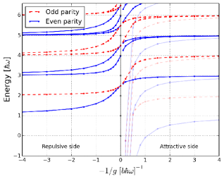
Figure 1: Three-body spectral flow. The energy spectrum of two $A$ and one $B$ particle as a function of interaction strength, $g$, obtained by numerical calculations. In the limit $1/g\to 0$, the ground state becomes doubly degenerate and has half-integer energy. The contribution from center-of-mass motion has been removed. For visibility, we have removed states from the attractive side that diverge to large negative energies close to $1/g\to 0$.

II Energetics and wave functions

Our two-component bosonic system has $N=N_{A}+N_{B}$ particles split between $N_{A}$ and $N_{B}$ identical bosons of two different kinds. All $N$ particles have mass $m$ and move in the same external harmonic trapping potential with single-particle Hamiltonian $h_{0}=\frac{p^{2}}{2m}+\frac{1}{2}m\omega^{2}x^{2}$, where $p$ and $x$ denote the momentum and position of either an $A$ or $B$ particle and $\omega$ is the common trap frequency. The trap provides a natural set of units for length, $b=\sqrt{\hbar/m\omega}$, and energy, $\hbar\omega$, which we will use throughout (here $\hbar$ is Planck’s constant divided by $2\pi$). We assume short-range interactions between $A$ and $B$ particles that we model by a Dirac delta-function parameterized by an interaction strength, $g$, i.e.

$$H_{I}=g\sum_{i=1}^{N_{A}}\sum_{j=1}^{N_{B}}\delta(x_{i}-y_{j}),$$ (1)

where $x$ and $y$ denote the coordinates of $A$ and $B$ particles, respectively. The intraspecies interaction strengths are assumed to be much smaller than $g$ and we will therefore neglect such terms. To access the quantum mechanical properties of our system we must solve the $N$-body Schrödinger equation. This will be done using novel analytical tools and using exact diagonalization. In the latter case we have adapted an effective interaction approach that has recently been succesfully applied to fermions in harmonic traps rotureau2013 ; lindgren2014 (see the Methods section for further details). The analytical and numerical methods allow us to address up to ten particles, which is larger than most previous studies not based on stochastic or Monte Carlo techniques.

The simplest non-trivial case is the three-body system which has two $A$ and one $B$ particle. The energy spectrum is shown in Fig. 1 as a function of $g$. The most interesting feature to notice is the ground state behaviour as $1/g\to 0^{+}$. Here, an odd and an even state become degenerate at an energy of $2.5\hbar\omega$. This should be contrasted to the behaviour of single-component bosons or two-component fermions which will always have energies that are an integer times $\hbar\omega$ when $1/g\to 0$. Furthermore, we notice how the two states that merge at $1/g=0$ become two excited state branches on the attractive side of the resonance but the even parity state remains the lower one. This is opposite to the behaviour of fermions volosniev2013 where the hierarchy of states is inverted at $1/g=0$. The ground state for large and negative $g$ is very different as it contains deeply bound molecules, which we will not consider further. The fractional energies in the spectrum can be explained by a schematic three-body model and in stochastic variational calculations zinner2013 . This provides a hint that larger systems could also display fractional energy states in the strongly interacting limit and begs the question as to what spatial configurations such states correspond to.

We will now show that the fractional energy states are generic for strongly interacting two-component bosons in 1D and, importantly, for the ground state they realize perfect ferromagnetic behaviour irrespective of whether the system is balanced ($N_{A}=N_{B}$) or not. The term perfect ferromagnetic behaviour implies that we have a full spatial separation of the two components in the exact ground state wave function of the system, i.e. the probability to find only $A$ on one side and only $B$ on the other side of the system is not just dominant, it is exactly unity. The ground state has only a single ’domain wall’ at which an $A$ and a $B$ particle are neighbours. As a consequence, imagine that you detect an $A$ particle on the left (right) side of the system, then you can immediately conclude that all the $B$ particles reside to the right (left) of this $A$ particle.

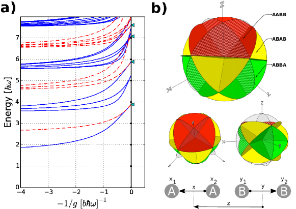
Figure 2: Balanced four-body system. a) Energy spectrum for $g>0$ for two $A$ and two $B$ particles. The $1/g\to 0^{+}$ limits are analytically known and indicated by triangles. Even parity states are in blue while odd parity states are red. b) Three-dimensional representation of the coordinate space on which the four-body wave function is defined when the center-of-mass position is removed. The specific Jacobi coordinates used are shown at the bottom. The solid coloured circular planes indicate the planes where an $AB$ pair overlap. The wave function must vanish on these planes in the limit where $1/g\to 0$. The checkerboard coloured circular planes are reflection planes for a pair of identical particles ($x\to-x$ and $y\to-y$). The red region has twice the volume of the green region and four times that of the yellow region. The smaller figures in the middle show the same regions viewed from different angles for clarity.

II.1 Balanced systems

We first consider a four-body system that has two $A$ and two $B$ particles. The energy spectrum for $g>0$ is shown in Fig. 2a). A striking feature is the two-fold degenerate ground state for $1/g\to 0$ that has a non-integer energy similar to the three-body problem. In this strongly repulsive limit, the system realizes a perfect spatially ferromagnetic quantum state as we will now demonstrate analytically.

First we note that the center-of-mass motion of the four-body system can be separated and thus ignored. This leaves three Jacobi coordinates to describe the system. The details of these reductions can be found in the Methods section below. In Fig. 2b) we show the space of the Jacobi coordinates and highlight all the planes at which an $AB$ (solid planes), an $AA$ or a $BB$ (checkerboard planes) pair of particles overlap. The main observation is that as $1/g\to 0$, the wave function must vanish on all the solid planes in Fig. 2b) and we arrive at the disconnected regions shown with different colours. The particles become effectively impenetrable and we may characterize the wave function by specifying the amplitudes of all possible spatial configurations of the four particles. These regions correspond to specific orderings on a line of the four particles. In particular, the large (red) region dominating the figure corresponds to spatial configurations $AABB$ or $BBAA$. The green region occupies half the spatial volume of the red and corresponds to $ABBA$ or $BAAB$, while the yellow region has one-fourth the volume of the red region and corresponds to $ABAB$ or $BABA$ configurations. A wave function that vanishes on all $AB$ interfaces may now be constructed in each of these regions. However, it is immediately clear that it will have lower energy when it can spread over a larger volume. We thus conclude that the doubly degenerate ground state at $1/g\to 0$ has the structure $AABB\pm BBAA$ (taking into account the parity invariance of the Hamiltonian).

As discussed in the Methods section, one may solve a simple wave equation in the red region and obtain the ground state energy to arbitrary precision. The triangles at the $1/g=0$ line in Fig. 2a) show the energies obtained in this manner. We reproduce both the ground state and a set of excited states. All of these have fractional energies and all of them are perfectly ferromagnetically ordered. The remaning states of the spectrum can be obtained by solving in the other regions of Fig. 2b). Note that states with amplitude exclusively in the yellow regions are perfectly spatial antiferromagnetic, $ABAB\pm BABA$, and have energies $n+1/2$ $\hbar\omega$ with integer $n$. They are the only parts of the spectrum which can be constructed by starting from identical fermions using Girardeau’s mapping techniques girardeau1960 . The arguments presented here are neither restricted to $N=4$ nor to a harmonic trapping potential and hold for any $N$ and any shape of the external confinement. They hinge only on the fact that the $AABB$ or $BBAA$ configurations occupy the largest volume. For instance, for $AABB$ the four regions $x_{1}<x_{2}<y_{1}<y_{2}$, $x_{2}<x_{1}<y_{1}<y_{2}$, $x_{1}<x_{2}<y_{2}<y_{1}$ and $x_{2}<x_{1}<y_{2}<y_{1}$ are adjacent regions and are connected by Bose symmetry of each component, thus they make up the connected upper red region ($z>0$) of the coordinate space in Fig. 2b). For $ABBA$ one finds that only $x_{1}<y_{1}<y_{2}<x_{2}$ and $x_{1}<y_{2}<y_{1}<x_{2}$ are adjacent and connected. This implies that the volume for $ABBA$ is half as large.

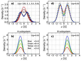
Figure 3: Ground state densities of balanced systems. a) Total density for $N_{A}=N_{B}=2$ and different values of $g$. Dotted (red) line corresponds to $1/g=100$ while the solid (black) line is for $1/g=0.01$. The dots show the analytical solution for $1/g=0$. b) and c) Densities for an equal superposition (sum) of the (nearly) two-fold degenerate ground state at $1/g=0.01$ for $N_{A}=N_{B}=2$, 3, 4, and 5. b) shows $A$ particles and c) shows $B$ particles. d) Rescaled plot of the total density at $1/g=0.01$. For $N_{A}=N_{B}<5$ the density has been rescaled to a total density with $N_{A}=N_{B}=5$. The dashed line corresponds to the density expected in the many-body limit $N_{A}=N_{B}\gg 1$.

Larger systems may in principle be handled in similar fashion by solving wave equations with proper boundary conditions and obtaining the fractional energies in the limit $1/g\to 0$. However, the increase in dimension of the problem makes this very difficult in practice. In order to further demonstrate that balanced systems have perfect ferromagnetic ground states irrespective of particle number, we have numerically computed the ground state densities for systems with $N_{A}=N_{B}\leq 5$ as shown in Fig. 3. Evidence of the separation of $A$ and $B$ can be seen in the total density already in Fig. 3a) for $N_{A}=N_{B}=2$ as $g$ increases (note the perfect agreement with the analytical result in the limit $1/g\to 0$). We expect the two degenerate ground states to have structure $A\ldots AB\ldots B\pm B\ldots BA\ldots A$. In order to prove this perfect ferromagnetic behaviour, we consider the odd and even superposition of the two degenerate states which we expect will yield states with exclusively $A$ or $B$ particles on either side of the system (corresponding to $A\ldots AB\ldots B$ or $B\ldots BA\ldots A$). The corresponding densities are shown in Fig. 3b) and Fig. 3c) and beautifully confirm our expectations.

As the ground state for $1/g\to 0$ is spatially separated, one may speculate that it can be understood physically as two ideal Bose gases or ’condensates’ sitting on either side of the system even in this strongly interacting limit. In Fig. 3d) we plot the densities in a rescaled fashion where we multiply by $5/2$, $5/3$, and $5/4$ on the $N_{A}=N_{B}=2$, $3$ and $4$ densities respectively. The convergence of the results toward the $N_{A}=N_{B}=5$ case indicates that the system does behave as two ideal Bose gases as the particle number grows. In the limit $N_{A}=N_{B}\gg 1$, we would expect the overlap of the two gases to vanish as the energy cost of overlap goes to infinity. We therefore expect that the occupied mode in this large system limit is the first excited state of the harmonic trap which vanishes at the center. The dashed line in Fig. 3d) shows this state rescaled to $N_{A}=N_{B}=5$. This analytical guess displays the same features as the numerical densities and we conclude that already for ten particles the many-body properties are emerging.

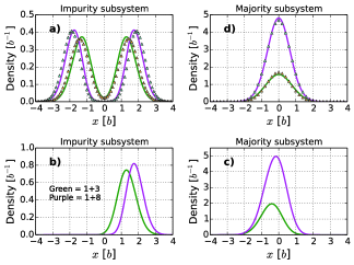
Figure 4: Ground state densities of imbalanced systems. a) Impurity density in an $N_{B}=3$ or $N_{B}=8$ system with $N_{A}=1$. The analytical results for $1/g=0$ are shown as triangles. b) and c) as in Fig. 3b) and c) but for $N_{A}=1$ with $N_{B}=3$ or $N_{B}=8$. d) The density of the majority component ($N_{B}$). All numerical results have been obtained with $1/g=0.01$.

II.2 Imbalanced systems

The extremely imbalanced limit, where $N_{A}=1$ and $N_{B}$ varies, provides a realization of a strongly interacting Bose polaron in 1D, i.e. an impurity that interacts strongly with an ideal Bose gas. In Fig. 4 we plot the densities of systems with $N_{A}=1$ and $N_{B}=3$ or $N_{B}=8$. We see that the impurity sits at the edge of the system (Fig. 4a)), while the majority component tends to occupy the center (Fig. 4d)). We confirm the numerical results by employing an analytical model, which shows excellent agreement. The details can be found in the Methods section. To confirm that the wave function of the strongly interacting ground state has intrinsic phase separation, i.e. has the form $AB\ldots B\pm B\ldots BA$, we plot the densities for a sum of the nearly degenerate ground states in Fig. 4b) and c). As in the balanced case above, we find a perfectly separated ground state behaviour. For instance, if we locate the single $A$ particle on one side of the trap, we would thus immediately know that all the $B$ particles reside on the other side, and vice versa. This behaviour is opposite to the case where the $B$ particles are identical fermions where the impurity resides mainly in the center of the system lindgren2014 . We have confirmed that this structure is also present for $N_{A}\neq N_{B}$ with $N_{A}>1$, and it is therefore a generic feature that the two species are perfectly spatially separated (ferromagnetic) in the ground state for strong interactions.

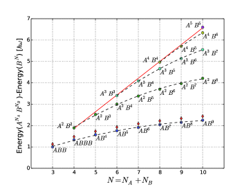
Figure 5: Ground state energies for $N\leq 10$. The filled circles show the ground state energy for $1/g=0.01$ relative to the zero-point energy as given by a single-component system of the same size. Each point is marked with the number of particles using the notation $A^{N_{A}}B^{N_{B}}$. The diamonds are the results of the analytical method for the polaron case described in the Methods section. The dashed lines are quadratic interpolations for fixed number of $B$ particles, while the solid line is an interpolation of the energy for the balanced systems.

A remarkable feature of the densities in Fig. 4b) and c) is the movement of the centroids of the peaks with particle number. We clearly see the majority moving into the center and the impurity being pushed toward the edge. This demonstrates how an ideal condensate is being built in the center. For large $N_{B}$ the energy per particle goes to $1/2\hbar\omega$, which implies a single-mode condensate that is becoming macroscopically occupied (see Methods section for details). The relative deviation between numerical and analytical energies is below three percent for $N_{B}\geq 9$. We thus have an analytic model for the crossover between the few- and many-body limit for the bosonic polaron in one dimension. This includes the external trap that is a reality of most experiments.

III Discussion

We have shown that a mixture of two ideal Bose systems in one dimension has unusual properties when the inter-species interactions is strong. The systems have energies that are non-integer multiples of $\hbar\omega$. In Fig. 5 we show the ground state energies for $1/g=0.01$ in systems with ten particles or less relative to a ground state with only $B$ particles. Driving an $A$ to $B$ transition via radiofrequency spectroscopy would be a possible way to confirm the predicted energies in Fig. 5. This technique has been demonstrated for fermions in recent few-body experiments in 1D wenz2013 . The results in Fig. 5 show that the energy per particle tends to saturate for large systems and that this happens faster the more imbalanced the system is. We also see that the balanced case has an almost linear energy dependence.

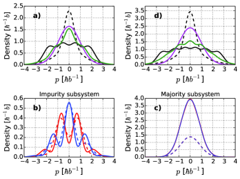
Figure 6: Momentum distributions. a) $N_{A}=N_{B}=2$ system. The even parity ground state is shown in purple, while the lowest excited state with antiferromagnetic structure is shown in green. For comparison the four-peak black curve represents identical fermions while the narrow peak dashed black curve shows hard-core bosons. b) Ground state impurity distributions for the even (blue) and odd (red) ground states with $N_{B}=8$ (solid) and $N_{B}=3$ (dashed). c) Ground state majority distributions for $N_{B}=8$ (solid) and $N_{B}=3$ (dashed). The even and odd parity results coincide for the majority. d) The same as in a) for $N_{A}=N_{B}=3$. All curves in the plot have been obtained for $1/g=0.01$.

The ferro- and antiferromagnetic states can also be detected by measuring momentum distributions. In Fig. 6a) and d) we show the distributions for $1/g=0.01$ with $N_{A}=N_{B}=2$ and $N_{A}=N_{B}=3$, respectively. The purple solid line is the even parity ground state while the solid green line is the excited state with antiferromagnetic ordering. The striking difference of the two distributions implies that they should be easily identifiable in experiments. For comparison, the solid black line with a multi-peak structure shows the distribution for a system of identical fermions. Comparing the solid green and black curves in Fig. 6a) and d) clearly demonstrates that, in spite of the fact that these two states have equal energy, the correlations are very different. In Fig. 6a) the dashed black line corresponds to the Tonks-Girardeau hard-core boson state girardeau1960 , which is also seen to be very different from the states discussed here. For imbalanced systems, we find that measuring the impurity momentum distribution, Fig. 6b), yields information about the parity of the state. On the other hand, the majority distributions in Fig. 6c) are identical in the two opposite parity ground states. A characteristic feature seen in Fig. 6b) is the development of oscillatory structure as the number of majority particles increases and pushes the impurity further out in the trap, see also Fig. 4b).

The separation of components in the ground state is intrinsic to both balanced and imbalanced mixtures, as is the presence of other spatial configurations in specific excited states. The effect is not connected to the harmonic confinement considered here and should be seen in an arbitrary confining geometry. A simple physical picture can be given in terms of domain walls, i.e. points at which the two components interface. The system tends to minimize the number of domain walls and this principle can be used to understand the ferromagnetic ground state and predict the ordering in energy of other configurations. In the paradigmatic two-component (spin 1/2) Fermi system, the ground state is never purely ferro- or antiferromagnetic for strong interactions volosniev2013 , and Bose mixtures therefore provide a unique set of quantum ground states for exploring and exploiting magnetic behaviour. The description of these systems clearly goes beyond the famous Bose-Fermi mappings girardeau1960 ; girar2004 and we provide not only numerical but also new analytical tools to fill this gap. Importantly, we demonstrate that the crossover from few- to many-body physics can be studied already at the level of ten particles.

IV Acknowledgements

This work was funded by the Danish Council for Independent Research DFF Natural Sciences and the DFF Sapere Aude program and the European Research Council under the European Community’s Seventh Framework Programme - ERC grant agreement no. 240603.

Appendix A Numerical method

We solve numerically the many-body Schrödinger equation by exact diagonalization with the full Hamiltonian projected onto a finite basis constructed from harmonic oscillator single-particle states. Each many-body basis state is written as a product of symmetrized states of $N_{A}$ and $N_{B}$ particles. The model space truncation is defined by an upper limit of the total energy.

Instead of the bare zero-range interaction in (1), we consider an effective two-body interaction in order to speed up the convergence of the eigenstates with respect to the size of the many-body basis. The effective potential is constructed in a truncated two-body space, and is designed such that its solutions correspond to exact two-body solutions given by the Busch formula busch1998 . As explained in detail in Refs. rotureau2013, ; lindgren2014, , this is achieved using a unitary transformation that involves the lowest eigensolutions given by the Busch formula. By construction, this unitary transformation approach will reproduce exact bare Hamiltonian results for the many-body system (both energy spectrum and wave functions) in the limit of infinite model space.

The excellent convergence property of this effective-interaction approach was demonstrated in Ref. lindgren2014 and is key to the quality of our numerical results and to our conclusions. In the construction of the effective interactions we benefit from having access to the exact two-body solutions for short-range interactions in harmonic traps. However, we stress that using numerical two-body solutions this approach can be generalized to study many-body systems in higher dimensions with finite-range interactions and in any trapping potential.

Appendix B Analytics for balanced systems

Here we outline the calculational procedures required to obtain the exact solutions for the $N_{A}=N_{B}=2$ four-body system in the $1/g\to 0$ limit. The method can in principle be extended to larger systems, but it becomes increasingly difficult. In the next subsection we provide an alternative method that works well for larger systems in the imbalanced case.

Denote the $A$ coordinates by $x_{1},x_{2}$ and the $B$ coordinates by $y_{1},y_{2}$, see Fig. 2b). The Hamiltonian is

$$H= \sum_{i=1}^{2}\left[\frac{p_{x_{i}}^{2}}{2m}+\frac{1}{2}m\omega^{2}x_{i}^{2}+\frac{p_{y_{i}}^{2}}{2m}+\frac{1}{2}m\omega^{2}y_{i}^{2}\right]$$

$$+g\delta(x_{1}-y_{1})+g\delta(x_{1}-y_{2})+g\delta(x_{2}-y_{1})+g\delta(x_{2}-y_{2}),$$ (2)

with $g$ the $AB$ interacting coupling constant and we assue that the $AA$ and $BB$ interactions vanish. We now perform an orthogonal coordinate transformation

$$\left[\begin{matrix}x\\ y\\ z\\ R\end{matrix}\right]=\left[\begin{matrix}\frac{1}{\sqrt{2}}&-\frac{1}{\sqrt{2}}&0&0\\ 0&0&-\frac{1}{\sqrt{2}}&\frac{1}{\sqrt{2}}\\ \frac{1}{2}&\frac{1}{2}&-\frac{1}{2}&-\frac{1}{2}\\ \frac{1}{2}&\frac{1}{2}&\frac{1}{2}&\frac{1}{2}\end{matrix}\right]\left[\begin{matrix}x_{1}\\ x_{2}\\ y_{1}\\ y_{2}\end{matrix}\right],$$ (3)

where $x,y,z$ are as shown at the bottom of in Fig. 2b) while $R$ denotes the center-of-mass coordinate. The quadratic kinetic and harmonic oscillator terms in $H$ retain their form under this transformation and one may immediately separate the center-of-mass, $R$, which can be ignored from now on. For the remaining three coordinates we switch to the usual spherical coordinate system, i.e. $\bm{r}=(x,y,z)$, $r=\sqrt{x^{2}+y^{2}+z^{2}}$, $\tan(\phi)=y/x$, and $\cos(\theta)=z/r$. Carrying out these transformation we arrive at the relative Hamiltonian

$$H_{\textrm{rel}}=-\frac{\hbar^{2}\bm{\nabla}^{2}}{2m}+\frac{1}{2}m\omega^{2}\bm{r}^{2}+\frac{g}{r}\sum\delta(\cos\theta\pm\sin\theta\sin(\pi/4\pm\phi)),$$ (4)

where the sum in the interaction term runs over the four combinations of signs in the argument of the delta function. The first two terms constitute a 3D harmonic oscillator with the well-known regular solution $\Psi(r,\theta,\phi)=N_{nl}r^{l}e^{-r^{2}/2b^{2}}L^{l+1/2}_{(n-l)/2}(r^{2}/b^{2})Y_{lm}(\theta,\phi)$, where $b=\sqrt{\hbar/m\omega}$ and $L_{a}^{b}(x)$ is the generalized Laguerre polynomial.

When $g=0$, the angular functions, $Y_{lm}(\theta,\phi)$, are the usual spherical harmonic functions with $l$ the total and $m$ the projection angular momentum quantum number. However, in the limit $1/g\to 0$ we have to enforce non-trivial boundary conditions whenever $A$ and $B$ particles overlap. Let us focus on the region $z>0$ by restricting to $0\leq\theta\leq\pi/2$ (solutions for $z<0$ may be obtained by symmetry arguments or by considering instead $\pi/2\leq\theta\leq\pi$). The arguments of the Dirac delta-functions in Eq. (4) vanish when

$$1\pm\tan\theta\sin(\pi/4\pm\phi)=0.$$ (5)

If we define $\tilde{\phi}=\phi+\pi/4$, we have $1\pm\tan\theta\sin\tilde{\phi}=0$ and $1\pm\tan\theta\cos\tilde{\phi}=0$. The regions defined by these conditions are illustrated in Fig. 2b). The solid red planes show exactly where the arguments of the interaction Dirac delta-functions have to vanish.

We now make the simple transformation $u=\tan\theta\sin\tilde{\phi}$ and $v=\tan\theta\cos\tilde{\phi}$. In these new $u,v$ variables, the boundaries are simply $1\pm u=0$ and $1\pm v=0$, i.e. the function must vanish on the boundary of a square. Finally, one must transform the angular part of the Laplacian into the new variables which yields

$$\nabla_{\theta,\phi}\to\nabla_{u,v}=\left(1+u^{2}+v^{2}\right)\times$$

$$\left((1+u^{2})\frac{\partial^{2}}{\partial u^{2}}+(1+v^{2})\frac{\partial^{2}}{\partial v^{2}}+2uv\frac{\partial^{2}}{\partial u\partial v}+2u\frac{\partial}{\partial u}+2v\frac{\partial}{\partial v}\right).$$ (6)

By the procedure outlined above we have transformed the problem of solving a harmonic oscillator problem in a non-trivial geometry, i.e. the red region in Fig. 2b), into solving a very simple boundary value problem

$$\nabla_{u,v}f(u,v)=\lambda(\lambda+1)f(u,v)$$ (7)

with $f(u,v)=0$ for $u,v=\pm 1$. We write the eigenvalue in this way so it matches the usual 3D angular eigenvalue $l(l+1)$. The equation for $f(u,v)$ may be straighforwardly solved by using a two-dimensional Fourier expansion of the wave function. This will produce some spurious solutions as we must also impose bosonic symmetry among the two $A$ and two $B$ particles separately. This translates to the requirement that the solution be symmetric when reflected across the two diagonals. Notice that for each eigenvalue of this problem, $\lambda$, we obtain a whole class of solutions with energies $E/\hbar\omega=2n+\lambda+3/2$ as we may add radial excitations.

The low-lying solutions of Eq. (7) are given in Tab. 1. State number 1, 4, 6, 11, 13, and 15 have the required bosonic symmetries for the balanced system. A number of doubly degenerate states in the spectrum may be used to construct eigenfunctions for a four-body system with $N_{A}=3$ and $N_{B}=1$ (or vice versa). In this case the wave function must vanish on the diagonal of the $(u,v)$ square domain which is achievable by taking proper linear combinations. The states marked ’fermions’ in Tab. 1 are antisymmetric across the two diagonals in the $(u,v)$ square and provide allowed states for all four-body two-component Fermi systems, i.e. 2+2, 3+1 or four identical fermions. The eigenenergies of the fermionic states have the exact values 7.5, 10.5 and 11.5. Our results differ by $4\cdot 10^{-5}$ which attests to the accuracy of our method. All states in Tab. 1 have been obtained using a modest 400 Fourier basis states. Notice that even though the lowest perfectly antiferromagnetic state for $N_{A}=N_{B}=2$ bosons is at the same energy as the fermionic state number 5 in Tab. 1, they are not related since states with the configurations $ABAB$ or $BABA$ solve a different boundary value problem (corresponding to the yellow regions in Fig. 2b)).

State	$\lambda+1.5$	System
1	3.88989	2+2 bosons
2	5.64323	3+1 bosons
3	5.64323	3+1 bosons
4	7.07740	2+2 bosons
5	7.50002	fermions
6	7.60232	2+2 bosons
7	8.76318	3+1 bosons
8	8.76318	3+1 bosons
9	9.52342	3+1 bosons
10	9.52342	3+1 bosons
11	10.21574	2+2 bosons
12	10.50004	fermions
13	10.73383	2+2 bosons
14	11.50004	fermions
15	11.51706	2+2 bosons
16	11.85409	3+1 bosons
17	11.85409	3+1 bosons

Table 1: Low-lying spectrum of Eq. (7). The last column denotes the specific system for which the particular solution is an allowed eigenstate using the notation $N_{A}+N_{B}$ for bosons. See the text for details.

The energies obtained using this (semi)-analytical approach for the $N_{A}=N_{B}=2$ system are given in Fig. 2a) as triangles at $1/g=0$. The two lowest triangles correspond to the angular ground state (lowest $\lambda$ value) with $n=0$ and $n=1$. The two upper triangles are the first and second excited angular solutions both with $n=0$. All four solutions have the spatial structure $AABB\pm BBAA$. The blue dots in Fig. 3a) show the ground state density obtained by the transformation method discussed here. The rest of the spectrum at $1/g\to 0$ can be obtained by solving the boundary value problem in the green ($ABBA\pm BAAB$) and yellow areas ($ABAB\pm BABA$). In the latter case a fermionized (totally antisymmetric) wave function is a solution. Our main interest here is to understand the ground state so we leave the remaining states and regions for future investigations.

Appendix C Analytics for imbalanced systems

The analytics provided here is applied for the Bose polaron, $N_{A}=1$ and $N_{B}$ arbitrary, but can be extended to other systems. The Hamiltonian can be written

$$H=h_{0}(x_{1})+\sum_{i=1}^{N_{B}}h_{0}(y_{i})+g\sum_{i=1}^{N_{B}}\delta(x_{1}-y_{i}),$$ (8)

where $h_{0}(z)=p_{z}^{2}/2m+m\omega^{2}z^{2}/2$ is a 1D harmonic oscillator. The $x_{1}$ coordinate denotes the single $A$ particle, the ’impurity’, while $y_{i}$ denotes the coordinates of the majority $B$ particles. We introduce an adiabatic decomposition of the total wave function of the form

$$\Psi(x_{1},y_{1},\ldots,y_{N_{B}})=\sum_{j}\phi_{j}(x_{1})\Phi_{j}(y_{1},\ldots,y_{N_{B}}|x_{1}),$$ (9)

where $\Phi_{j}$ is a normalized eigenstate of the eigenproblem $\sum_{i=1}^{N_{B}}h_{0}(y_{i})\Phi_{j}=E_{j}(x_{1})\Phi_{j}$ which depends parametrically on $x_{1}$. This expansion can be related to the Born-Oppenheimer approximation in which case one may consider $x_{1}$ the ’slow’ variable (typically the nuclear coordinate in molecular physics). In the limit of interest $1/g\to 0$, we impose the condition that the total wave function vanishes for $y_{i}=x_{1}$, $i=1,\ldots,N_{B}$. This implies that $\Phi_{j}=0$ whenever $y_{i}=x_{1}$. Since there are no intra-species interactions among the $B$ particles, we can write

$$\Phi_{j}(y_{1},\ldots,y_{N_{B}}|x_{1})=S\prod_{i=1}^{N_{B}}f_{k_{i}}(y_{i}|x_{1}),$$ (10)

where $S$ denotes the symmetrization operator and $f_{k_{i}}(y_{i}|x_{1})$ is the $k$th normalized eigenstate of $h_{0}(y_{i})$ which satisfies the condition $f_{k_{i}}(y_{i}=x_{1})=0$. The index $j$ on $\Phi_{j}$ denotes the many different ways to distribute the $N_{B}$ particles among the eigenstates of $h_{0}(y_{i})$ with the appropriate boundary condition. The Schrödinger equation for $\phi_{j}(x_{1})$ can now be written

$$\left[h_{0}(x_{1})+E_{i}(x_{1})\right]\phi_{i}=\sum_{j}\left(Q_{ij}(x_{1})\phi_{j}+P_{ij}(x_{1})\frac{\partial\phi_{j}}{\partial x_{1}}\right),$$ (11)

where

$$P_{ij}(x_{1})=\langle\Phi_{i}|\frac{\partial}{\partial x_{1}}|\Phi_{j}\rangle_{y}$$ (12)

$$Q_{ij}(x_{1})=\frac{1}{2}\langle\Phi_{i}|\frac{\partial^{2}}{\partial x_{1}^{2}}|\Phi_{j}\rangle_{y}.$$ (13)

The subscript $y$ on the brackets denote integration over all $y_{1},\ldots,y_{N_{B}}$. Note that $P_{ii}=0$ and $Q_{ii}<0$ nielsen2001 .

As we are interested in the ground state, we assume that all the $B$ particles are in the same state, $f_{0}(y_{i}|x_{1})$, that we specify below. Since the nearest excited states are obtained by promoting one of the $B$ particles into a single-particle excited orbital, one can show that $P_{ij}$ and $Q_{ij}$ scales with $\sqrt{N_{B}}$ while $Q_{ii}$ scales with $N_{B}$. For large $N_{B}$ we can thus neglect all but the $Q_{ii}$ terms. Furthermore, in the ground state we expect to find all the $B$ particles on one side of the impurity. If we assume that all $B$ particles are to the left of the impurity, we can write the single-particle wave function, $f_{0}(x|z)$ for $x\leq z$, as

$$f_{0}(x|z)=A(z)e^{-x^{2}/2}U(1/4-\epsilon(z)/2,1/2,x^{2}),$$ (14)

for $z<0$ or $z\geq 0$ and $x\leq 0$, while for $z\geq 0$ and $x>0$ we write

$$f_{0}(x|z)=-A(z)e^{-x^{2}/2}U(1/4-\epsilon(z)/2,1/2,x^{2})$$

$$+2A(z)e^{-x^{2}/2}\frac{U(1/4-\epsilon(z)/2,1/2,0)}{M(1/4-\epsilon(z)/2,1/2,0)}M(1/4-\epsilon(z)/2,1/2,x^{2}).$$ (15)

Here $A(z)$ is a normalization factor, $U$ and $M$ are the Tricomi and Kummer confluent hypergeometric functions, and we have used $b=\sqrt{\hbar/m\omega}$ as the unit of length. Here $\epsilon(z)$ is a function that is chosen to satisfy the requirement $f(x=z)=0$. This is equivalent to finding the ground state solution of $h_{0}(x)$ for $x\leq z$ with the condition that the wave function must vanish at $z$.

Once we have determined the functions $f(x|z)$ and $\epsilon(z)$, we can compute the adiabatic potential for the ground state. We have

$$Q_{11}(x_{1})=-\frac{1}{2}N_{B}\langle\left(\frac{\partial f(y|x_{1})}{\partial x_{1}}\right)^{2}\rangle_{y}.$$ (16)

Furthermore, $E_{1}(x_{1})=N_{B}\epsilon(x_{1})$ by additivity. The Schrödinger equation for $\phi(x_{1})$ is then

$$\left(h_{0}(x_{1})+N_{B}\epsilon(x_{1})+N_{B}\langle\left(\frac{\partial f(y|x_{1})}{\partial x_{1}}\right)^{2}\rangle_{y}\right)\phi(x_{1})=E_{0}\phi(x_{1}).$$ (17)

The energy $E_{0}$ provides a variational upper bound to the exact energy.

The energies computed via this method for the polaron are shown in Fig. 5 and agree with the numerical results to within a few percent for the largest particle numbers in the figure. We expect the agreement to become better for even larger particle numbers. Furthermore, since we obtain the full wave function in an analytical form we may also compute the densities of both impurity and majority components. In Fig. 4a) we show the impurity densities for $N_{B}=3$ and $N_{B}=8$, while Fig. 4d) shows the corresponding majority density. We see a striking agreement between the numerical results and the analytically tractable model presented here. The model presented here can be extended to excited states and also to systems with $N_{A}>1$.

References

- (1) H. A. Bethe, Z. Physik 71, 205-226 (1931).
- (2) E. H. Lieb and W. Liniger, Phys. Rev. 130, 1605-1616 (1963).
- (3) J. B. McGuire, J. Math. Phys. 6, 432-439 (1965); ibid. 7, 123-132 (1966).
- (4) C. N. Yang, Phys. Rev. Lett. 19, 1312-1315 (1967).
- (5) E. H. Lieb and F. Y. Wu, Phys. Rev. Lett. 20, 1445-1448 (1968).
- (6) F. D. M. Haldane, Phys. Rev. Lett. 47, 1840 (1981).
- (7) F. D. M. Haldane, J. Phys. C: Solid State Phys. 14, 2585 (1981).
- (8) T. Giamarchi, Quantum Physics in One Dimension, (Oxford University Press Inc., New York, 2003).
- (9) M. A. Cazalilla, R. Citro, T. Giamarchi, E. Orignac and M. Rigol, Rev. Mod. Phys. 83, 1405 (2011).
- (10) B. Paredes et al., Nature 429, 277-281 (2004).
- (11) T. Kinoshita, T. Wenger, and D. S. Weiss, Science 305, 1125-1128 (2004).
- (12) T. Kinoshita, T. Wenger, and D. S. Weiss, Nature 440, 900-903 (2006).
- (13) E. Haller et al.,bScience 325, 1224-1227 (2009).
- (14) F. Serwane et al., Science 332, 336-338 (2011).
- (15) G. Zürn et al., Phys. Rev. Lett. 108, 075303 (2012).
- (16) A. N. Wenz et al., Science 342, 457 (2013).
- (17) G. Pagano et al., Nature Phys. 10, 198-201 (2014).
- (18) A. Recati, P. O. Fedichev, W. Zwerger, and P. Zoller, Phys. Rev. Lett. 90, 020401 (2003).
- (19) A. B. Kuklov and B. V. Svistunov, Phys. Rev. Lett. 90, 100401 (2003).
- (20) L.-M. Duan, E. Demler, and M. D. Lukin, Phys. Rev. Lett. 91, 090402 (2003).
- (21) E. Eisenberg and E. H. Lieb, Phys. Rev. Lett. 89, 220403 (2002).
- (22) B. Nachtergaele and S. Shannon, Phys. Rev. Lett. 94, 057206 (2005).
- (23) S. Zöllner, H. D. Meyer, and P. Schmelcher, Phys. Rev. A 78, 013629 (2008).
- (24) Y. Hao and S. Chen, Phys. Rev. A 80, 043608 (2009).
- (25) M. A. Garcia-March and Th. Busch, Phys. Rev. A 87, 063633 (2013).
- (26) M. A. Garcia-March et al., Phys. Rev. A 88, 063604 (2013).
- (27) M. A. Garcia-March et al., arXiv:1405.7595 (2014).
- (28) N. T. Zinner et al., arXiv:1309.7219 (2013).
- (29) B. Sutherland, Phys. Rev. Lett. 20, 98 (1968).
- (30) Y.-Q. Li, S.-J. Gu, Z.-J. Ying, and U. Eckern, Europhys. Lett. 61, 368 (2003).
- (31) J. N. Fuchs, D. M. Gangardt, T. Keilmann, and G. V. Shlyapnikov, Phys. Rev. Lett. 95, 150402 (2005).
- (32) X. Guan, M. T. Batchelor, and M. Takahashi, Phys. Rev. A 76, 043617 (2007).
- (33) B. I. Halperin and P. C. Hohenberg, Phys. Rev. 188, 898 (1969).
- (34) B. I. Halperin, Phys. Rev. B 11, 178 (1975).
- (35) M. B. Zvonarev, V. V. Cheianov, and T. Giamarchi, Phys. Rev. Lett. 99, 240404 (2007).
- (36) S. Akhanjee and Y. Tserkovnyak, Phys. Rev. B 76, 140408 (2007).
- (37) A. Matveev and A. Furusaki, Phys. Rev. Lett. 101, 170403 (2008).
- (38) A. Kamenev and L. Glazman, Phys. Rev. A 80, 011603(R) (2009).
- (39) J. Caux, A. Klauser, and J. van den Brink, Phys. Rev. A 80, 061605 (2009).
- (40) E. J. Lindgren, J. Rotureau, C. Forssén, C., A. G. Volosniev, and N. T. Zinner, New J. Phys. 16, 063003 (2014).
- (41) J. Rotureau, Eur. Phys. J. D 67, 153 (2013).
- (42) A. G. Volosniev, D. V. Fedorov, A. S. Jensen, M. Valiente, and N. T. Zinner, arXiv:1306.4610 (2013).
- (43) M. D. Girardeau, J. Math. Phys. 1, 516-523 (1960).
- (44) M. D. Girardeau and M. Olshanii, Phys. Rev. A 70, 023608 (2004).
- (45) T. Busch, B.-G. Englert, K. Rza̧żewski, and M. Wilkens, Found. Phys. 28, 549-559 (1998).
- (46) E. Nielsen, D. V. Fedorov, A. S. Jensen, and E. Garrido, Phys. Rep. 347, 373-459 (2001).