Evidence for Bolgiano-Obukhov scaling in rotating stratified turbulence using
high-resolution direct numerical simulations

Abstract

We report results on rotating stratified turbulence in the absence of forcing, with large-scale isotropic initial conditions, using direct numerical simulations computed on grids of up to $4096^{3}$ points. The Reynolds and Froude numbers are respectively equal to $Re=5.4\times 10^{4}$ and $Fr=0.0242$. The ratio of the Brunt-Väisälä to the inertial wave frequency, $N/f$, is taken to be equal to 4.95, a choice appropriate to model the dynamics of the southern abyssal ocean at mid latitudes. This gives a global buoyancy Reynolds number $R_{B}=ReFr^{2}=32$, a value sufficient for some isotropy to be recovered in the small scales beyond the Ozmidov scale, but still moderate enough that the intermediate scales where waves are prevalent are well resolved. We concentrate on the large-scale dynamics, for which we find a spectrum compatible with the Bolgiano-Obukhov scaling, and confirm that the Froude number based on a typical vertical length scale is of order unity, with strong gradients in the vertical. Two characteristic scales emerge from this computation, and are identified from sharp variations in the spectral distribution of either total energy or helicity. A spectral break is also observed at a scale at which the partition of energy between the kinetic and potential modes changes abruptly, and beyond which a Kolmogorov-like spectrum recovers. Large slanted layers are ubiquitous in the flow in the velocity and temperature fields, with local overturning events indicated by small Richardson numbers, and a small large-scale enhancement of energy directly attributable to the effect of rotation is also observed.

I Introduction

Rotating stratified flows are particularly important in the understanding of the dynamics of our planet and the Sun. Several of the key concepts needed in order to progress in predictions of the weather and in the global evolution of the climate depend crucially on a fundamental understanding of these flows. At different scales, different physical regimes become salient, and yet all scales interact. The nonlinear advection produces steepening, albeit slowly in the presence of strong waves. Thus, these fronts and turbulent eddies lead to enhanced dissipation and dispersion of particles and tracers, affecting the global energetic behavior of the atmosphere and climate systems, for example for atmospheric synoptic scales, and for oceanic currents, in the latter case modifying the meridional circulation. In the atmosphere, such effects on energetics can in turn impair assessments of whether a given super-cell can spawn a tornado, and they affect both the evaluation of hurricane intensity and of climate variability. Rotating stratified turbulence (RST hereafter) thus plays a crucial role in the dynamics of the atmosphere and oceans, with nonlinear interactions–responsible for the complexity of turbulent flows–having to compete with the waves due to rotation and stratification.

All of this takes place in the presence of a variety of other phenomena, including reactive chemical transport, biological or hydrological processes, as well as large-scale shear and bounday layers for example. One common approach is to tackle the problem in its entirety and construct a succession of models with increasing degrees of complexity. Conversely, one can take the simplest problem with what may be the most essential ingredients and examine the dynamics of such flows from a fundamental point of view, an approach taken in this paper. One of the inherent difficulties is the fact that such flows are represented, in the dry Boussinesq framework, by four independent dimensionless parameters, the Reynolds, Froude, Rossby and Prandtl numbers defined as:

$$Re=\frac{U_{0}L_{0}}{\nu},\ Fr=\frac{U_{0}}{L_{0}N},\ Ro=\frac{U_{0}}{L_{0}f},\ Pr=\frac{\nu}{\kappa}\ ,$$ (1)

where $U_{0}$ and $L_{0}$ are, respectively, a characteristic velocity and length scale, $\nu$ and $\kappa$ are the kinematic viscosity and scalar diffusivity (taken to be equal, $Pr=1$), $N$ is the Brunt-Väisälä frequency, and finally $f=2\Omega$ with $\Omega$ the rotation frequency. Other dimensionless parameters, combinations or variants of these basic ones, are commonly defined as well (see §II.3).

A number of studies have shown, at least in the absence of rotation, that the buoyancy Reynolds number $R_{B}=ReFr^{2}$ needs to be large enough for vigorous turbulence to develop in the small scales (see for example the review in [1] and references therein). Indeed, at $R_{B}=1$, the Ozmidov scale

$$\ell_{OZ}=2\pi\sqrt{\varepsilon_{V}/N^{3}},$$ (2)

at which isotropy recovers in a purely stratified flow, is comparable to the dissipation (or Kolmogorov) scale, $\ell_{\eta}=2\pi(\nu^{3}/\varepsilon_{V})^{1/4}$, where $\varepsilon_{V}=|dE_{V}/dt|$ is the rate of dissipation of kinetic energy (note these length scales are written for a domain with dimensionless length of $2\pi$, such that $k=2\pi/\ell$ is the wavenumber). For $R_{B}>>1$, a Kolmogorov range, typical of isotropic and homogeneous turbulence, develops before dissipation can become effective. One can similarly define the Zeman scale, $\ell_{\Omega}=2\pi\sqrt{\varepsilon_{V}/f^{3}}$, for recovery of isotropy in a purely rotating flow, as shown in [2].

According to the relative values of these parameters, several ranges can co-exist, with one effect overcoming others in each range (say, nonlinearities over wave motions or vice-versa). Thus, such flows support multi-scale interactions that have to be explicitly resolved. The interaction between oscillatory waves and steepening nonlinear interactions can also result, e.g., in the development of strong and localized vertical velocity fields [3]. Different spectra are also observed in the purely stratified case; for example, a spectrum shallower than $k^{-1}$ is obtained in [4], whereas spectra steeper than $k^{-3}$ are observed in several other studies (see [5] for a recent review of oceanic observations and analytical models). In both cases, non-local interactions between widely separated scales may well be dominant [6]. Thus, large scale separations have to be achieved in order to be able to unravel the different competing phenomena.

A high-resolution direct numerical simulation (DNS) of homogeneous isotropic turbulence on a grid of $4096^{3}$ points, with Taylor Reynolds numbers of up to 1200 was performed a decade ago [7, 8] (for the case of passive tracers and Lagrangian particles, see [9, 10]). For purely stratified flows, runs with a slightly smaller resolution were presented recently in [11], with grids up to $4096^{2}\times 2048$ points at the largest buoyancy Reynolds number, and $4096^{2}\times 512$ for the more strongly stratified flow. In these simulations, energy cascades are found both in the vertical and the horizontal directions, with 1/3 of the dissipation coming from the former as in three-dimensional (3D) homogenous isotropic turbulence, and with a Kolmogorov spectrum in terms of the horizontal wavenumber at scales both larger and smaller than the Ozmidov scale. Other DNSs of purely stratified flows at linear resolutions of up to 2048 points, at least in one direction, focus on the influence on the resulting dynamics and energy distribution among scales of resolving or not either the buoyancy scale characteristic of the thickness of the vertical layers

$$L_{B}=2\pi U_{0}/N\ ,$$ (3)

or the Ozmidov scale $\ell_{OZ}$ at which isotropy recovers [12, 13, 14]. Part of the difficulty in determining spectral distribution among scales resides in the well-known fact [15] that the dynamics is anisotropic, and thus the isotropic spectrum should be replaced by an axisymmetric two-dimensional spectrum, or by anisotropic correlation functions. Similar characteristic length scales can be defined on the rotation rate $f$, and in fact, when both rotation and stratification are present, other scales can be defined (see equations (16), (18)).

It should be noted that numerical simulations are quite complementary to laboratory experiments. In the latter case, the Reynolds number can be quite high, reaching in some cases geophysical values of $10^{5}$ or $10^{6}$, although Froude numbers often remain close to (but less than) unity [16, 17]. This means that the buoyancy Reynolds numbers $R_{B}$ are high as well in these cases, although the stratification is not so strongly felt. By contrast, DNSs can only be performed at still modest values of Reynolds numbers (up to $\approx 10^{4}$, unless some parametrization scheme for the unresolved small-scales is used), but the Froude numbers can be taken as low as $10^{-2}$ or even $10^{-3}$ (for laboratory flows at small buoyancy Reynolds number, see the recent review in [18]).

Figure 1: Temporal variations of (a) kinetic energy dissipation rate and (b) the ratio of kinetic to potential energy. In (a) is displayed with a dashed line (red) the run using the $3072^{3}$ grid which evolved until $t=6.7$. The green squares represent the run performed on the grid of $4096^{3}$ points, evolved for $5\leq t\leq 5.88$ (i.e., for a duration of $\approx 77$ gravity wave periods), and the black triangles indicate the early-time run on a grid of $1536^{3}$ points. All runs have the same physical parameters and time step.

While these results were obtained for purely stratified flows, the role of rotation on stratified turbulence has been investigated by a number of authors. Besides the energy, rotating stratified flows also conserve the pointwise potential vorticity which can be defined as $P_{V}=f\partial_{z}\rho-N\omega_{z}+\omega\cdot\nabla\rho$, with $\rho$ the density (or temperature) fluctuations, and $\omega=\nabla\times{\bf u}$ the vorticity, ${\bf u}$ being the velocity. Because of the nonlinear term $\omega\cdot\nabla\rho$ in the expression of $P_{V}$, its ${\cal L}_{2}$ norm is quartic and thus it is not conserved by each triadic interaction in a truncated ensemble of modes. The extent to which this is relevant to the dynamical evolution of the flow is not entirely known, but several studies for shallow water [19] or the Boussinesq equations [20, 21, 22] assess the relative importance of the different contributions to $P_{V}$, with the general assumption that the high-order terms can be neglected when the waves are strong enough, i.e., at small Froude and/or Rossby numbers. In contrast, for the particular case of stable stratification, it was hypothesized in [22] that when $R_{B}$ is large enough the nonlinear term in $P_{V}$ affects the dynamics, becoming important at the same time as Kelvin-Helmoltz instabilities develop in the flow.

Since in many cases of geophysical interest, the ratio of the stratification to rotation frequencies $N/f$ is quite high (of the order of 100), most studies of RST consider the case of weak rotation. In reduced models relevant for geophysical flows, the geostrophic balance that results (between pressure gradients, Coriolis force and gravity) and the quasi-geostrophic (QG) regime, are central tenets of large-scale behavior and have been studied extensively over the years [23, 24, 25, 26], including their breaking down through, for example, fronto-genesis [27].

Figure 2: Temporal evolution of (a) the ratio of the volume averaged vertical to horizontal kinetic energy, $\left<w^{2}\right>/\left<u^{2}+v^{2}\right>$, and (b) the vertical length scale $\ell_{z}$ defined in Eq. (13), which is characteristic of vertical shear layers. The integral scale $L_{int}$ is also provided in order to compare with $\ell_{z}$.

In the Boussinesq framework, a number of pioneering analyses of RST were performed in [28, 29, 30, 31, 32, 33, 34]. The role played by the ratio $N/f$ in these flows is relevant although, in some ways, poorly understood. In [28] it was shown that, while stratification in the absence of rotation determines the vertical length scale $L_{\parallel}$ (basically, the buoyancy scale $L_{B}$ associated with the thickness of vertical layers, with a Froude number based on this vertical length scale of order unity) independently of the horizontal scale, $L_{\perp}$, in RST this scale has a more complex dependence on the buoyancy scale and on $N/f$, in which Rossby number is the chief discriminating factor. However, specifically in the quasi-geostrophic limit, it is found [32] that $L_{\parallel}\propto fL_{\perp}/N$, with the proportionality indeed consisting of a function of Rossby number, as suggested in [28]. We use this finding to help explain spectral features in our DNS.

In [29], elongated boxes were considered to study the emergence of a direct energy cascade in RST with a Kolmogorov spectrum in the horizontal direction, and it was shown that such is the case provided the Rossby number is greater than a critical value of $\approx 0.1$. The case of large $N/f$ ($\gtrsim 45$) was also considered, and the runs were performed using hyper-viscosity. The aspect ratio of the computational domain seems to play an important role in these studies, and to influence the dynamics especially at unit Burger number $Bu=NL_{\perp}/fL_{\parallel}$. The linear regime of potential vorticity at $Bu=1$ was analyzed in [35] (see also [36]), and it was found that vortical modes dominate over waves at large scales, and that the parameter $\Gamma=fk_{\parallel}/(Nk_{\perp})$ is relevant as a measure of the relative importance of terms in the linear part of the expression for potential vorticity: the two sources of dispersion become comparable when $fk_{\parallel}\sim Nk_{\perp}$. A more recent work on RST [37] deals with the emergence of helicity (vorticity-velocity correlations) in such flows, helicity being measured to be relatively strong in tornadoes and hurricanes [38], and also being an important ingredient in the origin of large-scale magnetic fields in astrophysics.

Finally, besides DNS, rapid distortion theory for RST was considered in [33] where it was shown that $N/f$ governs the final distribution of energy among the horizontal and vertical kinetic energy components and potential modes, as well as the normalized vertical flux $\left<\rho w\right>$, where $w$ is the vertical velocity, together with the root mean square vertical vorticity, whereas stratification dominates the unsteadiness of these flows.

As already mentioned, $N/f$ is rather large in many applications. However, the case of RST with $N/f$ of order unity (or slightly larger) is also of interest for geophysical flows. One example is the abyssal southern ocean at mid latitude [39], which serves as a motivation for the present study and for which $N/f$ is estimated to be between roughly 5 and 10. Flows with $N/f$ ranging from $0.1$ to 10 were analyzed in [30, 31]; all runs were spin-down with initial conditions at $k_{0}\approx 10$. These authors stressed the importance of computing for long times compared to both the inertial and stratified periods of the waves, because of what are called slow modes, i.e., modes with zero wave frequency, as already emphasized in [34] (see also [40]. In [34], it was also noted that energy builds up with time at small scales, the flow being strongly intermittent. Previous studies in the regime of moderate $N/f$ also showed that the inverse cascade of energy to large scales is more efficient in the range $1/2\leq N/f\leq 2$ [41], when wave resonances disappear [34]. Moreover, when forcing RST at small scales, it can be shown that there is a clear tendency towards a $-5/3$ spectrum for the inverse cascade, as the Reynolds number increases for fixed parameters, together with the existence of a dual energy cascade: to small scales with a positive and constant energy flux, and to large scales with again a constant but negative energy flux [42].

Noticing the scarcity of high-resolution DNS for turbulence in the presence of both rotation and stratification to date, and considering the geophysical relevance of flows with moderate values of $N/f$, we thus now analyze results stemming from one such run with a numerical resolution using up to $4096^{3}$ grid points at the peak of dissipation. In the next section are given the equations, the numerical procedure and the overall parameters. Sections §III and §IV provide, respectively, the temporal and spectral dynamics of the flow, §V describes the physical structures that develop, and finally, §VI offers a brief discussion and our conclusions.

Figure 3: (a) High-resolution isotropic spectrum of the total energy, averaged over the time interval $t\in[5.3,5.7]$ corresponding to the peak in enstrophy, and compensated by a Kolmogorov 5/3 law. Note the break in the slope for $k\approx 12$. (b) Kinetic (solid line) and potential (dashed line) energy spectra compensated by $k^{11/5}$ and $k^{7/5}$, respectively, with the same temporal averaging. (c) Plot of total energy flux, and, separately, the kinetic and potential energy fluxes, as well as the buoyancy flux term obtained from Eq. (15). All fluxes are averated over the same time interval. Note the negative total flux at large scale, indicative of the effect of rotation. (d) Ratio of kinetic to potential energy spectra averaged over the same time interval; note again a transition around $k\approx 12$, and a scaling close to $k^{-4/5}$.

II Numerical set-up

II.1 Equations

The Boussinesq equations in the presence of solid body rotation, for a fluid with velocity ${\bf u}$, vertical velocity component $w$, and density (or temperature) fluctuations $\rho$, are:

$$\frac{\partial{\bf u}}{\partial t}+\mbox{\boldmath$\omega$}\times{\bf u}+2\mbox{\boldmath$\Omega$}\times{\bf u} = -N\rho\hat{e}_{z}-\nabla{\cal P}+\nu\nabla^{2}{\bf u}\ \ ,$$ (4)

$$\frac{\partial\rho}{\partial t}+{\bf u}\cdot\nabla\rho = Nw+\kappa\nabla^{2}\rho\ ,$$ (5)

together with $\nabla\cdot{\bf u}=0$ assuming incompressibility. ${\cal P}$ is the total pressure and $\hat{e}_{z}$ is the unit vector in the vertical direction which is in the direction of the imposed rotation and opposed to the imposed gravity; therefore, $\mbox{\boldmath$\Omega$}=\Omega\hat{z}$. The initial conditions for the velocity are centered on the large scales, with excited wavenumbers $k_{0}\in[2,3]$ and isotropic with random phases. In the absence of dissipation ($\nu=\eta=0$), the total energy $E_{T}=E_{V}+E_{P}$ is conserved, with $E_{V}=\frac{1}{2}\left<|{\bf u}|^{2}\right>$ and $E_{P}=\frac{1}{2}\left<\rho^{2}\right>$ respectively the kinetic and potential energies; the point-wise potential vorticity is also conserved. Lastly, $E_{P}=0$ initially.

Figure 4: Helicity dynamics using the data from the $4096^{3}$ run. (a) Relative helicity spectrum $|H_{V}(k)|/[kE_{V}(k)]$, which is seen as rather flat at large scale and decaying faster than $1/k$ at small scale. (b) Perpendicular spectrum of the helicity compensated with $k_{\perp}^{2}$. Note the region of excess helicity for small wavenumbers followed, for $k>k_{c}$ with $k_{c}\approx 12$, by a drop in the amplitude of the compensated spectrum, and with fluctuations associated with rapid changes in sign of the helicity. For $k>300$, a sharp drop is observed. (c) Temporal evolution of the volume integrated helicity. (d) Probability distribution function of the relative helicity (cosine of the angle between velocity and vorticity) at the peak of dissipation, $t=5.54$. Alignment and anti-alignment of ${\bf u}$ and $\omega$ are equally likely, as in homogeneous isotopic turbulence.

When linearizing the above equations in the absence of dissipation, one obtains inertia-gravity waves of frequency

$$\omega_{k}=k^{-1}\sqrt{N^{2}k_{\perp}^{2}+f^{2}k_{\parallel}^{2}}\,,$$ (6)

with $k=\sqrt{k_{\perp}^{2}+k_{\parallel}^{2}}$, $k_{\perp}=\sqrt{k_{x}^{2}+k_{y}^{2}}$, and $k_{\parallel}=k_{z}$, respectively the total, horizontal (or perpendicular), and vertical (or parallel) wavenumbers (see, e.g., [20, 43]). Fourier spectra will be built-up from their axisymmetric counterparts defined from the two-point one-time velocity covariance $U({\bf k})$ (see, e.g., [2])

$$e_{V}(|{\bf k}_{\perp}|,k_{\parallel})=\sum_{\begin{subarray}{c}k_{\perp}\leq|{\bf k}\times\hat{\bf z}|<k_{\perp}+1\\ k_{\parallel}\leq k_{z}<k_{\parallel}+1\end{subarray}}U({\bf k}) =\int U({\bf k})|{\bf k}|\sin\theta d\phi=e(|{\bf k}|,\theta)=e(k,\theta)\ ;$$ (7)

here $\phi$ is the longitude with respect to the $k_{x}$ axis and $\theta$ the co-latitude in Fourier space with respect to the vertical axis. The function $e_{V}({\bf k}_{\perp},k_{\parallel}=0)$ may be regarded as the spectrum of two-dimensional (2D) modes, having no vertical variation. Note that for an isotropic flow, at a given point ${\mathbf{k}}$ in wavenumber space, the ratio of the axisymmetric spectrum $e_{V}(|{\bf k}_{\perp}|,k_{\parallel})$ to the isotropic spectrum is $\sim 1/|{\bf k}|$ because the size of the volume element in the isotropic case contains an additional (integrating) factor of $|{\bf k}|$ compared to the axisymmetric case. Hence, if the axisymmetric spectrum behaves as $k_{\perp}^{-\alpha}$, then the corresponding isotropic scaling will be $k^{-\alpha+1}$. The spectrum $e_{V}(|{\bf k}_{\perp}|,k_{\parallel})$ can also be decomposed into the kinetic energy spectrum of the horizontal components (velocity components $u$ and $v$), and of the vertical kinetic energy (velocity component $w$):

$$e_{V}(|{\bf k}_{\perp}|,k_{\parallel})=e_{\perp}(|{\bf k}_{\perp}|,k_{\parallel})+e_{\parallel}(|{\bf k}_{\perp}|,k_{\parallel})\,.$$ (8)

In the following we will also consider the reduced perpendicular spectrum [44]

$$E_{V}(k_{\perp})=\Sigma_{k_{\parallel}}e_{V}({\bf k}_{\perp},k_{\parallel})\,,$$ (9)

the reduced parallel spectrum $E_{V}(k_{\parallel})$ (which has a sum over $k_{\perp}$), and the spectrum representing the perpendicular energy of the strictly three-dimensional (3D) modes:

$$E_{3D}(k_{\perp})=E_{V}(k_{\perp})-e_{V}({\bf k}_{\perp},k_{\parallel}=0)\,.$$ (10)

Similar definitions hold for the helicity and potential energy spectra, $h_{V}({\bf k}_{\perp},k_{\parallel})$ and $e_{P}({\bf k}_{\perp},k_{\parallel})$, their reduced forms, $H_{V}({\bf k}_{\perp})$ and $E_{P}({\bf k}_{\perp})$, as well as their 3D expressions (i.e., the perpendicular spectra of the 3D modes), $H_{V,3D}({\bf k}_{\perp})$ and $E_{P,3D}({\bf k}_{\perp})$. They will be analyzed in the following sections.

Figure 5: (a) Ratio $E_{3D}(k_{\perp})/e(k_{\perp},k_{\parallel}=0)$ of spectral energy in 3D modes versus that in 2D modes. Note again the transitions for $k\approx 12$ and $k\approx 300$. (b) Parallel spectrum of horizontal kinetic energy $e_{\perp}(k_{\perp}=0,k_{\parallel})$ (solid line, see equation (8)) and parallel spectrum of potential energy $e_{P}(k_{\perp}=0,k_{\parallel})$ (dashed line), both compensated by $k_{\parallel}^{-3}$. Power laws are indicated as references. All spectra are averaged over the peak of enstrophy, $t\in[5.3,5.7]$. Note the small flat range at large scales in $e_{\perp}$, both ending with equipartition at $k\approx 12$.

II.2 Specific numerical procedure

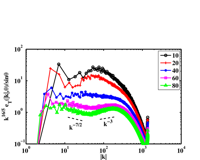
Figure 6: Angular total energy spectra $e(|k|,\theta)$ (Eq. (7)) for various co-latitude, $\theta$, (in degrees) averaged over the peak of enstrophy, $t\in[5.3,5.7]$, and compensated by $k(\theta)^{-16/5}$: $\theta=10^{\circ}$ (black circles), $\theta=20^{\circ}$ (red crosses), $\theta=40^{\circ}$ (blue asterisk), $\theta=60^{\circ}$ (magenta squares), and finally $\theta=80^{\circ}$ (green triangles). The compensating slope corresponds to an (uncompensated) isotropic (BO) scaling of $k^{-11/5}$.

Figure 7: Perspective volume renderings of a thin y-z sub-volume of size $0.4\times 0.7$ times the compute box size at $t=5.54$ (close to the peak of enstrophy). The y-axis is directed horizontally, and the z-axis, vertically. Presented are (a) perpendicular and (b) vertical velocity with identical color mapping. Note that the perpendicular velocity is dominant in magnitude. The slab thickness in the x (depth) direction is $0.04$ times the box size. All renderings were made using the using the VAPOR visualization system [47].

The code used in this paper is the Geophysical High Order Suite for Turbulence (GHOST), which is fully parallelized using a hybrid methodology [45]. It uses parallel multidimensional FFTs in a pseudo-spectral method for 2D and 3D domains on regular structured grid, and can solve a variety of neutral-fluid partial differential equations, as well as several that include a magnetic field. Boundary conditions are periodic, and the time-integration is performed using a Runge-Kutta algorithm up to 4th-order with double precision arithmetic. The code uses a “slab” (1D) domain decomposition among MPI tasks, and OpenMP threads provide a second level of parallelization within each slab or MPI task. The code demonstrates good parallelization to more than $100,000$ compute cores.

In order to achieve a high resolution at peak of dissipation when gradients of variables are the strongest, we have implemented a “bootstrapping” procedure in which we start the simulation at a lower resolution until the dynamic range of the energy spectrum decreases to some fiducial value. Here, by dynamic range we refer to the ratio of the energy at the peak of the spectrum, to the energy at the largest available wavenumber at a given resolution. When the lower threshold is reached, we increase the resolution and continue running until the dynamic range of the DNS at the new resolution decreases again to the fiducial value, repeating the process. Bootstrapping requires that a field at a reduced resolution be “padded” spectrally with zeros from its largest allowed wavenumber to the larger wavenumber allowed at the next (higher) resolution. This is handled in a processing step before the next highest resolution DNS is computed. This bootstrapping procedure was recently implemented, tested and used in the context of ideal magnetohydrodynamics [46].

We thus began with a $1536^{3}$ run up to $t=2$, then doubled the resolution on a grid of $3072^{3}$ grid points up to $t=5$, and then completed the run on the grid with $4096^{3}$ points. The maximum resolved wavenumber using a classical 2/3 de-aliasing rule is $k_{max}=N/3=1365$, with the length of the box corresponding to wavenumber $k_{min}=1$. The viscosity and scalar diffusivity were chosen to be the same for these three successive runs, each run representing the evolution of the same physical problem at earlier times. The time step for each was chosen on the basis of the highest resolution considered in order to minimize time stepping errors at lower resolution. The first bootstrapping was done during the inviscid phase before the small scale structures that can dissipate energy develop.

The run on the intermediate grid of $3072^{3}$ points, was also pursued to later times ($t_{max}=6.7$); this enabled us to inspect the convergence of the overall statistics at the same evolutionary times. Figure 1(a-b) displays the time evolution of the kinetic energy dissipation rate (proportional to the kinetic enstrophy $\left<|\omega|^{2}\right>$), and the ratio of the kinetic to potential energy, to illustrate the three distinct intervals with bootstraping and the overall evolution of the system.

II.3 Other dimensionless parameters

As mentioned in the introduction, a variety of dimensionless combinations of relevant physical parameters can be defined for rotating stratified turbulence, beyond those written in Eq. (1). One of the central limitations to a better understanding of such flows is the need to unravel what the key parameters are that govern the dynamics. Beyond the Reynolds, Froude, Rossby and Prandtl numbers, one also considers the ratio $N/f$, as well as the Froude number based on a characteristic vertical length scale,

$$F_{z}=U_{0}/(\ell_{Z}N)\ .$$

Moreover, the combined effect of turbulent eddies and waves can be encompassed in the buoyancy and rotational Reynolds numbers, mentioned previously and respectively defined as

$$R_{B}=ReFr^{2},\ R_{\Omega}=ReRo^{2}\ .$$ (11)

When $R_{B}\geq 1$ in a stratified flow, isotropy recovers beyond the so-called Ozmidov scale. Similarly, in a purely rotating flow, isotropy recovers beyond the Zeman scale for $R_{\Omega}\geq 1$ [2].

The partition of energy between kinetic and potential modes can be measured by their ratio, $E_{V}/E_{P}$, which is one possible definition of the Richardson number. Another definition is simply to measure the relative strength of the buoyancy to the inertial forces, or

$$Ri=1/Fr^{2}\ .$$

However, in order to emphasize the role of the development of small scales in mixing, one can also define a (local) Richardson number based on velocity gradients, $Ri_{g}$, as:

$$Ri_{g}=N(N-\partial_{z}\rho)/(\partial_{z}u_{\perp})^{2}\ .$$ (12)

This definition suggests that a sufficiently large vertical gradient locally leads to negative values of $Ri_{g}$, which is consistent with the intuitive picture of overturning when a denser parcel of fluid lies atop a less dense parcel.

II.4 Run parameters and general characterization

Figure 8: Perspective volume renderings of a thin x-z sub-volume of size $0.12\times 0.1$ times the compute box size at $t=5.54$ (close to the peak of dissipation); the slab thickness in the y-direction is 0.01 times the box size. The x-axis is directed horizontally, and the z-axis, vertically. Presented are (a) vorticity magnitude, (b) temperature fluctuations, and (c) local Richardson number $Ri_{g}$ defined in equation (12). The color bar of vorticity illustrates the relatively intense vortices that are generated, and note the slanted Kelvin-Helmoltz layer.

We use $N/f=4.95$ with $N=13.2$ and $\Omega=f/2=1.33$ (thus, $f=2.66$). The viscosity is chosen to have the simulation well resolved: $\nu=4\times 10^{-5}$. In dimensionless units, the resulting overall energetics of the flow lead to several scales that are of interest, and to a characterization of the flow in terms of the dimensionless parameters. Considered at the peak of enstrophy, the characteristic velocity is $U_{0}\approx 0.83$ and the integral length scale, computed from $L_{int}=2\pi\int E_{V}(k)dk/\int kE_{V}(k)dk\approx 2.6$, very close as expected to the scale at which the energy spectrum initially peaks, namely $L_{0}=2\pi/k_{0}\approx 2.5$. The dissipation rate of kinetic energy is taken from a computation of kinetic enstrophy at the peak of dissipation: $\varepsilon_{V}=\nu\left<|\omega|^{2}\right>\approx 0.0124$ (see Fig. 1(b)). Note that in the isotropic case, $\varepsilon_{V}=\epsilon_{K41}=U_{0}^{3}/L_{int}\approx 0.22$, but this relation does not hold in the highly anisotropic system we are investigating. Rather, we can take an estimate coming from weak turbulence, namely $\epsilon_{K41}*Fr\approx 0.005$, within a factor of two of the measured rate of energy dissipation. The Kolmogorov dissipation wavenumber is computed at the peak of dissipation to be $k_{\eta}\approx 660$. The Zeman and Ozmidov wavenumbers are therefore found to be, respectively, $k_{\Omega}\approx 39$ and $k_{OZ}\approx 431$. The buoyancy wavenumber is $k_{B}=2\pi/L_{B}\approx 16$; the lack of scale separation between $k_{\Omega}$ and $k_{B}$ suggests that it will be difficult to distinguish as separate effects those due to rotation and those due to stratification. The Reynolds number is thus found to be $Re\approx 5.4\times 10^{4}$, the Froude number $Fr\approx 0.0242$, and the Rossby number $Ro\approx 0.12$. Consequently, the buoyancy and rotational Reynolds numbers are $R_{B}\approx 32$, and $R_{\Omega}\approx 775$. The Richardson number is determined to be $Ri\approx 1700$, so the flow is, indeed, found to be strongly stratified.

Finally, we can define a Taylor Reynolds number as $R_{\lambda}=U_{0}\lambda/\nu$, with $\lambda=2\pi[\int E_{V}(k)dk/\int k^{2}E_{V}(k)dk]^{1/2}$ the Taylor scale. In classical homogeneous isotropic turbulence (HIT) $R_{\lambda}$ measures the degree of development of small scales. At peak of dissipation, $\lambda\approx 0.31$, leading to a rather large $R_{\lambda}\approx 6400$, quite high compared to similar computations in HIT (e.g., $R_{\lambda}\approx 1200$ in a HIT run at similar grid resolution [7, 8]). This is linked to the fact that, in the presence of strong waves, the transport of energy to small scales is hindered and not as efficient, and the energy spectrum becomes steeper at least at large scales, resulting in a larger Taylor scale for the same viscosity. It is worth noticing that in the atmosphere the Taylor Reynolds number is estimated to be $R_{\lambda}\approx 20000$, and it may be the case that realistic simulations of stratified and rotating atmospheric turbulence may be feasible in the near future as a result of this effect. Finally, note also that the value of $R_{\lambda}$ puts the present computation above the different thresholds in $R_{\lambda}$ identified in [48] for various instabilities to develop, as, e.g., for the growth of vertical shear and the growth of vertical energy.

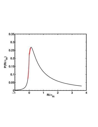
Figure 9: Probability distribution function of the gradient Richardson number defined in Eq. (12), at the latest time in the simulation. The (red) crosses indicate where $|Ri_{g}|\leq 0.25$, the classical criterion for overturning instability [49, 50].

When the dimensionless numbers obtained in the simulation at peak of dissipation given above are now dimensionalized using the characteristic length and velocity of the abyssal southern ocean at mid latitudes, i.e. with $L_{0}=1000$ m (corresponding to the peak of energy input in the ocean from bathymetry [51]) and $U_{0}=0.024$ m s^-1, as measured for example in the Drake passage [39], we obtain kinematic viscosity and scalar diffusivity, respectively, of $\nu=\kappa=4.5\times 10^{-4}$ m² s^-1, too large by roughly two orders of magnitude. The corresponding overall effective energy dissipation rate would be $\epsilon\sim U_{0}^{3}/L_{0}\approx 1.4\times 10^{-8}$ m² s^-3; this latter value corresponds to the enhanced dissipation measured in the southern ocean [52]. As a comparison, measurements in the atmosphere indicate $\epsilon\approx 10^{-6}$ m² s^-3 at intermediate altitude and at scales between 3 and $600$ km [53]. With a rotation frequency of $\Omega=10^{-4}\ s^{-1}$, our choice of parameters leads to a Brunt-Väisälä frequency of $N\approx 10^{-3}$ s^-1, and $Fr\approx 0.024$, corresponding to the parameters of the run described above. Then, the buoyancy scale is $150$ m, the Ozmidov scale is $4$ m, and the Kolmogorov dissipation scale is around $0.15$ m. This last value is too large, because the viscosity is too large and the numerical resolution is still insufficient. Also, note that another lacking element in our simulation is the interaction with a larger-scale (mean) flow, say at the scale of several hundred kilometers, together with proper boundary conditions in the vertical.

III Overall temporal dynamics

We now examine in more detail the overall temporal evolution of large-scale features. Figure 1(a-b) display, respectively, the kinetic energy dissipation, $\nu\left<\omega^{2}\right>$, and the ratio of kinetic to potential energy. Easily identifiable initial oscillations due to the waves prevail at early times; these oscillations, stronger and thus more visible at large scale in the evolution of the energy, are due to inertia-gravity waves and their irregularity is linked with nonlinear coupling which, at that Reynolds number, is sizable. However, the ratio of kinetic to potential energy remains relatively constant on average throughout the run after the initial phase, at a value close to 3. This initial phase is essential, since, even though our initial conditions have $E_{P}=0$ (and random phases for the velocity at large scale), the gravity waves provide a source of organized potential energy for the next temporal phase when nonlinearities arise and constant-flux self-similar spectral scaling develops (see §IV). The kinetic energy (not shown) starts to decay rather slowly as small scales have been formed. By the end of the run, the dissipation has reached a plateau and the flow is fully developed. When examining the temporal evolution of the energy and dissipation for the flows computed on $3072^{3}$ and $4096^{3}$ points, no differences are visible, indicative of a converged simulation and of a well-resolved flow. At the peak, $\varepsilon_{V}\approx 0.0124$, and the dissipation of potential energy is $\varepsilon_{P}=\kappa\left<|\nabla\rho|^{2}\right>\approx 0.0077$ (not shown).

In Fig. 2 are given the temporal evolution of the ratio of the ${\cal L}_{2}$ norms (volume averages) of the vertical to horizontal kinetic energy, as well as a characteristic vertical length scale defined as

$$\ell_{z}=[\left<u_{\perp}^{2}\right>/\left<(\partial_{z}u_{\perp})^{2}\right>]^{1/2}\ .$$ (13)

Note that $\ell_{z}$ can be viewed as a vertical Taylor scale, since it is based on vertical gradients of the velocity. As expected, the horizontal energy dominates over the vertical at all times, by a factor close to 4, and increasingly so after the peak of enstrophy. The vertical length-scale, of order unity to start with, undergoes a steady decrease and stabilizes as the peak of enstrophy is approached; it is one order of magnitude smaller at peak of dissipation when compared with its initial value. Considering now the vertical Froude number based on this vertical shearing length, $F_{z}=U_{0}/(N\ell_{z})$, we find $F_{z}\approx 0.9\lesssim 1$ at the latest time of the run. This value for $F_{z}$ is predicted for strongly stratified flows from the self-similarity analysis in [28], if $\ell_{z}$ is taken to be the vertical scale of the dynamics, since, in this case, it is shown that $\ell_{z}\sim U_{0}/N$. One can contrast the anisotropy arising from rotation and stratification and say that the flow is fully turbulent but in an anisotropic manner [54], although it still does feel the effect of rotation, as can be seen in Fig. 3(c), with a negative energy flux at large scale.

IV Spectral behavior

IV.1 Evidence for a large-scale Bolgiano-Obukhov scaling

In Fig. 3 we show several isotropic spectra, which are all averaged averaged around the peak of dissipation in the interval $t\in[5.3,5.7]$ (see Fig. 1(a)). The total isotropic energy spectrum is compensated by a classical Kolmogorov $k^{-5/3}$ law. Such a law is compatible with the scaling of the spectrum observed at smaller scales, for $k_{c}\leq k\leq 100$ with $k_{c}\approx 12$; note that this value is close to the buoyancy wavenumber $k_{B}\approx 16$ but may nevertheless differ from it (see below).

At larger scales, a steeper spectrum is observed with a spectral slope close to $-11/5$, a value of 2.2 being computed from a least-squares fit on the interval $k\in[2,14]$). Note that spectra with a power-law index close to $-2$ were found in [55] for $N/f$ varying from 4 to 32, and observations in the ocean also indicate values that are similar and in fact closer to $2.5$ [56].

One can invoke a dimensional argument to explain the large-scale spectral distribution, namely the Bolgiano-Obukhov scaling ([57, 58]; BO hereafter) derived for purely and stabley stratified turbulence. This scaling is obtained under the assumption that the source of energy at large scale is contained in the buoyancy, or in the potential modes, with nonlinear transfer rate $\varepsilon_{P}=|dE_{P}|/dt$, assumed constant, and with a negligible advection term in the momentum equation. Since $\rho$ in the primitive equations written in Eq. (5) has the dimension of a velocity, we have to re–introduce the physical dimension of the buoyancy flux in terms of length and time, i.e., $L^{2}T^{-5}$; similarly one can use $\varepsilon_{P}N^{2}$ for the constant flux. This then leads to (see [59] for a review):

$$E_{V}(k)\sim\varepsilon_{P}^{2/5}k^{-11/5}\ \ ,\ \ E_{P}(k)\sim\varepsilon_{P}^{4/5}k^{-7/5}\ \ .$$ (14)

In the BO phenomenology, the scalar actively modifies the velocity field. Note that the Coriolis force does not contribute to the energy balance but only to an angular redistribution of energy favoring negative flux to large scales, and thus does not perturb the dynamics leading to the BO scaling. The phenomenology derives from the idea that at large scales, the nonlinear advection term is not strong enough in the direct cascade to small scales, and the only available source of energy is therefore that coming from the scalar fluctuations. Requiring that the kinetic and potential energy spectra depend only on the dimensional buoyancy flux, $\varepsilon_{P}$, and wavenumber, $k$, leads to the above spectra.

There are indications that the BO scaling has been observed in stably stratified in the atmosphere [60], as well as at the bottom boundary of convectively unstable cells, using temporal structure functions conditionally averaged on local values of the thermal dissipation rate [61]. A recent three-dimensional DNS analysis of Rayleigh-Bénard convection shows such a scaling as well [62]. BO scaling has been associated with a bi-dimensionalization of the flow due to stratification and the growth of the mixing layer leading to a confined dynamics [63, 64]. In the case of the present computation, we note that the quasi 2D large-scale dynamics is reinforced by the presence of rotation, as observed in the kinetic energy flux which is negative, corresponding to inverse transfer (see below).

We show in Fig. 3(b) the kinetic and potential energy spectra averaged over the time interval corresponding to the peak of enstrophy and compensated by the BO scaling. This scaling seems to hold at large scales, up to $k\approx 12$ for the velocity, and on a shorter range for the temperature field. In Fig. 3(d) is shown the ratio of kinetic to potential energies, each averaged over time, and their ratio is consistent with a $k^{-4/5}$ law at large scale, as predicted by Eq. (14) to within constants of order unity, whereas in the next regime, close to a Kolmogorov law, this ratio is close to equipartition in these units. Fig. 3(c) displays several fluxes. The (forward) flux of total energy (solid line) is approximately constant, at a level of $\approx 0.022$ in these two identified ranges, indicative of a classical turbulent cascade. Note also that it becomes negative (reaching $\approx-0.0085$) at scales larger than the scale of the initial conditions; it can be expected, therefore, that, in the presence of forcing, a small inverse cascade may develop, as observed in [21] and as it does when the forcing is placed at smaller scale (see e.g., [65, 41, 42]).

We also show in Fig. 3(c) the energy flux decomposed into its kinetic (dashed) and potential (dash-dotted) components, $\Pi_{V,P}$, as well as the buoyancy flux, $\Pi_{w\rho}$, (dotted line), defined in wavenumber space as:

$$\Pi_{w\rho}(k)=\sum_{k^{\prime}=0}^{k^{\prime}=k}\sum_{\,k^{\prime}<|k^{\prime\prime}|<k^{\prime}+1}\Re(\hat{w}(\mathbf{k}^{\prime\prime})\hat{\rho}(\mathbf{k}^{\prime\prime})^{*})\,\,,$$ (15)

where $\hat{w}(\mathbf{k})$ and $\hat{\rho}(\mathbf{k})$ are the Fourier coefficients for the vertical velocity and the scalar, respectively. The first two fluxes, $\Pi_{V,P}$, correspond to a scale–by–scale analysis of the two non-linear flux terms, $\rho{\bf u}\cdot\nabla\rho$ and ${\bf u}\cdot[{\bf u}\cdot\nabla]{\bf u}$, whereas the buoyancy flux concerns the energetic exchanges between the velocity and density fluctuations. The sum of the kinetic enstrophy at its peak (see Fig. 1(a)) plus the kinetic energy flux, $\Pi_{v}(k=1)\approx-0.01$ is $\approx 0.0024$, which is in excellent agreement with the nearly constant value of $\Pi_{v}$ in the region $k\in[4,20]$ seen in this figure. Furthermore, it can be seen that, as hypothesized in the BO phenomenology, the potential flux to small scales is dominant, constant and positive for a wide range of scales. The kinetic flux has a strong peak at wavenumbers smaller than $k_{0}$. It is in fact negative throughout the wavenumber range around the peak of enstrophy; this is likely due to the fact that the buoyancy flux acts as a source of energy for the velocity in a wide range of scales.

We present the time average of $\Pi_{w\rho}$ in Fig. 3 (c;dotted curve), where it is seen that it is, in fact, comparable to the total energy flux, and can serve potentially as a kinetic energy source. We note that large temporal fluctuations in the buoyancy flux are observed; they correspond to gravity waves directly affecting vertical motions.

Finally, we can evaluate the wavenumber, $K_{BO}$, at which the transition to a Kolmogorov spectrum $E_{V}(k)\sim\varepsilon_{V}^{2/3}k^{-5/3}$ is taking place, in the framework of the BO scaling, by equating the two spectra at that scale. This leads immediately to

$$K_{BO}\sim\varepsilon_{P}^{3/4}\varepsilon_{V}^{-5/4}\ .$$ (16)

The value for $\varepsilon_{P}$ is taken to be that obtained in the large scales corresponding to the broad flat region in $\Pi_{P}$ observed in Fig. 3(c); thus, $\varepsilon_{P}\approx 0.023$. For $\varepsilon_{V}$, we must be careful: this should be the value that would be seen if we were able to resolve the Kolmogorov spectrum beyond the Ozmidov scale; however, this scale is barely resolved in this DNS. Hence, we select the value of the kinetic energy flux at the largest wavenumber in the calculation to find $|\varepsilon_{V}|\approx 0.015$. Using these values for the rates, we find that $K_{BO}\approx 11$, quite close to the observed value of $k_{c}\approx 12$.

The excellent agreement of the spectral scalings as well as the compatibility between the $K_{BO}$ computed with measured data and the observed $k_{c}$ offer compelling evidence of BO scaling in this decaying strongly stratified, weakly rotating DNS. The problem remains, however, that there is little scale separation for $k<K_{BO}$ before a different dynamics dominates at larger wavenumbers. A parametric study at high Reynolds number, achieved by varying the buoyancy force may help to determine the likelihood of such scaling laws in unbounded stratified turbulence; conditional averaging [61] may be effective for such a study.

However, while shear is not imposed in our run, strong shear layers develop in the vertical in stably stratified flows, even in the presence of rotation (in which case they are slanted; see Fig. 7-8). Shear is created locally and leads to strong instabilities (see Fig. 8-9 below), so we must consider its effect on spectral behavior. A shear scaling leads to the following spectra:

$$E_{V}(k)\sim\epsilon_{V}^{1/3}Sk^{-7/3}\ \ ,\ \ E_{P}(k)\sim\epsilon_{P}\epsilon_{V}^{-1/6}S^{-1/2}k^{-4/3}\ \ ,$$

where $S$ is the shear rate (which can also be expressed in terms of a shear length scale) [59]. In this case, the scalar is passive, and the ratio of the two spectra varies as $k^{-1}$, so the spectral indices are close to those that we find in our results. However, we have argued in part by considering $\Pi_{w\rho}$ (Eq. (15)) and its magnitude relative to the total energy flux that the scalar field is not passive. Furthermore, the excellent agreement of the observed spectral indices and the accord between the observed break in the spectra at $k_{c}$ and the computed $K_{BO}$ seem to suggest that BO scaling is more likely; this may be a first instance of such a scaling in a DNS of strongly stably stratified unbounded flows at relatively high Reynolds number (although, see [66] and [4]).

IV.2 The lack of isotropy

The transition in the spectral slope at $k_{c}\approx 12$ is not visible in the total energy flux; this was already noticed in [2] in the purely rotating case: even though characteristic time scales and nonlinear dynamics change with wavenumber, the flow of energy across scales is smooth. However, the wavenumber $k_{c}$ marks a clear transition in the character of the spectra, exhibiting also a sharp decrease of the ratio of kinetic to potential energy at large scales (see Fig. 3(d)), followed by a quasi-equipartition between both energies for $k\geq k_{c}$ all the way to the dissipative scale (although with a slight variation with wavenumber). This change of behavior in the ratio of kinetic to potential energy at $k\approx k_{c}$ clearly indicates that wavenumbers $k\geq k_{c}$ corresponds to scales dominated by energetic exchanges between nonlinear eddies and wave modes eventually leading to the quasi-equipartition between kinetic and potential energy expected for strongly stratified flow [28], while wavenumbers $k<k_{c}$ are sensitive to the effect of both buoyancy and rotation. Lastly, at the smallest scales of the flow dominated by dissipation processes, there is a broad decrease of kinetic energy compared to potential energy which is a likely a manifestation of overturning resolved in the small scales and leading to dissipative events and mixing (see also Fig. 8 below).

Moreover, in the presence of rotation and stratification, the flow loses its mirror symmetry. A measure of the departure from mirror symmetry can be obtained from the examination of the relative helicity spectrum, defined here in absolute value terms as:

$$\sigma_{V}(k)=|H_{V}(k)|/[kE_{V}(k)]\ ,$$ (17)

with $\sigma_{V}(k)\leq 1\ \forall k$ through a Schwarz inequality; $\sigma_{V}(k)$ is shown in Fig. 4(a). In HIT, $E(k)\sim k^{-e}$, and $H(k)\sim k^{-h}$ with $e=h=5/3$ so that $\sigma_{V}(k)\sim 1/k$ indicating a (slow) return to mirror symmetry in the small scales. In our case, the evolution is different: $\sigma_{V}(k)$ is rather flat for small wavenumbers, and decays as $\sim k^{-3/2}$ for wavenumbers larger than $k_{c}$. In the purely rotating case, it can be shown using dimensional arguments [67] that $e+h=4$, on the basis of a small-scale flux dominated by helicity which is an ideal invariant in that case (though not here). Assuming that the large-scale flow is dominated by rotation in a quasi-geostrophic regime, this leads to $e\approx 5/2$, close (but not identical) to the value found here for $k<k_{c}$, namely $e\approx 11/5$. It should be noted that this regime with $e=5/2$ corresponds to a fully helical flow ($\sigma_{V}(k)=1\ \forall k$), a state which is known to be unstable [68], and therefore an energy spectrum slightly shallower than $k^{-5/2}$ should be expected instead. This energy spectrum (together with the flat spectrum of helicity) ends at a wavenumber $\approx k_{c}$, and one enters a rapid decrease of the helicity with wavenumber, slightly steeper than $1/k$, and with strong fluctuations likely corresponding to a rapid changes of sign in the helicity at various scales.

In Fig. 4(b) is presented the helicity spectrum $H(k_{\perp})$ compensated with $k_{\perp}^{2}$. Note the region of excess helicity for small wavenumbers followed, for $k>k_{c}$ with $k_{c}\approx 12$, by a drop in the amplitude of the compensated spectrum, and with fluctuations associated with rapid changes in sign of the helicity. For $k>300$, a sharp drop is observed. Indeed, for wave numbers $k\lesssim k_{c}$ the compensated spectrum concentrates most of the helicity, which then decreases abruptly. This excess helicity at intermediate scales may derive from the alignment of the vortical structures produced by the rotation with vertical motions caused by buoyancy due to strong stratification, and may represent the physical mechanism for the generation of helicity proposed by [69, 70] and seen in direct numerical simulations in [37]. In Fig. 4(c) we also show the temporal behavior of the volume-averaged helicity. The flow starts with some residual positive helicity (resulting from the random initial conditions), but after $t\lesssim 4$ helicity fluctuates around zero. The lack of preference towards anti-alignment or alignment of velocity and vorticity can also be seen in Fig. 4(d), which displays an average of PDFs of the cosine of the angle between velocity and vorticity. Note that instantaneous PDFs (not shown) can display some slight excess at $\pm 1$, corresponding to the fluctuations in the global helicity given in Fig. 4(c).

In the presence of rotation and stratification, the flow also loses its isotropy. In Fig. 5(a), we show the ratio of $E_{3D}(k_{\perp})/e(k_{\perp},k_{\parallel}=0)$, as defined in Eqs. (7) and (10). Both the numerator and denominator are averaged about the peak of dissipation on the time interval $t\in[5.3,5.7]$. This plot shows that at very large scales, there is roughly a constant and small amount of energy in the 3D modes compared with that in the 2D modes. Rotation seems to play a role at these scales, mediating the distribution of kinetic energy between 2D and 3D modes, and accumulating more energy in 2D modes [41]. As larger $k_{\perp}$ wavenumbers are considered, this distribution changes rapidly until it reaches a local maximum around $k_{B}$. After a small decrease, the amount of energy in 3D modes far outpaces the distribution among 2D modes as expected in strongly stratified flows, as energy is transferred to large $k_{\perp}$ and potential modes are excited. In other words, the ratio $E_{3D}(k_{\perp})/e(k_{\perp},k_{\parallel}=0)$ is consistent with a scenario in which the rotation, effective at large scales (presumably for $k<k_{\Omega}$), controls the anisotropy, while at smaller scales as the system becomes dominated by stratification at the buoyancy scale, $k_{B}\approx 16$, the energy is transferred towards modes with small $k_{\perp}$ but with $k_{\parallel}\neq 0$, resulting in most of the energy being in 3D modes.

According to [28], under conditions of strong stratification ($Fr\to 0$), the equations describing the flow become self similar. With rotation, self-similarity still holds, but the buoyancy scale Eq. (3) is suggested to take the modified form

$$\tilde{L}_{B}=U_{0}\mathcal{F}(Ro)/N\ =\ L_{B}\mathcal{F}(Ro)\,,$$ (18)

where $\mathcal{F}(Ro)\to 1$ when $Ro\to\infty$, and $\mathcal{F}(Ro)\to Ro^{-1}$ when $Ro\to 0$. In other words, under the effect of increasing rotation at fixed stratification, the scale at which the effective Froude number in the vertical is of order unity increases as well, meaning that the large scales are more unstable. In the quasi-geostrophic (QG) limit, for strong rotation and strong stratification, one can write that $NL_{v}/f=L_{\perp}$, a relationship that can be obtained simply, for example, by equating in the dispersion relation the terms due to rotation and to stratification. This therefore defines a scale where rotation and stratification balance each other. Writing that $L_{\perp}$ is the integral scale $\approx 2.6$, we now find for the wavenumber where a change of behavior occurs between a rotation-dominated regime to a stratification dominated regime to be $\tilde{k}_{B}\approx 12$, a value that is in good agreement with $k_{c}$ as a break-point identified on several of the spectra presented here. To reconcile this with the evaluation of $k_{BO}$ given earlier, we could conjecture that the energetics of the flow at large scale is dominated by the buoyancy but the precise scale distribution of the energy is governed by the rotation as in the QG limit.

In Fig. 5(b), we also show plots of both $e_{\perp}(k_{\perp}=0,k_{\parallel})$ and of the spectrum of potential energy, both compensated by $k_{\parallel}^{-3}$, and shown at the peak of enstrophy. It has been predicted [28] that $e_{\perp}(k_{\perp}=0,k_{\parallel})\propto k_{\parallel}^{-3}$, and similarly that the spectrum of the temperature fluctuations should also scale as $e_{P}\propto k_{\parallel}^{-3}$. The figure shows the existence of this prediction in the kinetic energy, but if such a range exists in the potential energy, it is rather narrow. Both spectra seem to develop shallower power laws (other power laws are indicated in Fig. 5(b) as references). For $k>k_{B}$ the temperature and horizontal kinetic energy in these spectra are in approximate equipartition, which is expected for a self-similar range corresponding, in the primitive equations, to a balance between nonlinearity and wave dynamics. Note that a $k_{\parallel}^{-3}$ spectrum is often observed in the ocean, and is called the saturation spectrum; it is the regime in which, at least in the purely stratified case, intermittency of the vertical velocity is expected [3].

Lastly, in Fig. 6 are shown the angular spectra for the total energy, (cf., Eq. (7) for the kinetic energy) for several values of the co-latitude, $\theta$, i.e. the angle between the wave-vector ${\bf k}$ and the vertical. All spectra are averaged evenly around the peak of dissipation using ten temporal snapshots, and are compensated by $k_{\perp}^{-16/5}$, which is equivalent to compensating the isotropic spectra by $k^{-11/5}$ (see the discussion after Eq. (7)). The angular spectra are computed by interpolating the time-averaged 2D axisymmetric spectra along the line at a given co-latitude using a cubic interpolating polynomial. All scales are anisotropic, except close to the dissipative range; this is expected, since, in this simulation, $k_{OZ}\approx 431$ and $k_{\eta}\approx 660$ (see §II.4). Due to the dispersion relation, Eq. (6), as $\theta\to 0$, inertial waves will dominate gravity waves, and as $\theta\to\pi/2$, the reverse will occur; the angular spectra reflect roughly a continuum in this behavior. The apparent tendency at small co-latitude for the spectrum to become very steep at large scales suggests a quasi-two-dimensionalization due to strong rotational effects [34]. At $\theta=20$, the steep range governed by strong rotation at the largest scales gives way to a BO scaling at around $k\sim 10$, and the BO scaling range seems to spread to larger scales as $\theta$ approaches intermediate values. But as the perpendicular direction is reached, multiple spectral ranges emerge after the BO scaling ends at the break-point $k=k_{c}\sim 12$ above. In fact, a new characteristic scale seems to materialize at $k\sim 45$ for the largest co-latitudes that may serve to separate distinct dynamical balances as illustrated by the reference slopes.

V Structures

The salient physical structures that develop in this flow are relatively large, slanted layers, as can be seen in Fig. 7 displaying the horizontal and vertical velocity. The plots are perspective volume renderings of a thin y-z slab, and the dimensions of areas shown are $0.4\times 0.7$ times the box size, comparable to the integral scale. The variation in the vertical direction is seen in these plots to be large, varying from filamentary-like thickness to structure at the integral scale, which is comparable to the domain size. Additionally, in Fig. 8 are presented several renderings of a thin x-z slab, zooming in on an area of $0.12\times 0.1$ times the box size, comparable to the vertical Taylor scale. Note that $\ell_{OZ}$ is about $\frac{1}{3}$ of this slab size. These visualizations show scales at which overturning can occur and demonstrate the clear onset of Kelvin-Helmholtz instabilities due to shear layers. In both Figs. 7 and 8, the thickness of the layers being visualized is $0.01$ in terms of the box size, roughly 1/6th of the Kolmogorov (dissipation) length.

The velocity is dominated by its perpendicular component, as already noted in Fig. 2(a). As expected, the vorticity displays more small-scale variation (see Fig. 8, left). A few large-scale vortices can be observed as well in the flow, but they are not visible in this sub-volume; they can be related to the role played by rotation, as already noted when examining the energy flux. The aspect ratio of the vortices has been found to depend on the global value of $N/f$ through, for example, the variation of correlation length scales [29, 71]. It also depends on local values, as determined, for example, by the local rotation of the vortex [72].

In Fig. 8, a clear vortex street appears at that time in the vorticity (left), the density (middle) and the gradient Richardson number (right) defined in Eq. (12), showing that the flow can be locally unstable to overturning. Note the strong correlation between vorticity and temperature fluctuations, and the fact that the most unstable regions of the flow at this time are not strongly linked to the vortex street but that, in fact, other layers are being destabilized. Note also the inter-mingling of stable and unstable structures at these scales. As mentioned earlier, the Richardson number based on velocity gradients (which can be defined in terms of $\ell_{z}$) can be considered as an overall index of the potential instability of the flow. A decrease in $\ell_{z}$ can thus be interpreted as leading to a more negative gradient Richarson number, which is indicative of an evolution towards a flow more prone to overturning instability. Indeed, the probability distribution function of $Ri_{g}$ shown in Fig. 9 indicates a strong probability of the flow meeting the classical criterion for overturning. It was found in [48] that $Ri$ can become negative above $R_{\lambda}\approx 900$, with the change in sign coming from the change in sign of the vertical gradient of density. These results indicate that instabilities are triggered at various locations in the flow. In fact, actual bumps in the energy spectra have been observed in [48] at times of minima in the Richardson number for sufficiently high $R_{\lambda}$, that correspond to Kelvin-Helmholtz instabilities feeding directly the small scales.

VI Conclusion

We have analyzed in this paper the results obtained from a high Reynolds number run of rotating stratified turbulence with $N/f=4.95$, characteristic of the abyssal southern ocean at mid latitudes. With a Froude number of $\approx 0.024$ and $Re\approx 5.5\times 10^{4}$, this run is not realistic in terms of Reynolds number for geophysical fluid dynamics, and we have chosen to emphasize an examination of scales that are still dominated by the waves, with a barely resolved isotropic Kolmogorov range at small scales. To unravel the role played by different phenomena, we examine the partition of several fields among scales. We conclude that the largest scales (for $k<k_{0}$) are dominated by rotation, with a negative energy flux, and that for scales larger than a critical scale, $k_{0}<k<k_{c}$, the constant-flux range is one where the source of the energy is the potential energy stored in the large-scale gravity waves. We have presented evidence that this energy source leads potentially to a Bolgiano-Obukhov scaling (Eq. (14)). We have also demonstrated that this scaling is not necessarily inconsistent with the self–similarity argument of [28].

The steep power-law observed at large scale is consistent with many oceanic observations, as analyzed for example in [73, 56]. The tendency for energy to pile-up in the large scales, even in the spin-down case, was already noted in [74], where the inverse transfer was attributed to the geostrophic modes, whereas the wave modes undergo a direct energy cascade (for a high-resolution forced case using hyper-viscosity, see [75]). At smaller scales, a Kolmogorov spectrum, in terms of horizontal wave numbers, obtains before isotropy is recovered, as already found in several studies of stratified flows. In addition to the conspicuous Kelvin-Helmoltz instabilities observed at small scale, strong mixing at small scale is clearly favored as indicated both by an overall Froude number based on a vertical length scale of order unity, and by a PDF of the gradient Richardson number that shows directly the significant likelihood of overturning instability.

The regime with small Froude number and yet large buoyancy Reynolds number and moderate rotation, characteristic of many flows in geophysical fluid dynamics, remains a computational challenge, in particular when assessing highly non-local interactions between large scales fed by the inverse cascade of energy in the presence of rotation, even if weak, and small scales fed by the direct cascade of energy. Non-local interactions have been identified in such flows, for example in purely rotating flows [76], in the context of the zig-zag instability [77], and in rotating stratified turbulence [21]. This clearly points out to the need of resolving the large-scale as well as the small-scale dynamics. In this regard, fundamental and idealized studies such as the one presented in this paper will remain valuable for some time to come, if only because they might lead to improved anisotropic and multi-scale parametrizations of such flows.

Many issues remain unexplored and one should analyze in detail for example the distribution of energy among the normal modes of the flow (see e.g., [20, 71]), the small-scale behavior of the flow, and the role that helical coherent structures can play in mixing, transport and intermittency in RST flows. Indeed, helicity, or velocity-vorticity correlations is an ideal ($\nu=0$) invariant of the homogeneous isotropic case (as well as in the presence of solid body rotation), but when stratification is added, it can be created–as evidenced here–by quasi-geostrophic large-scale flows as a consequence of thermal winds [70, 37]. It is known that, for HIT in the presence of helical coherent structures, mixing is modified. There are already sub-grid scale models of turbulence showing that, when taking helicity into account, the modeling capability is enhanced in a measurable fashion [78, 79], and thus the present study at high resolution may provide a useful database for testing a variety of parametrization schemes.