Collective cargo hauling by a bundle of parallel microtubules: bi-directional motion caused by load-dependent polymerization and depolymerization

Abstract

A microtubule (MT) is a hollow tube of approximately 25 nm diameter. The two ends of the tube are dissimilar and are designated as ‘plus’ and ‘minus’ ends. Motivated by the collective push and pull exerted by a bundle of MTs during chromosome segregation in a living cell, we have developed here a much simplified theoretical model of a bundle of parallel dynamic MTs. The plus-end of all the MTs in the bundle are permanently attached to a movable ‘wall’ by a device whose detailed structure is not treated explicitly in our model. The only requirement is that the device allows polymerization and depolymerization of each MT at the plus-end. In spite of the absence of external force and direct lateral interactions between the MTs, the group of polymerizing MTs attached to the wall create a load force against the group of depolymerizing MTs and vice-versa; the load against a group is shared equally by the members of that group. Such indirect interactions among the MTs gives rise to the rich variety of possible states of collective dynamics that we have identified by computer simulations of the model in different parameter regimes. The bi-directional motion of the cargo, caused by the load-dependence of the polymerization kinetics, is a “proof-of-principle” that the bi-directional motion of chromosomes before cell division does not necessarily need active participation of motor proteins.

I Introduction

A microtubules (MT) is a hollow tube of approximately 25 nm diameter. It is one of major components of the cytoskeleton howard01 that provides mechanical strength to the cell. Each MT is polar in the sense that its two ends are structurally as well as kinetically dissimilar. One of the unique features of a MT in the intracellular environment is its dynamic instability desai97 . The steady growth of a polymerizing MT takes place till a “catastrophe” triggers its rapid depolymerization from its tip. Often the depolymerizing MT is “rescued” from this decaying state before it disappears completely and keeps growing again by polymerization till its next catastrophe. Thus, during its lifetime, a MT alternates between the states of polymerization (growth) and depolymerization (decay).

One of the key structural features of a MT is that during its depolymerization the tip of this nano-tube is curved radially outward from its central axis. While polymerizing, the growing MT can exert a pushing force against a transverse barrier thereby operating, effectively, as a nano-piston oster04 ; laan08 . Although lateral cross linking between the MTs and their unzipping can have interesting effects kuhne09 ; krawczyk11 , no such cross link is incorporated in our model here because of the different motivation of our work. Similarly, the splaying tip of a depolymerizing MT can pull an object in a manner that resembles the operation of a nano-hook peskin95 ; mcintosh10 . Thus, a MT can perform mechanical work by transducing input chemical energy. In analogy with motor proteins that transduce chemical input energy into mechanical work, force generating polymerizing and depolymerizing MTs are also referred to as molecular motors chowdhury13a ; chowdhury13b ; kolomeisky13 .

In this paper we consider a bundle of parallel MTs that are not laterally bonded to each other. Such bundles have been the focus of attention in recent years because of the nontrivial collective kinetics and force generation by a bundle in spite of the absence of any direct lateral bond between them laan08 . For example, while driving chromosomal movements in a mammalian cell before cell division, the members of a bundle that is attached to a single kinetochore wall, undergo catastrophe and rescue in a synchronized manner mcintosh12 . The type of collective phenomenon under consideration here is of current interest also in many related or similar contexts in living systems. For example, there are similarities between the motion of a chromosomal cargo pushed/pulled by a group of polymerizing/depolymerizing MTs and that of a membrane-bounded vesicular cargo hauled by the members of two antagonistic superfamilies of molecular motors along a filamentous track gross04 ; welte04 ; berger11 . But, as we explain here, there are crucial differences between the two systems. Other examples of similar collective dynamics include (stochastic) oscillations in muscles, flagella (a cell appendage) of sperm cells, etc. chowdhury13a ; chowdhury13b .

Here we develop a theoretical model for the collective kinetics of a bundle of parallel MTs that interact with a movable wall. The model is based on minimum number of hypotheses for the polymerization kinetics of individual MTs. More specifically, the model takes into account the force-dependence of the rates of catastrophe/rescue and polymerization/depolymerization. These hypotheses are consistent with in-vitro experiments on single MT reported so far in the literature. Numerical simulation of the model demonstrates synchronized growth and shrinkage of the MT bundle in a regime of model parameters. We classify the states of motion of the wall that is collectively pushed and pulled by the MT bundle. In one of the states thus discovered the wall executes bi-directional motion and it arises from a delicate interplay of load-force-dependent rates of MT polymerization and depolymerization. This work also provides direct evidence that bidirectional motion of MT-driven cargo is possible even in the absence of any motor protein chowdhury13a ; chowdhury13b ; the “proof-of-principle” presented here will be elaborated later elsewhere ghanti14b in the context of modeling chromosome segregation.

II The model

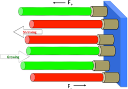
Figure 1: (Color online) Our model is depicted schematically. The wall to which the MTs are attached is represented by the blue vertical slab. The polymerizing (growing) and depolymerizing (shrinking) MTs are represented by the horizontal green cylinders (with dashed outlines) and red cylinders (with solid outlines), respectively. The grey short cylinders, into which the plus end of the MTs are inserted, represent the “couplers” that couple the MTs with the wall. The directions of polymerization and depolymerization are indicated by the double arrows. The directions of the load force (the absolute value of which is $F_{+}$) on the polymerizing MTs and load tension (the absolute value of which is $F_{-}$) on the depolymerizing MTs are indicated by the single arrows.

As we stated in the introduction, our study has been motivated partly by collective force generation by MTs during chromosome segregation. The model is depicted schematically in fig.1. At present the identity of the molecules that couple MTs to the chromosomal cargo and the detailed mechanism of force generation at the MT-cargo interface are under intense investigation mcintosh12 ; cheeseman08 . Plausible scenarios for the coupling suggested in the literature include, for example, mechanisms based on (i) biased diffusion of the coupler hill85 , (ii) power stroke on the coupler koshland88 , (iii) attachment (and detachment) of long flexible tethers zaytsev13 . Moreover, the mechanisms of the MT-cargo coupling may also vary from one species to another. Therefore, in order to maintain the generic character of our model, we neither make any explicit microscopic model for the coupler nor postulate any detailed mechanism by which the individual members of the MT bundle couple with the chromosomal cargo. This is similar, in spirit, to the kinetic models of hauling of membrane-bounded cargo where no explicit molecular mechanism is assumed for the motor-cargo coupling berger11 . The only assumption we make about the MT-wall coupling is that none of the MTs detaches from the wall during the period of our observation; catastrophe and rescue of a MT merely reverse the direction of the force that it exerts on the wall.

We assume that during the period of our observation neither nucleation of new MTs take place nor does any of the existing MTs disappear altogether because of its depolymerization. Therefore, the total number of MTs, denoted by $N$, is conserved. We use the symbols $n_{+}(t)$ and $n_{-}(t)$ to denote the MTs in the growing and shrinking phases, respectively, at time $t$ so that $n_{+}(t)+n_{-}(t)=N$. Thus, at time $t$, $n_{+}(t)$ MTs push the cargo while, simultaneously, $n_{-}(t)$ MTs pull the same cargo in the opposite direction.

As we show in this paper, the distribution of the MTs in the two groups, namely $n_{+}$ and $n_{-}$, is a crucial determinant of the nature of the movements of the wall. By carrying out computer simulations, we also monitor the displacement and velocity distribution of the wall in different regimes of the model parameters to characterize its distinct states of motility. The observed states of motility are displayed on a phase diagram.

II.1 Parameters and equations: force-dependence

The force-dependent rates of catastrophe and rescue of a MT are denoted by the symbols $c(F)$ and $r(F)$, respectively, while $c_{0}$ and $r_{0}$ refer to the corresponding values in the absence of load force. The experimental data collected over the last few years franck07 and very recent modeling sharma14 have established the dependence of the rates of catastrophe and rescue on the load force. Accordingly, we assume

$$c(F)=c_{0}~{}exp(|F|/F_{*c})$$ (1)

where $|F|$ is the absolute value of the load force opposing polymerization, and $F_{*c}$ is the characteristic force that characterizes the rapidity of variation of the catastrophe rate with the load force. Similarly, we assume

$$r(F)=r_{0}~{}exp(|F|/F_{*r})$$ (2)

where $|F|$ is the absolute value of the load tension opposing depolymerization and $F_{*r}$ is the characteristic force that characterizes the rapidity of variation of the depolymerization rate with the load force.

We denote the load-free velocities of polymerization and depolymerization of a single MT by the symbols $v_{g}$ and $v_{d}$, respectively. For the load-dependence of these velocities we follow the standard practice in the literature for modeling the load-dependence of the velocity of motor proteins. Specifically, we assume linear force-velocity relation

$$v_{+}=v_{g}\biggl{(}1-\frac{|F_{+}|}{F_{s_{+}}}\biggr{)}~{}{\rm for}~{}|F_{+}|\leq F_{s_{+}}$$ (3)

for the polymerizing MTs, and

$$v_{-}=v_{d}\biggl{(}1-\frac{|F_{-}|}{F_{s_{-}}}\biggr{)}~{}{\rm for}~{}|F_{-}|\leq F_{s_{-}}$$ (4)

for the depolymerizing MTs, where $|F_{+}|$ and $|F_{-}|$ denote the absolute values of the respective load forces opposing polymerization and depolymerization, respectively, of the corresponding MT. $F_{s_{+}}$ and $F_{s_{-}}$ are the absolute values of the stall forces corresponding to the polymerizing and depolymerizing MTs.

In the spirit of many earlier theoretical models of bidirectional transport of membrane-bounded cargo berger11 we also make the following assumptions:
(i) push on the wall by polymerizing MTs generates the indirect load tension on the depolymerizing MTs while the pull of the latter on the same wall simultaneously creates the load force against the polymerizing MTs. (ii) the load force against polymerization is shared equally by the $n_{+}(t)$ MTs, and the load tension against depolymerization is also shared equally by the $n_{-}(t)$ MTs. At any arbitrary instant of time $t$, each of the $n_{+}(t)$ polymerizing MTs attached the chromosomal cargo experiences a load force $F_{+}$ and exerts a force $-F_{+}$. Similarly, each of $n_{-}(t)$ depolymerizing MTs feels a load tension $-F_{-}$ and offers a load force $F_{-}$. Therefore, force balance on the wall attached simultaneously by $n_{+}(t)$ and $n_{-}(t)$ MT is

$$n_{+}F_{+}=-n_{-}F_{-}\equiv F_{w}(n_{+},n_{-}).$$ (5)

Equation (5), which defines the symbol $F_{w}(n_{+},n_{-})$, is just a mathematical representation of Newton’s third law: the force exerted by the wall on each MT is equal and opposite to that exerted by the same MT on the wall. According to our choice of the signs, the load force on the polymerizing MTs are positive. Based on the assumption (ii) above, we now have

$$|F_{+}(n_{+},n_{-})| = |F_{w}(n_{+},n_{-})|/n_{+}$$

$$|F_{-}(n_{+},n_{-})| = |F_{w}(n_{+},n_{-})|/n_{-}.$$ (6)

When $n_{+}(t)$ and $n_{-}(t)$ are the numbers of MTs in the polymerizing and depolymerizing phases, respectively, the corresponding catastrophe and rescue rates are

$$c_{n+,n-}(F) = c_{0}~{}exp(|F_{+}(n_{+},n_{-})|/F_{\star c})$$

$$r_{n+,n-}(F) = r_{0}~{}exp(|F_{-}(n_{+},n_{-})|/F_{\star r}),$$ (7)

respectively.

Since all the $n_{+}(t)$ polymerizing MTs and $n_{-}(t)$ depolymerizing MTs are, by definition, attached to the wall at time $t$, their velocities of growth and decay, respectively, must be identical to the wall velocity $v_{w}$, i.e.,

$$v_{w}(n_{+}(t),n_{-}(t))=v_{+}(F_{w}/n_{+}(t))=-v_{-}(-F_{w}/n_{-}(t))$$ (8)

Now substituting eqs.(6) into eqs.(3) and (4) we get

$$v_{+}=v_{g}\biggl{(}1-\frac{F_{w}}{n_{+}F_{s_{+}}}\biggr{)}$$ (9)

$$v_{-}=v_{d}\biggl{(}1-\frac{F_{w}}{n_{-}F_{s_{-}}}\biggr{)}$$ (10)

Imposing the constraint (8) on eqs. (3) and (4) we get the force

$$F_{w}(n_{+},n_{-})=\mu n_{+}F_{s_{+}}+(1-\mu)n_{-}F_{s_{-}}$$ (11)

and velocity

$$v_{w}(n_{+},n_{-})=\frac{n_{+}F_{s_{+}}-n_{-}F_{s_{-}}}{n_{+}\biggl{(}\frac{F_{s_{+}}}{v_{g}}\biggr{)}+n_{-}\biggl{(}\frac{F_{s_{-}}}{v_{d}}\biggr{)}}$$ (12)

for the wall where $\mu^{-1}=1+\frac{(n_{+}F_{s_{+}}v_{d})}{(n_{-}F_{s_{-}}v_{g})}$.

At every instant of time $t$ the state of the system is characterized by $n_{+}(t)$ and $n_{-}(t)$. The probability of finding the system in the state $n_{+}(t),n_{-}(t)$ at time $t$ is denoted by $P(n_{+},n_{-},t)$ and its time evolution is governed by the master equation

$$\frac{dP(n_{+},n_{-},t)}{dt}=$$

$$+ c_{n_{+}+1,n_{-}-1}~{}P(n_{+}+1,n_{-}-1,t)$$

$$+ r_{n_{+}-1,n_{-}+1}~{}P(n_{+}-1,n_{-}+1,t)$$

$$- (c_{n_{+},n_{-}}+r_{n_{+},n_{-}})P(n_{+},n_{-},t)$$

where $c_{n_{+},n_{-}}$ and $r_{n_{+},n_{-}}$ are given by the equations (7) while

$$c_{n_{+}+1,n_{-}-1}(F) = c_{0}~{}exp(|F_{+}(n_{+}+1,n_{-}-1)|/F_{\star c})$$

$$r_{n_{+}-1,n_{-}+1}(F) = r_{0}~{}exp(|F_{-}(n_{+}-1,n_{-}+1)|/F_{\star r}).$$

Note that the rate constants in equation (LABEL:eq-master1) depend on the time-dependent quantities $n_{+}(t)$ and $n_{-}(t)$. Therefore, the rate constants on the right hand side of eqnation (LABEL:eq-master1) take their instantaneous values at time $t$.

II.2 Comparison with other similar phenomena and models

We can now compare the model system under study here with the models of transport of membrane-bounded cargo (vesicles or organelles) by antagonistic motor proteins (e.g., kinesins and dyneins) that move on a filamentous track (e.g., a MT) chowdhury13a ; chowdhury13b . The polymerizing and depolymerizing MTs are the analogs of kinesins and dyneins. However, one crucial difference between the two situations is that unlike a MT, that can switch from polymerizing to depolymerizing phase (because of catastrophe) and from depolymerizing to polymerizing phase (because of rescue), interconversion of plus and minus-end directed motor proteins is impossible.

A systematic comparison of these two systems is presented in table 1.

Object or property	Multi-MT system	Multi-motor system
Cargo	kinetochore (kt)	vesicle or organelle
Antagonistic force generators	Polymerizing MT, depolymerizing MT	kinesin, dynein
Inter conversion of force generators	Polymerizing MT ${\rightleftharpoons}$ Depolymerizing MT: possible	Kinesin ${\rightleftharpoons}$ Dynein: impossible
Total number conservation	$N_{+}(t)+N_{-}(t)=N$=constant	$N_{+}+N_{-}=N$=constant
Numbers of + and - force generators	Time-dependent $N_{+}(t)$, $N_{-}(t)$	$N_{+}$=constant, $N_{-}$=constant
Number attached to cargo	$n_{+}(t)=N_{+}(t),n_{-}(t)=N_{-}(t)$	$n_{+}(t)\leq N_{+},n_{-}(t)\leq N_{-}$
Track	No analog	MT
Rate of attachment to track	No analog	$\omega_{a}$
Rate of detachment from track	No analog	$\omega_{d}$

Table 1: Comparison of cargo hauling by bundle of parallel dynamic MTs and by antagonistic cytoskeletal motor proteins.

III Results and discussion: motility states

We have simulated the time evolution of $n_{+}(t)$ and $n_{-}(t)$, that is described by the master equation (LABEL:eq-master1) using Gillespie algorithm gillespie07 . We get the instantaneous velocity $v_{w}(n_{+},n_{-})$ by substituting the corresponding values of $n_{+}(t)$ and $n_{-}(t)$ into equation (12). This data is used not only for plotting the velocity distribution but also for computing the displacements of the wall as a function of time. Moreover, the instantaneous force $F_{w}(n_{+},n_{-})$ evaluated using (11) is used for updating $n_{+}$ and $n_{-}$ in the next time step. Finally, all the distinct states of motility of the wall are characterized by the statistics of $n_{+},n_{-}$ . For the simulation we have assumed that initially half of the MTs are in the the state of polymerization while the remaining half are in the state of depolymerization. For the presentation of our data, it would be convenient to reduce the number of parameters. Therefore, in this paper we report the results only for the cases where $v_{g}=v_{d}$, $c_{0}=r_{0}=\gamma_{0}$, $F_{s+}=F_{s-}=F_{s}$. The magnitudes of $v_{g}=v_{d}=50$ nm/s are identical in all the figures plotted below.

(A)

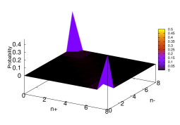
(B)

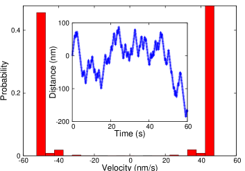
Figure 2: Characteristics of “bidirectional motion” (+-) state. (A) There are two distinct maxima in the 3D plot of the probability against the numbers of growing ($n_{+}$) and shrinking ($n_{-}$) MT; the peak near $n_{-}=0$ occurs when majority of the MTs are growing whereas the peak near $n_{+}=0$ indicates majority of the shrinking MTs. (B) The long stretches of alternate positive and negative displacements are clearly visible in the typical trajectory displayed in the inset. The two distinct and sharp peaks at the velocities $\pm 50$nm/s correspond to the two long stretches of positive and negative displacements of the wall. Numerical value of the parameters, used in the simulation are $F_{s}=6$ pN,$v_{g}=v_{d}=$50 nm/s, $c_{0}=r_{0}=10$ s^-1, and $F_{*c}=F_{*r}=3.0$ pN

(A)

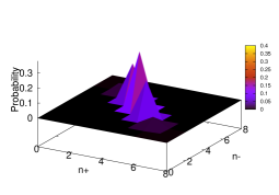
(B)

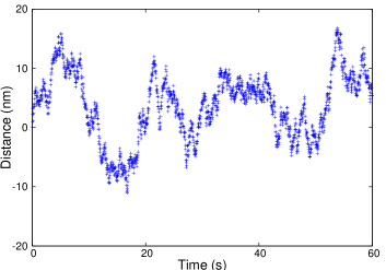
(C)

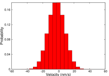
Figure 3: Characteristics of “no motion” (0) state. (A) In the 3D plot of the probability against the numbers of growing ($n_{+}$) and shrinking ($n_{-}$) MTs peaks are seen along the diagonal, i.e., $n_{+}=n_{-}$. (B) The small random positive and negative displacements of the wall recorded with the passage of time reflects the fluctuations in the position of the wall as a consequence of the tug-of-war between the growing and shrinking MTs. (C) The sharp dominant peak at zero velocity in the distribution of velocities is a signature of the ‘no motion’ state; the small non-zero probabilities at other velocities correspond to the small random excursions of the wall about its mean position. Numerical value of the parameters, used in the simulation are $F_{s}=0.1$ pN,$v_{g}=v_{d}=$50 nm/s, $F_{*c}=F_{*r}=10.0$ pN and $c_{0}=r_{0}=2000s^{-1}$.

$\bullet$ Bi-directional motion in the ‘Plus and Minus Motion (+-)’ state

First we simulated the model for the parameter values $c_{0}=r_{0}=10$ s^-1, and $F_{*c}=F_{*r}=3.0$ pN. The numerical data obtained from simulation are plotted in fig.2. In this case the typical trajectories provide direct evidence for bi-directional motion of the wall. This is also consistent with the two distinct and sharp peaks at $V=\pm 50$ nm/s in the distribution of velocities of the wall. The physical origin of this bi-directional motion berger11 can be inferred from the nature of the distribution $P(n_{+},n_{-})$ which now exhibits two maxima. The maximum at $n_{+}>0,n_{-}\simeq 0$ corresponds to the situation where the wall is driven forward almost exclusively by the growing MTs whereas that at $n_{-}>0,n_{+}\simeq 0$.

The physical origin of the bi-directional motion in this case can be understood by critically examining the interplay of the time-dependence of $n_{+}(t),n_{-}(t)$ and the dependence of $c(F),r(F)$ on $n_{+}(t),n_{-}(t)$. Although initially, $n_{+}(0)=N/2=n_{-}(0)$, stochastic nature of catastrophe and rescue causes population imbalance in spite of the equal values of the corresponding rate constants. Because of the appearance of $n_{+}(t),n_{-}(t)$ in eq.(7) the population imbalance grows further. Thus, if $n_{+}(t)$ keeps increasing with time $t$, the wall continues to move forward; eventually, if $n_{-}$ vanishes, $v_{w}$ would become identical to $v_{g}$. However, by that time, because of the non-vanishing $c_{0}$, the polymerizing MTs start suffering catastrophe that, in turn, increases population of depolymerizing MTs which has a feedback effect. Once the majority of the MTs are in the depolymerizing state the wall reverses its direction of motion. The velocity of the wall alternates between positive and negative values, corresponding to the alternate segments of the trajectory, that characterizes the bi-directional motion of the wall.

(A1)	(B1)
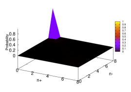
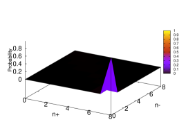
(A2)	(B2)

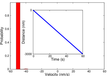
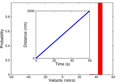
Figure 4: Characteristics of only minus and only plus motion. Numerical value of the parameters, used in the simulation are $F_{s}=5.0$ pN,$v_{g}=v_{d}=$50 nm/s,$c_{0}=r_{0}=10$ s^-1. To get only minus or only plus motion we take $F_{*c}=3.0$ pN , $F_{*r}=6.0$ pN and vice versa. (A1)Probability vs motor number plot has maxima for only shrinking MT number. Corresponding velocity distribution and displacement are shown in (A2) and inset of (A2), respectively. (B1)Probability vs motor number plot has maxima for only growing MT number. Corresponding velocity distribution and displacement are shown in (B2) and inset of (B2), respectively.

$\bullet$ Tug-of-war in the ‘No Motion (0)’ state

Next we chose the parameter values $F_{*c}=F_{*r}=10.0$ pN and $c_{0}=r_{0}=2000s^{-1}$. Note that that catastrophe and rescue rates are much higher than those in the previous case. Consequently, each MT very frequently switches between the polymerizing and depolymerizing states. Moreover, because of the much smaller values of $F_{s}$, a MT can exert very small force on the wall in both cases. The results of simulation are plotted in fig.3. The velocity distribution exhibits a single peak at zero velocity which is a signature of the ‘No Motion (0)’ state berger11 . This is a consequence of the tug-of-war between the growing and shrinking MTs that is evident in the single maximum at $n_{+}=n_{-}$ in the probability distribution $P(n_{+},n_{-})$. Tug-of-war does not mean complete stall; small fluctuations around the stall position visible in the trajectory gives rise to the non-zero width of the velocity distribution around zero velocity. The underlying physical processes in this case are almost identical to those in the case of bi-directional motion except for crucial difference arising from the relatively higher values of $c_{0}=r_{0}$; even before the wall can cover a significant distance in a particular direction the MTs reverse their velocities. Because of the high frequencies of catastrophe and rescue the wall remains practically static except for the small fluctuations about this position.

$\bullet$ Only plus (+) motion and only minus (-) motion

Finally, for the sake of completeness, we explored asymmetric behavior of the model by choosing $F_{*c}<F_{*r}$ in one case and $F_{*c}>F_{*r}$ in the other so that in one case the wall exhibits only minus motion whereas in the other case it exhibits only plus motion. The simulation results are plotted side-by-side for these two cases in fig.4. In this case the typical trajectories indicate motion either only in the plus direction or only in the minus direction. This observation is also consistent with the single sharp peaks at $V=+50$ nm/s and $V=-50$ nm/s in the distribution of velocities of the wall. The maximum at $n_{-}>0,n_{+}\simeq 0$ corresponds to the situation where the wall is driven backward almost exclusively by the shrinking MTs whereas in another case $n_{+}>0,n_{-}\simeq 0$ the wall is driven forward by the growing MTs.

$\bullet$ Phase diagram

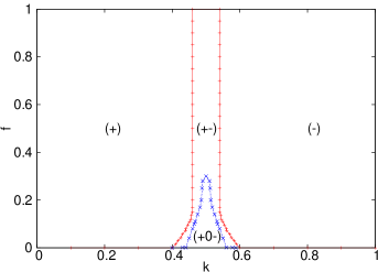
Figure 5: All the distinct states of motility of the wall for the case $F_{*c}=F_{*r}$ are displayed on the $f-k$ phase diagram (see text for the definitions of $f$ and $k$). The phases are labelled by the corresponding symbols (see text for the meaning of these symbols). The re-entrance phenomenon exhibited for $f\lesssim 0.23$ is also explained in the text.

The movement of the wall depends crucially on two important dimensionless parameters, namely, $k=c_{0}/(c_{0}+r_{0})$ and $f=F_{s}/(F_{s}+F_{\star})$. For the sake of simplicity and for reducing the number of parameters, here we have assumed $F_{*c}=F_{*r}=F_{*}$. We have varied these model parameters over wide range of values and, for each set of values, we have identified the state of movement of the wall. The corresponding observations for the symmetric case $F_{*c}=F_{*r}=F_{*}$, are summarized in fig.5 in the form of a phase diagram on the $f-k$ plane. Since no new motility state, other than those observed in the symmetric case $F_{*c}=F_{*r}$ are observed in the more general asymmetric case $F_{*c}\neq F_{*r}$, we have not drawn the higher-dimensional phase diagram.

For high force ratio ($f\gtrsim 0.23$) we observe transition from (+) to (-) region through the (+-) region in between, as the ratio $k$ is varied. In contrast, for $f\lesssim 0.23$ the system exhibits “re-entrance”; as $k$ increases from $0.4$ to $0.6$, first a transition from the motility state (+-) to the state (+0-) takes place and, at a somewhat higher value of $k$ a re-entrance to the state (+-) occurs. This re-entrance phenomenon disappears at $f\gtrsim 0.23$.

IV Summary and conclusion

In this paper we have introduced a theoretical model for studying the cargo-mediated collective kinetics of polymerization and depolymerization of a bundle of parallel MTs that are not bonded laterally with one another. Carrying out computer simulations of the model we have identified and characterized the motility states of a hard wall-like cargo that is pushed and pulled by this MT bundle that is oriented perpendicular to the plane of the wall. Among these motility states, one corresponds to “no motion” (except for small fluctuations); it arises from the “tug-of-war” between the polymerizing and depolymerizing MTs. The wall exhibits a bi-directional motion in another motility state. The qualitative features of the characteristics of this bi-directional state of motility of the wall are similar to those observed in bi-directional motion of vesicular cargo driven by antagonistic motor proteins. But, as we have argued here, the physical origin of the bidirectional motion in these two systems are completely different. In the case of motor protein-driven vesicular cargo the bi-directional motion is caused by an interplay of the stall force of the motors and the load-dependent detachment of the motor from its track berger11 . In contrast, in our model of MT-driven wall, the bi-directional motion arises from a subtle interplay of the stall force of the MTs and the load-dependent depolymerization of the MTs. This result should be regarded also as a “proof-of-principle” that for bi-directional motion of the chromosomal cargo active participation motor proteins is not essential; in contrast to past claims in the literature (see ref.sutradhar14 for a very recent claim), the polymerization / depolymerization kinetics of the MTs are adequate to cause bidirectional motion provided the load-dependence of their rates are properly taken into account. The latter principle will be elaborated further elsewhere ghanti14b in the context of chromosome segregation with a more detailed theoretical model which also treats the kinetochore wall as a soft elastic object zelinski13 .

References

- (1) J. Howard, Mechanics of motor proteins and the cytoskeleton, (Sinauer Associates, Sunderland, 2001).
- (2) A. Desai and T.J. Mitchison, Annu. Rev. Cell Dev. Biol. 13, 83 (1997).
- (3) L. Laan, J. Husson, E. L. Munteanu, J. W. J. Kerssemakers, and M. Dogterom, PNAS, 105, 26 (2008).
- (4) G. Oster and A. Mogilner, in: Supramoleculr polymers, (ed.) A. Ciferri (Dekker, 2004).
- (5) T. Kühne, R. Lipowsky and J. Kierfeld, EPL 86, 68002 (2009).
- (6) J. Krawczyk and J. Kierfeld, EPL 93, 28006 (2011).
- (7) C.S. Peskin and G.F. Oster, Biophys. J. 69, 2268 (1995).
- (8) J.R. McIntosh, V. Volkov, F.I. Ataullakhanov and E.L. Grischuk, J. Cell Sci. 123, 3425 (2010).
- (9) D. Chowdhury, Phys. Rep. 529, 1 (2013).
- (10) D. Chowdhury, Biophys. J. 104, 2331 (2013).
- (11) A. B. Kolomeisky, J. Phys. Condens. Matt. 25, 463101 (2013).
- (12) J.R. McIntosh, M.I. Molodtsov and F.I. Ataullakhanov, Quart. Rev. Biophys. 45, 147-207 (2012).
- (13) S. P. Gross, Phys. Biol. 1, R1 (2004).
- (14) M.A. Welte, Curr. Biol. 14, R525 (2004).
- (15) F. Berger, C. Keller, M.J.I. Müller, S. Klumpp and R. Lipowsky, Biochem. Soc. Trans. 39, 1211 (2011).
- (16) D. Ghanti and D. Chowdhury, to be published (2014).
- (17) I.M. Cheeseman and A. Desai, Nat. Rev. Mol. Cell Biol. 9, 33 (2008).
- (18) T.L. Hill, PNAS 82, 4404 (1985).
- (19) D.E. Koshland, T.J. Mitchison and M.W. Kirschner, Nature 331, 499 (1988).
- (20) A.V. Zaytsev, F.I. Ataullakhanov and E.L. Grischuk, Cell. Mol. Bioengg. 6, 393 (2013).
- (21) A. D. Franck, A. F. Powers, D. R. Gestaut, T. Gonen, T. N. Davis, C. L. Asbury, Nat. Cell Biol 9, 832 (2007).
- (22) A.K. Sharma, B. Shtylla and D. Chowdhury, Phys. Biol. 11, 036004 (2014).
- (23) D.T. Gillespie, in: Annu. Rev. Phys. Chem. 58, 35 (2007).
- (24) S. Sutradhar and R. Paul, J. Theor. Biol. 344, 56 (2014).
- (25) B. Zelinski and J. Kierfeld, Phys. Rev. E 87, 012703 (2013).