Identification of core-periphery structure in networks

Abstract

Many networks can be usefully decomposed into a dense core plus an outlying, loosely-connected periphery. Here we propose an algorithm for performing such a decomposition on empirical network data using methods of statistical inference. Our method fits a generative model of core–periphery structure to observed data using a combination of an expectation–maximization algorithm for calculating the parameters of the model and a belief propagation algorithm for calculating the decomposition itself. We find the method to be efficient, scaling easily to networks with a million or more nodes and we test it on a range of networks, including real-world examples as well as computer-generated benchmarks, for which it successfully identifies known core–periphery structure with low error rate. We also demonstrate that the method is immune from the detectability transition observed in the related community detection problem, which prevents the detection of community structure when that structure is too weak. There is no such transition for core–periphery structure, which is detectable, albeit with some statistical error, no matter how weak it is.

I Introduction

Much of the recent work on the structure of networked systems, such as social and technological networks, has focused on measurements of local structure, such as vertex degrees, clustering coefficients, correlations, and so forth Boccaletti et al. (2006); Newman (2010). Increasingly, however, researchers have investigated medium- and large-scale structure as well. The lion’s share of the attention has gone to the study of so-called community structure Fortunato (2010), the archetypal example of large-scale network structure, in which the nodes of a network are divided into tightly knit groups or communities that often reflect aspects of network function. But other structure types can be important as well and recent research has also looked at overlapping or fuzzy communities Palla et al. (2005); Airoldi et al. (2008); Ahn et al. (2010), hierarchical structure Ravasz and Barabási (2003); Clauset et al. (2008), and ranking Ball and Newman (2013), among others.

In this paper we focus on another, distinct type of large-scale structure, core–periphery structure. Many networks are observed to divide into a densely interconnected core surrounded by a sparser halo or periphery. Already in the 1990s sociologists observed such structure in social networks Borgatti and Everett (1999) and more recently a number of researchers have made quantitative studies of core–periphery structure in a range of different types of networks Holme (2005); Rombach et al. (2014). The identification of core–periphery structure has a number of potential uses. Core nodes in a network might play a different role from peripheral ones Guimerà and Amaral (2005) and the ability to distinguish core from periphery might thus give us a new handle on function in networked systems. Distinguishing between core and periphery might lead to more informative visualizations of networks or find a role in graph layout algorithms similar to that played today by community structure. And core nodes, for instance in social networks, might be more influential or powerful than peripheral ones, so the ability to discern the difference could shed light on social or other organization.

There have also been studies of two other types of structure that are reminiscent of, though different in important ways from, core–periphery structure: “rich club” structure Colizza et al. (2006); Zhou and Mondragon (2004) and degree assortativity Pastor-Satorras et al. (2001); Newman (2002). A rich-club is a group of high-degree nodes in a network (i.e., nodes with many connections to others) that preferentially connect to one another. Such a club is a special case of the core in a core–periphery structure, but the concept of a core is more general, encompassing cases (as we will see) in which low-degree nodes can also belong to the core. The rich-club phenomenon also makes no statement about connectivity patterns in the remainder of the network, where as core–periphery structure does.

Assortative mixing is the tendency of nodes in a network to connect to others that are similar to themselves in some way, and degree-assortative mixing is the tendency to connect to others with similar degree—high to high, and low to low. This produces a core in the network of connected high-degree vertices, similar to the rich-club, but low-degree vertices also preferentially connect to one another and prefer not to connect to the core, which is the opposite of core–periphery structure as commonly understood, in which periphery vertices are more likely to connect to the core than they are to one another.

A number of suggestions have been made about how, given the complete pattern of connections in a network, one could detect core–periphery structure in that pattern. All of them take the same basic approach of defining an objective function that measures the strength or quality of a candidate division into core and periphery and then maximizes (usually only approximately) over divisions to find the best one. In early work, Borgatti and Everett Borgatti and Everett (1999) proposed a quality function based on comparing the network to an ideal core–periphery model in which nodes are connected to each other if and only if they are members of the core. Rombach et al. Rombach et al. (2014) built on the same idea, but using a more flexible model. Holme Holme (2005) took a contrasting approach reminiscent of the clustering coefficient used to quantify transitivity in networks.

In this paper we propose a different, statistically principled method of detecting core–periphery structure using a maximum-likelihood fit to a generative network model. The method is conceptually similar to recently-popular first-principles methods for community detection Bickel and Chen (2009); Decelle et al. (2011a) and in fact uses the same underlying network model, the stochastic block model, although with a different choice of parameters appropriate to core–periphery rather than community structure. Among other results we demonstrate that the method is able consistently to detect planted core–periphery structure in computer-generated test networks, and that, by contrast with the community detection problem, there is no minimum amount of structure that can be detected. Any core–periphery structure, no matter how weak, is in principle detectable.

II The stochastic block model

The stochastic block model is a well established and widely used model for community structure in networks. It is a generative model, meaning its original purpose is to create artificial networks that contain community structure. It is also commonly used, however, for community detection by fitting the model to observed network data. The parameters of the fit tell us the best division of the network into communities.

The model is defined as follows. We take $n$ nodes, initially without any edges connecting them, and divide them into some number of groups. We will consider the simplest case where there are just two groups (which will represent the core and periphery). Each vertex is assigned randomly to group 1 with probability $\gamma_{1}$ or group 2 with probability $\gamma_{2}=1-\gamma_{1}$. Then between every vertex pair we place an undirected edge independently at random with probability $p_{rs}$, or not with probability $1-p_{rs}$, where $r$ and $s$ are the groups to which the two vertices belong. Thus the probability of connection of any two vertices depends solely on their group membership. The probabilities $p_{rs}$ form a matrix, sometimes called the mixing matrix or affinity matrix, which is a $2\times 2$ matrix in our two-group example. Since the edges in the network are undirected it follows that the mixing matrix is symmetric, $p_{12}=p_{21}$, leaving three independent probabilities that we can choose, $p_{11}$, $p_{12}$, and $p_{22}$.

In the most commonly studied case the probabilities for connection within groups are chosen to be larger than the probabilities between groups $p_{11}>p_{12}<p_{22}$. This gives traditional community structure, also called assortative mixing, with denser connections within groups than between them. A contrasting possibility is the disassortative choice $p_{11}<p_{12}>p_{22}$, where edges are more probable between groups than within them. This choice, and the structure it describes, has received a modest amount of attention in the literature Newman (2003); Yan et al. (2011).

There is, however, a third possibility that has rarely been studied, in which $p_{11}>p_{12}>p_{22}$. This is the situation we refer to as core–periphery structure. Since the group labels are arbitrary we can, without loss of generality, assume $p_{11}$ to be the largest of the three probabilities, so group 1 is the core. Connections are most probable within the core, least probable within the periphery, and of intermediate probability between core and periphery. Note that this means that periphery vertices are more likely to be connected to core vertices than to each other, a characteristic feature of core–periphery structure that distinguishes it from either assortative or disassortative mixing.

As we have said, the stochastic block model can be used to detect structure in network data by fits of the data to the model. For instance, the assortative version of the model can be used to fit and hence detect community structure in networks Bickel and Chen (2009); Decelle et al. (2011a). As shown in Karrer and Newman (2011), however, it often performs poorly at this task in real-world situations because real-world networks tend to have broad degree distributions that dominate the large-scale structure and the fit tends to pick out this gross effect rather than the more subtle underlying community structure—typically the fit just ends up dividing the network into groups of higher- and lower-degree vertices rather than traditional communities. A more nuanced view has been given by Decelle et al. Decelle et al. (2011b), who show that in fact both the degree-based division and the community division are good fits to the model—local maxima of the likelihood in the language introduced below—but the degree-based one is better.

But when we turn to core–periphery structure this bug becomes a feature. In networks with core–periphery structure the vertices in the core typically do have higher degree than those in the periphery, so a method that recognizes this fact is doing the right thing. Indeed, as we show in Section V, one can in certain cases do a reasonable job of detecting core–periphery structure just by separating vertices into two groups according to their degrees. On the other hand, one can do better still using the stochastic block model.

III Fitting to empirical data

We propose to detect core–periphery structure in networks by finding the parameters of the stochastic block model that best fit the model to a given observed network. This we do by the method of maximum likelihood, implemented using an expectation–maximization or EM algorithm Dempster et al. (1977). The use of EM algorithms for network model fitting is well established Nowicki and Snijders (2001); Newman and Leicht (2007), but it is worth briefly running through the derivation for our particular model, which goes as follows.

III.1 The EM algorithm

Given a network, the question we ask is, if this network were generated by the stochastic block model, what is our best guess at the values of the parameters of that model? To answer this question, let $A_{ij}$ be an element of the adjacency matrix $A$ of the network having value one if there is an edge between vertices $i$ and $j$ and zero otherwise, and let $g_{i}$ be the group that vertex $i$ belongs to. Then the probability, or likelihood, that the network was generated by the model is

$$P(A|p,\gamma) =\sum_{g}P(A|p,\gamma,g)P(g|\gamma)$$

$$=\sum_{g}\prod_{i<j}p_{g_{i}g_{j}}^{A_{ij}}(1-p_{g_{i}g_{j}})^{1-A_{ij}}\prod_{i}\gamma_{g_{i}},$$ (1)

where $\sum_{g}$ indicates a sum over all assignments of the vertices to groups.

To determine the most likely values of the parameters $p_{rs}$ and $\gamma_{r}$, we maximize this likelihood with respect to them. In fact it is technically simpler to maximize the logarithm of the likelihood:

$$\log P(A|p,\gamma)=\log\sum_{g}\prod_{i<j}p_{g_{i}g_{j}}^{A_{ij}}(1-p_{g_{i}g_{j}})^{1-A_{ij}}\prod_{i}\gamma_{g_{i}},$$ (2)

which is equivalent since the logarithm is a monotone increasing function. Direct maximization is still quite difficult, however. Simply differentiating to find the maximum leads to a complex set of implicit equations that have no easy solution.

A better approach, and the one taken in the EM algorithm, involves the application of Jensen’s inequality, which says that for any set of positive-definite quantities $x_{i}$

$$\log\sum_{i}x_{i}\geq\sum_{i}q_{i}\log{x_{i}\over q_{i}},$$ (3)

where $q_{i}$ is any probability distribution satisfying the normalization condition $\sum_{i}q_{i}=1$. One can easily verify that the exact equality is achieved by choosing

$$q_{i}=x_{i}/\sum_{i}x_{i}.$$ (4)

For any properly normalized probability distribution $q(g)$ over the group assignments $g$, Jensen’s inequality applied to Eq. (2) gives

$$\log P(A|p,\gamma) \geq\sum_{g}q(g)\log\biggl{[}{1\over q(g)}\prod_{i<j}p_{g_{i}g_{j}}^{A_{ij}}(1-p_{g_{i}g_{j}})^{1-A_{ij}}\prod_{i}\gamma_{g_{i}}\biggr{]}$$

$$=\sum_{g}q(g)\biggl{[}\sum_{i<j}\bigl{[}A_{ij}\log p_{g_{i}g_{j}}+(1-A_{ij})\log(1-p_{g_{i}g_{j}})\bigr{]}+\sum_{i}\log\gamma_{g_{i}}-q(g)\log q(g)\biggr{]}$$

$$=\frac{1}{2}\sum_{ij}\sum_{rs}\bigl{[}A_{ij}q_{rs}^{ij}\log p_{rs}+(1-A_{ij})q_{rs}^{ij}\log(1-p_{rs})\bigr{]}+\sum_{ir}q_{r}^{i}\log\gamma_{r}-\sum_{g}q(g)\log q(g),$$ (5)

where $q_{r}^{i}$ is the so-called marginal probability within the chosen distribution $q(g)$ that vertex $i$ belongs to group $r$:

$$q_{r}^{i}=\sum_{g}q(g)\delta_{g_{i},r},$$ (6)

and $q_{rs}^{ij}$ is the joint or two-vertex marginal probability that vertex $i$ belongs to group $r$ and vertex $j$ simultaneously belongs to group $s$:

$$q_{rs}^{ij}=\sum_{g}q(g)\delta_{g_{i},r}\delta_{g_{j},s},$$ (7)

with $\delta_{ij}$ being the Kronecker delta.

Following Eq. (4), the exact equality in (5) is achieved when

$$q(g)={\prod_{i<j}p_{g_{i}g_{j}}^{A_{ij}}(1-p_{g_{i}g_{j}})^{1-A_{ij}}\prod_{i}\gamma_{g_{i}}\over\sum_{g}\prod_{i<j}p_{g_{i}g_{j}}^{A_{ij}}(1-p_{g_{i}g_{j}})^{1-A_{ij}}\prod_{i}\gamma_{g_{i}}}.$$ (8)

Thus calculating the maximum of the left-hand side of (5) with respect to the parameters $p,\gamma$ is equivalent to first maximizing the right-hand side with respect to $q(g)$ (by choosing the value above) so as to make the two sides equal, and then maximizing the result with respect to the parameters. In this way we turn our original problem of maximizing over the parameters into a double maximization of the right-hand side expression over the parameters and the distribution $q(g)$. At first glance, this would seem to make the problem more difficult, but numerically it is in fact easier, since it splits a challenging maximization into two separate and relatively elementary operations. The maximization with respect to the parameters is achieved by straightforward differentiation of (5) with the constraint that $\sum_{r}\gamma_{r}=1$. Note that the final term on the right-hand side does not depend on the parameters and hence vanishes upon differentiation, and we arrive at the following expressions for the parameters:

$$p_{rs} ={\sum_{ij}A_{ij}q_{rs}^{ij}\over\sum_{ij}q_{rs}^{ij}},$$ (9)

$$\gamma_{r} ={1\over n}\sum_{i}q_{r}^{i},$$ (10)

where $n$ is the total number of vertices as previously. The simultaneous solution of Eqs. (8) to (10) now gives us the optimal values of the parameters.

The EM algorithm solves these equations by numerical iteration. Given an initial guess at the parameters $p$ and $\gamma$ we can calculate the probability distribution $q(g)$ from Eq. (8) and from it the one- and two-vertex marginal probabilities, Eqs. (6) and (7). And from these we can calculate a new estimate of $p$ and $\gamma$ from Eqs. (9) and (10). It can be proved that upon iteration this process will always converge to a local maximum of the log-likelihood. It may not be the global maximum, however, so commonly one performs the entire calculation several times with different starting conditions, choosing from among the solutions so obtained the one with the highest likelihood.

Equation (9) can be simplified a little further by using Eq. (7) to rewrite the denominator thus:

$$\sum_{ij}q_{rs}^{ij}=\sum_{g}q(g)\sum_{i}\delta_{g_{i},r}\sum_{j}\delta_{g_{j},s}=\left\langle n_{r}n_{s}\right\rangle,$$ (11)

where $\left\langle\ldots\right\rangle$ indicates an average within the probability distribution $q(g)$ and $n_{r}=\sum_{i}\delta_{g_{i},r}$ is the number of vertices in group $r$. In the limit of large network size the number of vertices in a group becomes narrowly peaked and we can replace $\left\langle n_{r}n_{s}\right\rangle$ by $\left\langle n_{r}\right\rangle\left\langle n_{s}\right\rangle$ with

$$\left\langle n_{r}\right\rangle=\sum_{g}q(g)\sum_{i}\delta_{g_{i},r}=\sum_{i}q_{r}^{i},$$ (12)

where we have used Eq. (6). Then

$$p_{rs}={\sum_{ij}A_{ij}q_{rs}^{ij}\over\sum_{i}q_{r}^{i}\sum_{j}q_{s}^{j}}.$$ (13)

This expression has the advantage of requiring only a sum over edges in the numerator (since one need sum only those terms for which $A_{ij}=1$) and single sums over vertices in the denominator, not the double sum in the denominator of (9). This makes evaluation of $p_{rs}$ significantly faster for large networks. (Note, however, that despite appearances, Eq. (13) does not assume that $q_{rs}^{ij}=q_{r}^{i}q_{s}^{j}$, which would certainly not be correct in general. Only the sum over all vertex pairs factorizes, not the individual terms.)

The final result of the EM algorithm gives us not only the values of the parameters, but also the marginal probabilities $q_{r}^{i}$ for vertices to belong to each group. In fact, it is normally this latter quantity that we are really interested in. In the community structure context it gives the probability that vertex $i$ belongs to community $r$. In the core–periphery case, it gives the probability that the vertex belongs to either the core (group 1) or the periphery (group 2). Typically, the last step in the calculation is to assign each vertex to the group for which it has highest probability of membership, producing the final division of the network into core and periphery.

III.2 Belief propagation

The EM algorithm is an elegant approach but it has its shortcomings. Principal among them is the difficulty of performing the sum over group assignments $g$ in the denominator of Eq. (8). Even for the current case where there are just two groups, this sum has $2^{n}$ terms and would take prohibitively long to perform numerically for any but the smallest of networks. The most common way around this problem is to make an approximate estimate of the sum by Monte Carlo sampling, but in this paper we employ an alternative technique proposed by Decelle et al. Decelle et al. (2011a, b), which uses belief propagation. This technique is of interest both because it is significantly faster than Monte Carlo and also because it lends itself to further analysis, as discussed in Section IV.

Belief propagation Pearl (1988), a generalization of the Bethe–Peierls iterative method for the solution of mean-field models Bethe (1935); Peierls (1936), is a message-passing technique for finding probability distributions on networks, which we can use in this case to find the distribution $q(g)$ of Eq. (8). We define a “message” $\eta_{r}^{i\to j}$, which is equal to the probability that vertex $i$ belongs to group $r$ if vertex $j$ is removed from the network. The removal of $j$ allows one to derive a set of self-consistent of equations that must be satisfied by these messages Decelle et al. (2011a). The equations are particularly simple for the case of a sparse network where $p_{rs}$ is small so that terms of order $p_{rs}$ can be ignored by comparison with terms of order 1, which appears to describe most real-world networks. For this case, the equations are

$$\eta_{r}^{i\to j}={\gamma_{r}\over Z_{i\to j}}\prod_{k}\biggl{[}1-\sum_{s}q_{s}^{k}p_{rs}\biggr{]}\prod_{\begin{subarray}{c}k(\neq j)\\ A_{ik}=1\end{subarray}}\sum_{s}\eta_{s}^{k\to i}p_{rs},$$ (14)

where $Z_{i\to j}$ is a normalizing constant whose value is chosen to ensure that $\sum_{r}\eta_{r}^{i\to j}=1$ thus:

$$Z_{i\to j}=\sum_{r}\gamma_{r}\prod_{k}\biggl{[}1-\sum_{s}q_{s}^{k}p_{rs}\biggr{]}\prod_{\begin{subarray}{c}k(\neq j)\\ A_{ik}=1\end{subarray}}\sum_{s}\eta_{s}^{k\to i}p_{rs}.$$ (15)

Equation (14) is typically solved numerically, by starting from a random initial condition and iterating to convergence. In addition to calculating new values for the messages $\eta_{r}^{i\to j}$ on each step of this iteration we also need to calculate new values for the one-vertex marginal probabilities $q_{r}^{i}$, which satisfy

$$q_{r}^{i}={\gamma_{r}\over Z_{i}}\prod_{k}\biggl{[}1-\sum_{s}q_{s}^{k}p_{rs}\biggr{]}\prod_{\begin{subarray}{c}k\\ A_{ik}=1\end{subarray}}\sum_{s}\eta_{s}^{k\to i}p_{rs},$$ (16)

with $Z_{i}$ being another normalization constant:

$$Z_{i}=\sum_{r}\gamma_{r}\prod_{k}\biggl{[}1-\sum_{s}q_{s}^{k}p_{rs}\biggr{]}\prod_{\begin{subarray}{c}k\\ A_{ik}=1\end{subarray}}\sum_{s}\eta_{s}^{k\to i}p_{rs}.$$ (17)

Equation (14) is strictly true only on networks that are trees or are locally tree-like, meaning that in the limit of large network size the neighborhood of any vertex looks like a tree out to arbitrarily large distances. The stochastic block model itself generates networks that are locally tree-like, but many real-world networks are not, meaning that the belief-propagation method is only approximate in those cases. In practice, however, it appears to give good results, comparable in quality with those from Monte Carlo sampling (which is also an approximate method).

Once the belief propagation equations have converged, we can use the results to evaluate Eq. (13). This requires values of the two-vertex marginals, which are given by Bayes theorem to be

$$q_{rs}^{ij} =P(g_{i}=r,g_{j}=s|A_{ij}=1)$$

$$={P(g_{i}=r,g_{j}=s)\over P(A_{ij}=1)}P(A_{ij}=1|g_{i}=r,g_{j}=s),$$ (18)

where all elements of the adjacency matrix other than $A_{ij}$ are assumed given in each probability. In terms of our other variables we have

$$P(g_{i}=r,g_{j}=s) =\eta_{r}^{i\to j}\eta_{s}^{j\to i},$$

$$P(A_{ij}=1|g_{i}=r,g_{j}=s) =p_{rs},$$ (19)

and the normalization $P(A_{ij})$ is fixed by the requirement that $q_{rs}^{ij}$ sum to unity. So

$$q_{rs}^{ij}={\eta_{r}^{i\to j}\eta_{s}^{j\to i}p_{rs}\over\sum_{rs}\eta_{r}^{i\to j}\eta_{s}^{j\to i}p_{rs}}.$$ (20)

Substituting the values of $q_{r}^{i}$ and $q_{rs}^{ij}$ into Eqs. (10) and (13) then completes the EM algorithm.

Note that there are now two entirely separate iterative sections of our calculation: the EM algorithm, which consists of the iteration of Eqs. (8), (10), and (13), and the belief propagation algorithm, which consists of the iteration of Eq. (14).

Using the belief propagation algorithm is far faster than calculating $q(g)$ directly from Eq. (8). Equations (14) to (17) require the evaluation of only $\mathrm{O}(m+n)$ terms for a network with $n$ vertices and $m$ edges, meaning an iteration takes linear time in the common case of a sparse network with $m\propto n$. There is still the issue of how many iterations are needed for convergence, for which there are no firm results at present, but heuristic arguments suggest that $\mathrm{O}(\log n)$ iterations will be needed on a typical network.

The complete algorithm for detecting core–periphery structure in networks consists of the following steps:

1. Make an initial random guess at the values of the parameters $p,\gamma$.

2. From a random initial condition, iterate to convergence the belief propagation equations (14) for vertex pairs connected by an edge and the one-vertex marginal probabilities, Eq. (16).

3. Use the converged values to calculate the two-vertex marginal probabilities, Eq. (20).

4. Use the one- and two-vertex probabilities to calculate an improved estimate of the parameters from Eqs. (10) and (13).

5. Repeat from step 2 until the parameters converge.

6. Assign each vertex to either the core or the periphery, whichever has the higher probability $q_{r}^{i}$.

IV Detectability

One of the most intriguing aspects of the community detection problem is the detectability threshold Reichardt and Leone (2008); Decelle et al. (2011a); Hu et al. (2012). When a network contains strong community structure—when there is a clear difference in density between the in-group and out-group connections—then that structure is easy to detect and a wide range of algorithms will do a good job. When structure becomes sufficiently weak, however, at least in simple models of the problem such as the stochastic block model, it becomes undetectable. In this weak-structure regime it is rigorously provable that no algorithm can identify community memberships with success any better than a random coin toss Mossel et al. (2012, 2013). Given the strong connection between community detection and the core–periphery detection problem studied here, it is natural to ask whether there is a similar threshold for the core–periphery problem. Is there a point at which core–periphery structure becomes so weak as to be undetectable by our method or any other?

At the most naive level, the answer to this question is no. The core–periphery problem differs from the community detection problem in that the vertices in the core have higher degree on average than those in the periphery and hence one can use the degrees to identify the core and periphery vertices with an average success rate better than a coin toss.

Consider in particular the common case of a stochastic block model where

$$p_{rs}={c_{rs}\over n}$$ (21)

for some constants $c_{rs}$. This is the case for which the detectability threshold mentioned above is observed. Then the average degrees in the core and periphery are, respectively,

$$\bar{d}_{1}=\gamma_{1}c_{11}+\gamma_{2}c_{12},\qquad\bar{d}_{2}=\gamma_{1}c_{12}+\gamma_{2}c_{22},$$ (22)

and the difference is $\bar{d}_{1}-\bar{d}_{2}=\gamma_{1}(c_{11}-c_{12})+\gamma_{2}(c_{12}-c_{22})$. Since, by hypothesis, $c_{11}>c_{12}>c_{22}$, this quantity is always positive and $\bar{d}_{1}>\bar{d}_{2}$. Because the edges in the network are independent, the actual degrees have a Poisson distribution about the mean in the limit of large $n$, and hence the degree distribution consists of two overlapping Poisson distributions, as sketched in Fig. 1. By simply dividing the vertices according to their observed degrees, therefore, we can (on average) classify them as core or periphery with success better than chance. (This assumes we know the sizes of the two groups, which we usually don’t, but this problem can be solved—see Section IV.1.)

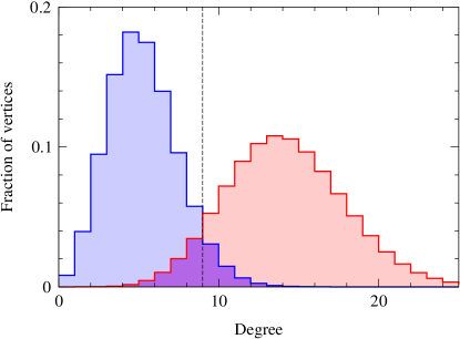
Figure 1: In the stochastic block model both core (red) and periphery (blue) vertices have Poisson degree distributions, but the mean degree is higher in the core than in the periphery, so the overall degree distribution of the network is a sum of two overlapping Poisson distributions as shown here. A simple division of vertices by degree (vertical dashed line) classifies most vertices into the correct groups, red in the core and blue in the periphery. Only those in the overlap (shown in purple) are classified incorrectly.

So rather than asking whether our ability to detect structure fails completely in the weak-structure limit, we should instead ask whether we can do any better than simply dividing vertices according to degree. The answer to this question is both yes and no. As we now show, in the limit of weak structure no algorithm can do better than one that looks at degrees only, but for stronger structure we can do better in most cases.

To demonstrate these results, we take a standard approach from statistics and ask whether our detection algorithm based on the stochastic block model can detect core–periphery structure in networks that are themselves generated using the stochastic block model. This is a so-called consistency test and, in addition to providing a well-controlled test of our algorithm, it has one very important advantage. It is known that on average the best way to detect the structure in a data set generated by a model is to perform a maximum-likelihood fit to that same model, exactly as our algorithm does. No other algorithm will return better performance on this test, on average, than the maximum likelihood method.

Bearing this in mind, consider applying the algorithm of this paper to a network generated using the stochastic block model with two equally sized groups ($\gamma_{1}=\gamma_{2}=\frac{1}{2}$) and weak core–periphery structure of the form

$$c_{11}=c+\alpha_{1}\delta,\quad c_{12}=c,\quad c_{22}=c-\alpha_{2}\delta,$$ (23)

where $\alpha_{1}$, $\alpha_{2}$, and $c$ are $\mathrm{O}(1)$ positive constants and $\delta$ is a small quantity. In the limit as $\delta\to 0$ the core–periphery structure vanishes and the network becomes a uniform random graph of average degree $c$. For small values of $\delta$ the structure is weak and it is this regime that we’re interested to probe.

To make the problem as simple as possible, suppose that we allow our algorithm to use the exact values of the parameters $\gamma_{r}$ and $p_{rs}$, meaning that we need only perform the belief propagation part of the calculation to derive an answer. There is no need to perform the EM algorithm iteration as well, since this is only needed to determine the parameters. This is a somewhat unrealistic situation—in practical cases we do not normally know the values of the parameters. However, if, as we will show, the algorithm performs poorly in this situation then it will surely perform no better if we give it less information—if we do not know the values of the parameters. Thus this choice gives us a best-case estimate of the performance of the algorithm.

To gain a theoretical understanding of how the belief propagation process works, we consider the odds ratio $q_{1}^{i}/q_{2}^{i}$ between the probabilities that a vertex belongs to the core and the periphery. Making use of Eq. (16), expanding the first product to leading order in $p_{rs}=c_{rs}/n$, and dividing top and bottom in the second product by a factor of $n$, this quantity is given by

$${q_{1}^{i}\over q_{2}^{i}}={\gamma_{1}\over\gamma_{2}}\,\mathrm{e}^{\bar{d}_{2}-\bar{d}_{1}}\!\prod_{\begin{subarray}{c}k\\ A_{ik}=1\end{subarray}}{\eta_{1}^{i\to j}c_{11}+\eta_{2}^{i\to j}c_{12}\over\eta_{1}^{i\to j}c_{12}+\eta_{1}^{i\to j}c_{22}},$$ (24)

where $\bar{d}_{1}$ and $\bar{d}_{2}$ are defined as in Eq. (22) and we have made use of Eq. (10). Note how the normalization $Z_{i\to j}$ also cancels, making calculations simpler.

Now we substitute for $c_{rs}$ from Eq. (23), set $\gamma_{1}=\gamma_{2}=\frac{1}{2}$, and note that as $\delta\to 0$ the probabilities of any vertex being in one group or the other become equal, so that

$${\eta_{1}^{i\to j}\over\eta_{2}^{i\to j}}=1+\beta_{i\to j}\delta$$ (25)

to leading order for some constant $\beta_{i\to j}$. Keeping terms to first order in $\delta$, we then find that

$${q_{1}^{i}\over q_{2}^{i}}=1+\tfrac{1}{2}(\alpha_{1}+\alpha_{2}){k_{i}-c\over c}\delta,$$ (26)

where $k_{i}$ is the degree of vertex $i$ as previously.

Note that $\beta_{i\to j}$ has dropped out of this expression, meaning that when $\delta$ is small and the structure is weak the probabilities depend only on the degree $k_{i}$ of the vertex and not on any other properties of the network structure. More specifically, vertex $i$ has a higher probability of belonging to group 1, i.e., the core, whenever its degree $k_{i}$ is greater than the average degree $c$ in the network as a whole. When its degree is below average the vertex has a higher probability of belonging to the periphery. Thus a simple division based on probabilities is precisely equivalent to dividing based on degree. Moreover, since, as we have said, no other algorithm can do better at distinguishing the structure, it immediately follows that there is nothing better one can do in the weak-structure limit than divide the vertices based on degree.

Paradoxically, the same is also true in the limit of strong structure. If the core–periphery structure is strong, meaning that there is a big difference between connection probabilities for core and periphery vertices, then the two Poisson distributions of Fig. 1 will be far apart, with very little overlap, and vertices can be accurately classified by degree alone. The means of the two distributions are $\mu_{1}=\frac{1}{2}(c_{11}+c_{12})$ and $\mu_{2}=\frac{1}{2}(c_{12}+c_{22})$ and, since the width of a Poisson distribution scales as the square root of its mean, we will have easily distinguishable peaks provided $\mu_{1}-\mu_{2}\gg\sqrt{\smash[b]{(\mu_{1}+\mu_{2})/2}}$, or

$$c_{11}-c_{22}\gg 2\sqrt{c},$$ (27)

where $c=\frac{1}{2}(\mu_{1}+\mu_{2})$ is the average degree of the network as a whole.

In fact, even between the limits of strong and weak structure there are some networks for which a simple division by degrees is optimal. Consider the two-parameter family of models defined by

$$c_{11}=\theta r,\quad c_{12}=\theta,\quad c_{22}={\theta\over r},$$ (28)

for any choice of $\gamma_{r}$, where $\theta>0$ and $r>1$. Substituting this choice into Eq. (24) gives

$${q_{1}^{i}\over q_{2}^{i}}={\gamma_{1}\over\gamma_{2}}\,\mathrm{e}^{\bar{d}_{2}-\bar{d}_{1}}r^{k_{i}},$$ (29)

so again the results depend only on the vertex degrees.

So are there any cases where we can do better than the algorithm that looks at degrees only? The answer is yes: for structure of intermediate strength, neither exceptionally weak nor exceptionally strong, and away from the plane in parameter space defined by Eq. (28), the messages are not simple functions of degree but depend in general on the details of the network structure. Since, once again, the belief propagation algorithm is optimal, it follows that any algorithm that gives a result different from the belief propagation algorithm must give an inferior one, including an algorithm that looks at degrees only. Hence in this regime one can do better than simply looking at vertex degrees. Moreover, this regime contains most cases of real-world interest. After all, core–periphery structure so weak as to be barely detectable is presumably not of great interest, and real-world networks rarely have strongly bimodal degree distributions of the kind considered above that make degree-based algorithms work well in the strong-structure limit.

There is also, we note, no evidence in this case of a detectability threshold or similar sharp discontinuity in the behavior of the algorithm. Everywhere in the parameter space the algorithm can identify core and periphery with performance better than chance.

IV.1 Degree-based algorithm

We are now also in a position to answer a question raised parenthetically in Section III.2. If we choose to classify vertices based on degree alone, what size groups should we use? We can answer this question by noting that Eq. (28) defines the subset of stochastic block models for which degree alone governs classification. As we have seen, fitting to this model is equivalent to dividing according to degree, but performing such a fit rather than just looking at degrees has the added advantage that it gives us the values of the parameters $\gamma_{r}$, which in turn give us the expected sizes $n_{r}=n\gamma_{r}$ of the groups. We can perform the fit exactly as we did for the full stochastic block model in Section III.1. Substituting Eq. (28) into the right-hand side of (5), differentiating, and neglecting terms of order $1/n$ by comparison with those of order 1, we find the optimal values of the parameters to be

$$\gamma_{r}={1\over n}\sum_{i}q_{r}^{i},\qquad r={\kappa_{1}\over\kappa_{2}},\qquad\theta={\kappa_{1}\kappa_{2}\over c},$$ (30)

where $c$ is the average degree of the network as previously and $\kappa_{r}$ is the expected degree in group $r$:

$$\kappa_{r}={\sum_{i}k_{i}q_{r}^{i}\over\sum_{i}q_{r}^{i}}.$$ (31)

The one-vertex probabilities $q_{r}^{i}$ are given by Eq. (29) to be

$$q_{1}^{i}={\gamma_{1}\mathrm{e}^{-\bar{d}_{1}}r^{k_{i}}\over\gamma_{2}\mathrm{e}^{-\bar{d}_{2}}+\gamma_{1}\mathrm{e}^{-\bar{d}_{1}}r^{k_{i}}},\qquad q_{2}^{i}=1-q_{1}^{i}.$$ (32)

Hence for this model, no belief propagation is necessary. One can simply iterate Eqs. (30) and (32) to convergence to determine the group memberships. (Note that in fact the parameter $\theta$ is never needed in the iteration—it is sufficient to calculate only $\gamma_{1}$, $\gamma_{2}$, and $r$ from Eq. (30).)

V Applications and performance

We have tested the proposed method on both computer-generated and real-world example networks.

V.1 Computer-generated test networks

Computer-generated networks provide a controlled test of the algorithm’s ability to detect known structure. For these tests we make use of the stochastic block model itself to generate the test networks. We parametrize the mixing matrix of the model as

$$\begin{pmatrix}c_{11}&c_{12}\\ c_{21}&c_{22}\end{pmatrix}=\theta_{1}\mathbf{u}_{1}\mathbf{u}_{1}^{T}+\theta_{2}\mathbf{u}_{2}\mathbf{u}_{2}^{T},$$ (33)

where $\mathbf{u}_{1}=(\sqrt{r},1/\sqrt{r})$ and $\mathbf{u}_{2}=(1/\sqrt{r},-\sqrt{r})$. With this parametrization, setting $\theta_{2}=0$ recovers the $(\theta,r)$-model of Section IV, for which, as we showed there, no algorithm does any better than a naive division according to vertex degree only. The parameter $\theta_{2}$ measures how far away we are from that model in the perpendicular direction defined by $\mathbf{u}_{2}$, and we might guess that when we are further away—i.e., for values of $\theta_{2}$ further from zero—we would see a greater difference between the belief propagation algorithm and the naive one.

Figure 2 shows this indeed to be the case. The figure shows, for three different choices of $\theta_{1}$, the error rate of the algorithm (i.e., the fraction of incorrectly identified vertices) as a function of $\theta_{2}$ for networks of $n=1\,000\,000$ nodes, divided into equally sized core and periphery. Also shown on the plot is the performance of the algorithm that simply divides the vertices into two equally sized groups according to degree. As we can see, when $\theta_{2}=0$ (marked by the vertical dashed line) the results for the two approaches coincide as we expect. But as $\theta_{2}$ moves away from zero there is a visible difference between the two, with the error rate of the naive algorithm being worse than that of belief propagation by a factor of ten or more in some cases.

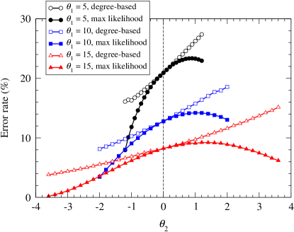
Figure 2: The fraction of nodes classified incorrectly in tests on stochastic block model networks parametrized according to Eq. (33), as a function of $\theta_{2}$ for fixed $r=2$ and three different values of $\theta_{1}$ as indicated. Solid points represent results for the maximum likelihood method described in this paper. Open points are the results of a simple division according to vertex degree. Each point is an average over 10 networks of a million nodes. Statistical errors are smaller than the data points. The parameter ranges are different for different curves because they are constrained by the requirement that edge probabilities be nonnegative and that $c_{11}>c_{12}>c_{22}$, which means that $\theta_{2}$ must satisfy $-\theta_{1}/r<\theta_{2}<\theta_{1}(1-1/r)/(r+1)$.

It is fair to say, however, that the error rates of the two algorithms are comparable in some cases and the naive algorithm does moderately well under the right conditions, with error rates of around 10 or 20 percent for many choices of parameter values. There are a couple of possible morals one can derive from this observation. On the one hand, if one is not greatly concerned with accuracy and just wants a quick-and-dirty division into core and periphery, then dividing vertices by degree may be a viable strategy. The belief propagation method usually does better, but it is also more work to program and requires more CPU time to execute. For some applications we may feel that the additional effort is not worth the payoff. Moreover, since the belief propagation method is optimal in the sense discussed earlier, we know that, at least for the definition of core–periphery structure used here, no other algorithm will out-perform it, so the loss of accuracy seen in Fig. 2 is the largest such loss we will ever incur when using the degree-based algorithm. In other words, this is as bad as it gets, and it’s not that bad.

On the other hand, as we have said, one does not in most cases know the sizes of the groups into which the network is to be divided, in which case one must use the EM algorithm even for a degree-based division. The computations involved, which are described in Section IV.1, are less arduous than those for the full belief propagation algorithm but significantly more complex than a simple division by degree only, and this eliminates some of the advantages of the degree-based approach.

Furthermore, while the number of nodes on which our method and the degree-based algorithm differ is sometimes quite small, it may be these very nodes that are of greatest interest. It’s true that it is typically the higher-degree nodes that fall in the core and the lower-degree ones that fall in the periphery. But when the two algorithms differ in their predictions it is precisely because some of the low-degree nodes correctly belong in the core or some of the high-degree ones in the periphery, which could lead us to ask what is special about these nodes. Who are the people in a social network, for example, who fall in the core even though they don’t have many connections? Who are the well-connected people who fall in the periphery? These people may be of particular interest to us, but they can only be identified by using the full maximum likelihood algorithm. The degree-based algorithm will, by definition, never find these anomalous nodes.

V.2 Real-world examples

Figure 3 shows an application of our method to a real-world network, the Internet, represented at the level of autonomous systems. This network is expected to have clear core–periphery structure: its general structure consists of a large number of leaves or edge nodes—typically client autonomous systems corresponding to end users like ISPs, corporations, or educational institutions—plus a smaller number of well-connected backbone nodes Pastor-Satorras and Vespignani (2004); Holme (2005). This structure is reflected in the decomposition discovered by our analysis, indicated by the blue (core) and yellow (periphery) nodes in the figure. The bulk of the nodes are placed in the periphery, while a small fraction of central hubs are placed in the core. Note, however, that, as discussed earlier, the algorithm does not simply divide the nodes according to degree. There are a significant number of high-degree nodes that are placed by the algorithm in the periphery because of their position on the fringes of the network, even though their degree might naively suggest that they be placed in the core.

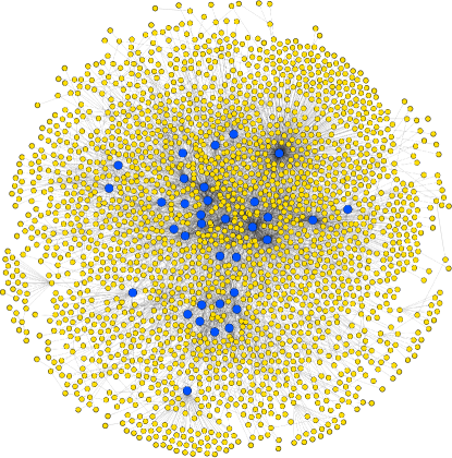
Figure 3: Core–periphery division of a 1470-node representation of the Internet at the level of autonomous systems Pastor-Satorras et al. (2001). Nodes placed in the core by our analysis are drawn larger and in blue; nodes in the periphery are smaller and in yellow. The network was constructed from data from the Oregon Routeviews Project and represents an older snapshot, chosen for the network’s relatively small size. Our methods can easily be applied to larger networks, but smaller size makes the visualization of the results clearer.

Figure 4 shows a contrasting example. The network in this figure, drawn from a 2005 study by Adamic and Glance Adamic and Glance (2005) is a web network, representing a set of 1225 weblogs, personal commentary web sites, devoted in this case to commentary on US politics. Edges represent hyperlinks between blogs, which we treat as undirected for the purposes of our analysis. This network has been studied previously as an example of community structure, since it displays a marked division into groups of conservative and liberal blogs. The figure is drawn so as to make these groups clear to the eye—they correspond roughly to the left and right halves of the picture—and the core–periphery division is indicated once more by the blue (core) and yellow (periphery) nodes.

As the figure shows, the analysis finds a clear separation between core and periphery, and moreover finds a separate core in each of the two communities. In effect, the conservative blogs are divided into a conservative core and periphery, and similarly for the liberal ones. A direct examination of the list of core nodes in each community finds them to contain, as we might expect, many prominent blogs on either side of the aisle, such as the National Review and Red State on the conservative side and Daily Kos and Talking Points Memo on the liberal side.

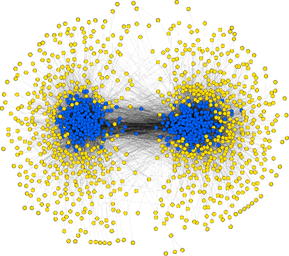
Figure 4: Core–periphery division of a network of hyperlinks between political blogs taken from Adamic and Glance (2005). The network naturally separates into conservative and liberal communities, clearly visible as the two clusters in this picture. Within each group our algorithm finds a separate core and periphery indicated by the blue and yellow nodes respectively.

VI Conclusion

We have examined core–periphery structure in undirected networks, proposing a first-principles algorithm for identifying such structure by fitting a stochastic block model to observed network data using a maximum likelihood method. The maximization is implemented using a combination of an expectation–maximization algorithm and belief propagation. The algorithm gives good results on test networks and is efficient enough to scale to networks of a million nodes or more. By a linearization of the belief propagation equations we are also able to show the method to be immune from the detectability threshold seen in the application of similar methods to community detection. In the community detection case the algorithm (and indeed all algorithms) fail when community structure in the network is too weak, but there is no such failure for the core–periphery case. Core–periphery structure is always detectable, no matter how weak it is.