Practical Topological Cluster State Quantum Computing Requires Loss Below 1%

Abstract

The surface code cannot be used when qubits vanish during computation; instead, a variant known as the topological cluster state is necessary. It has a gate error threshold of $0.75\%$ and only requires nearest-neighbor interactions on a 2D array of qubits. Previous work on loss tolerance using this code only considered qubits vanishing during measurement (Barrett and Stace, 2010). We begin by also including qubit loss during two-qubit gates and initialization, and then additionally consider interaction errors that occur when neighbors attempt to entangle with a qubit that isn’t there. In doing so, we show that even our best case scenario requires a loss rate below $1\%$ in order to avoid considerable space-time overhead.

I Introduction

Quantum error correction (QEC) codes have made it plausible to perform arbitrarily robust quantum computation using imperfect hardware. Each gate must be below a threshold error rate, which is unique to the code and types of error present. At $\sim$$1\%$ (Fowler et al., 2012a), the surface code (Bravyi and Kitaev, 1998) has the highest threshold of any code needing only a 2D array of qubits with nearest-neighbor interactions – the most practical experimental requirements of any code with a similar threshold.

Quantum hardware based on linear optics (Fortescue et al., 2014), optical lattices (Vala et al., 2005), and trapped-ions (Blakestad et al., 2011; Wright et al., 2013) suffers from qubit loss. Qubit loss – or simply loss – is defined as when a qubit vanishes during computation, but can be detected and replaced at measurement. This differs from manufacturing faults, where a qubit is permanently unusable, requiring alternate methods to work around. Loss is also different to leakage, where a qubit transitions into a non-computational state rather than disappearing entirely.

Unfortunately, the surface code cannot be used when loss can occur, regardless of how unlikely. The presence of these errors necessitates the use of another code, the topological cluster state (Raussendorf et al., 2003). While the topological cluster state is a 3D code, it can be implemented on a 2D lattice with nearest neighbor interactions, just as with the surface code. It therefore has the same physical requirements – with a threshold of $\sim$$0.75\%$ (Fowler et al., 2012b) – but can also continue to correct errors when some qubits vanish.

Initial work to determine how much loss is tolerable using the topological cluster state was promising – indicating that the loss threshold was $\sim$$24.9\%$ (Barrett and Stace, 2010). This threshold is true under a model where loss occurs only during measurement. However, of the hardware implementations where loss can occur, the qubits can become lost at any time rather than only during measurement (Wright et al., 2013; Knill et al., 2000; Mandel et al., 2003; Olmschenk et al., 2010).

There has been limited analysis of what errors occur when two qubits are intended to be interacted but one of the pair is missing (Herrera-Marti et al., 2010). When a two-qubit entangling gate is used, but one of the pair has vanished, it is unclear what occurs to the remaining qubit. Depending on the implementation of the hardware, the qubits neighboring a lost one may acquire additional errors during two-qubit interactions.

The results presented here are based on current experimental targets for computational error, $p\in\{10^{-3},10^{-4}\}$. While the thresholds under our models are greater than $1\%$, we consider the amount of loss to be practical only if a quantum computer would require fewer than twice as many qubits when compared to one without any loss at all. Further details are provided in the Results (Sec. X).

To make this paper self contained, background information has been included covering stabilizers in Sec. II, cluster states in Sec. III, the topological cluster state in Sec. IV, error correction in Sec. V, and how loss is handled in Sec. VI. Those familiar with the topological cluster state are invited to skip to Sec. VII where we describe the models for loss we have used. Sec. VIII outlines how we have calculated overhead. Sec. IX discusses how the simulations were performed, Sec. X includes our results, and Sec. XI the discussion.

II Stabilizers

The stabilizer (Gottesman, 1997) of a state $\ket{ψ}$ is the group $\mathcal{G}$ of operators $A_{i}$, called stabilizers, that act on $\ket{ψ}$ without modifying it.

$$A_{i}\ket{ψ}=\ket{ψ}$$

Without the presence of errors, we know our state $\ket{ψ}$ is in the simultaneous $+1$ eigenstate of the stabilizers. This, as will be explained, allows a generating set for the group $\mathcal{G}$ of stabilizers to be used to represent the state. For example, the $\hat{Z}$ operator is a stabilizer for the state $\ket{0}$ and a generator of its stabilizer group. This implies that if we know that our state is stabilized by the $\hat{Z}$ operator, then our state is the $+1$ eigenstate of $\hat{Z}$, namely $\ket{0}$. We will only work with stabilizers that are tensor products of the $\hat{X}$ (bit flip), $\hat{Z}$ (phase flip), $\hat{Y}$ (bit and phase flip) and $\hat{I}$ (identity) operators.

In what is a somewhat confusing use of terminology, the stabilizers of a state $\ket{ψ}$ often refers instead to $\mathcal{S}$, a generating set of $\mathcal{G}$. This stabilizer generator set will typically have $n$ elements, where $n$ is the number of qubits in the state $\ket{ψ}$.

In line with this, a stablizer of the state $\ket{ψ}$ often refers to an element $A$ of the stabilizer generator, $\mathcal{S}$ ($A\in\mathcal{S}$). By definition, the element $A$ is also an element of $\mathcal{G}$ ($A\in\mathcal{G}$). This terminology is the result of more commonly working with the generating set $\mathcal{S}$ and the elements of $\mathcal{S}$ rather than with the entire group.

There are many subsets of $\mathcal{G}$ that form a valid generating set. Due to the closure of the group $\mathcal{G}$, any valid generating set $\mathcal{S}$ can be transformed into another generating set $\mathcal{S}^{\prime}$ by repeatedly taking the matrix product of elements of $\mathcal{S}$ and replacing one of these elements with the result. Henceforth, the one chosen is the most convenient set to work with.

Stabilizers are of interest because they allow us to represent some complex entangled states without having to write the actual state. The stabilizer formalism cannot be used to express all quantum states, but it is sufficient when defining the topological cluster state. In order to see how we can represent a state $\ket{ψ}$ by its stabilizers, we first need to see how the stabilizing set evolves when a unitary operator $U$ is applied.

$$A\ket{ψ} =\ket{ψ}$$ (1)

$$UA\ket{ψ} =U\ket{ψ}$$ (2)

$$UAU^{\textdagger}U\ket{ψ} =UU^{\textdagger}U\ket{ψ}$$ (3)

$$(UAU^{\textdagger})U\ket{ψ} =U\ket{ψ}$$ (4)

As $U$ is unitary, $U^{\textdagger}U$ is equal to the identity operator, and hence can be introduced without modifying the equation. The result of this shows that if $A$ stabilizes $\ket{ψ}$, then $UAU^{\textdagger}$ stabilizes $U\ket{ψ}$. Therefore, rather than looking at how the state $\ket{ψ}$ evolves, we can instead find a stabilizing set for $\ket{ψ}$ and track how the stabilizers evolve (Aaronson and Gottesman, 2004; Anders and Briegel, 2006).

Consequently, we can represent a state using $n$ stabilizers, each of $n$ operators, requiring only $n^{2}$ memory to store the state $\ket{ψ}$. This is superior to potentially having to store the amplitudes for $2^{n}$ states if one was to track the evolution of $\ket{ψ}$ itself.

The most basic examples of stabilizers are the $\hat{X}$ operator on the $\ket{+}$ state, $\hat{X}\ket{+}=\ket{+}$, and $\hat{Z}$ operator on the $\ket{0}$ state, $\hat{Z}\ket{0}=\ket{0}$. A basic 2 qubit example is the state $\frac{\ket{00}+\ket{11}}{\sqrt{2}}$ that can be represented by the stabilizers:

$A_{1}$	$X_{1}$	$\otimes$	$X_{2}$
$A_{2}$	$Z_{1}$	$\otimes$	$Z_{2}$

III Cluster States

A cluster state is any where each qubit is initialized in the $\ket{+}$ state, and then at least one $C_{Z}$ gate performed. We will use the stabilizer formalism to describe our cluster states. There is a convenient way to determine a set of generators for a given cluster state $\ket{ψ}$:

$$A_{i}=X_{i}\otimes_{q_{j}\in\text{nghb}(q_{i})}Z_{j},$$

where $i$ indexes a qubit in the state $\ket{ψ}$ and $\text{nghb}(q_{i})$ is the set of qubits connected to $q_{i}$ via $C_{Z}$ gates.

Consider the 2D cluster state in Fig. 1. Each qubit is initialized to the $\ket{+}$ state, which is stabilized by $\hat{X}$. Since each qubit is currently independent, we can stabilize the 5-qubit state $\ket{ψ}=\ket{+}_{1}\ket{+}_{2}\ket{+}_{3}\ket{+}_{4}\ket{+}_{5}$ with the following stabilizers:

Figure 1: The 5 qubit cluster state found on each of the faces of a 3D topological cluster state cell (Fig. 2). Black dots are the qubits $q_{1}$ to $q_{5}$, initialized in the $\ket{+}$ state. Black lines indicate $C_{Z}$ gates between the two connected qubits.

$A_{1}$	$X_{1}$	$\otimes$	$I_{2}$	$\otimes$	$I_{3}$	$\otimes$	$I_{4}$	$\otimes$	$I_{5}$
$A_{2}$	$I_{1}$	$\otimes$	$X_{2}$	$\otimes$	$I_{3}$	$\otimes$	$I_{4}$	$\otimes$	$I_{5}$
$A_{3}$	$I_{1}$	$\otimes$	$I_{2}$	$\otimes$	$X_{3}$	$\otimes$	$I_{4}$	$\otimes$	$I_{5}$
$A_{4}$	$I_{1}$	$\otimes$	$I_{2}$	$\otimes$	$I_{3}$	$\otimes$	$X_{4}$	$\otimes$	$I_{5}$
$A_{5}$	$I_{1}$	$\otimes$	$I_{2}$	$\otimes$	$I_{3}$	$\otimes$	$I_{4}$	$\otimes$	$X_{5}$

Then, we can see how the application of $C_{Z}$ affects the stabilizers on two qubits:

$$C_{Z} =C_{Z}^{\dagger}$$ (5)

$$C_{Z}(I\otimes X)C_{Z} =Z\otimes X$$ (6)

$$C_{Z}(X\otimes I)C_{Z} =X\otimes Z$$ (7)

$$C_{Z}(I\otimes Z)C_{Z} =I\otimes Z$$ (8)

$$C_{Z}(Z\otimes I)C_{Z} =Z\otimes I$$ (9)

Following the $C_{Z}$ interactions outlined in Fig. 1, we want to take the stabilizers from state $\ket{ψ}$ and update them to stabilize the state $\ket{ψ^{\prime}}=\Lambda_{1,3}\Lambda_{2,3}\Lambda_{4,3}\Lambda_{5,3}\ket{ψ}$ where $\Lambda_{i,j}$ is a $C_{Z}$ applied between qubits $q_{i}$ and $q_{j}$. Based on the definition of stabilizers, we know that if $A$ is a stabilizer of $\ket{ψ}$, then $UAU^{\dagger}$ stabilizes $U\ket{ψ}$. Therefore, $\Lambda_{1,3}A\Lambda_{1,3}^{\dagger}$ stabilizes $\Lambda_{1,3}\ket{ψ}$. Repeating this for each of the $C_{Z}$ gates results in the following set of stabilizers:

$A_{1}$	$X_{1}$	$\otimes$	$I_{2}$	$\otimes$	$Z_{3}$	$\otimes$	$I_{4}$	$\otimes$	$I_{5}$
$A_{2}$	$I_{1}$	$\otimes$	$X_{2}$	$\otimes$	$Z_{3}$	$\otimes$	$I_{4}$	$\otimes$	$I_{5}$
$A_{3}$	$Z_{1}$	$\otimes$	$Z_{2}$	$\otimes$	$X_{3}$	$\otimes$	$Z_{4}$	$\otimes$	$Z_{5}$
$A_{4}$	$I_{1}$	$\otimes$	$I_{2}$	$\otimes$	$Z_{3}$	$\otimes$	$X_{4}$	$\otimes$	$I_{5}$
$A_{5}$	$I_{1}$	$\otimes$	$I_{2}$	$\otimes$	$Z_{3}$	$\otimes$	$I_{4}$	$\otimes$	$X_{5}$

Henceforth the tensor product symbol will be omitted for brevity.

IV Topological Cluster State

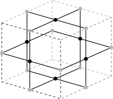
Figure 2: A Topological Cell State. The black and gray dots indicate qubits initialized in the $\ket{+}$ state, while solid lines indicate the application of a $C_{Z}$ gate. The black dots at the center of the faces are measured in the $\hat{X}$ basis ($M_{X}$) and form the measurement product of the cell. The dotted lines are a visual aid only.

The topological cluster state is composed of a 3D tiling of cells, illustrated in Fig. 2. Despite being a 3D tiling, the state can be implemented on a 2D architecture with only nearest-neighbor interactions (Fig. 7). A single cell touches 18 qubits, each prepared in the $\ket{+}$ state, with $C_{Z}$ gates applied from each face qubit to each neighboring edge qubit. In this configuration, there exists a stabilizer consisting of only $\hat{X}$ measurements on the qubits at the center of each face. When tiled in 3D, each face qubit is shared with its neighbor, while each edge qubit is shared by a total of four cells. Those unfamiliar with stabilizers and matrix products may find an explicit derivation of the cell state aids their understanding (Appendix. A).

When measuring the six face qubits in the $\hat{X}$ basis, each will either be in the $+1$ or $-1$ eigenstate of $\hat{X}$. Due to the structure of the cell, with no errors present, the cell will be in the $+1$ eigenstate of the six face qubits. A $\hat{Z}$ error on one of the face qubits will flip the eigenstate measured, causing the product of the six face measurements, called the measurement product, to become $-1$. Cells where an odd number of errors have occurred can be identified by their $-1$ measurement products, referred to as detection events. As each face qubit is shared by a neighbor, the location of errors can be inferred by the pattern of detection events. If two neighboring cells are both measured to be in the $-1$ eigenstate of the six face qubits, then it is likely that the qubit on the face shared by the two neighbors has become erroneous (Fig. 3).

The topological cluster state only corrects $\hat{Z}$ and $M_{X}$ errors. This is sufficient as $\hat{X}$ errors have no effect; an $\hat{X}$ error occurring just before measurement does not change the measurement outcome, while one occurring earlier will cause $\hat{Z}$ errors on one or more neighboring qubits (Eqs. 6 – 9). Since each cell is stabilized by only $\hat{X}$ basis measurements, we can ignore the $\hat{X}$ errors as long as we correct the resultant $\hat{Z}$ errors (Fowler and Goyal, 2009).

The full set of qubits tiled in both space and time is called a lattice. There exists a second lattice offset by one in both space dimensions and in time, where each face qubit of the first lattice becomes an edge qubit in the second, as well as the reverse. We arbitrarily call one the primal lattice and the other the dual lattice. This allows for complete error correction despite a single cell only detecting errors on the face qubits; the eight dual cells that encompass a primal cell will have the edge qubits as face qubits. An error is therefore classified as either primal or dual depending on which lattice it is detected in. These two interwoven lattices are also necessary for the implementation of two-qubit logical gates (Fowler and Goyal, 2009).

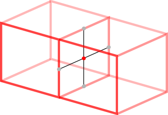
Figure 3: Detecting the location of an error using adjacent cells. The dark (red) dot is the qubit that has suffered an error. The face stabilizer shared by the cells has been shown, the others have been omitted for clarity. Each face qubit is shared by two adjacent cells. The thick lines indicate the boundaries of cells where a detection event occurs. The error causes a detection event to occur in both cells, allowing the location of the error to be inferred.

The inference of errors from detection events is unfortunately inexact. Multiple patterns of errors can create the same pattern of detection events due to an even number of errors being undetectable to a cell. An even number of errors will result in an even number of $-1$ measurements, leaving the cell in the $+1$ eigenstate of the faces. Fig. 4 shows a chain of three errors, where only the cells at either end have a $-1$ measurement product (and hence a detection event).

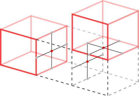
Figure 4: A chain of three errors, in space and time, affecting four cells. This demonstrates how chains can occur through multiple axes. The dark (red) dots indicate qubits where an error has occurred. Thick solid lines indicate the boundary of a cell where a detection event occurs. Thin dotted lines indicate the boundary of a cell where no detection event occurs.

The calculation of detection events and the inference of errors will be done by classical hardware running in parallel with a quantum computer (Fowler et al., 2012a). Given the observed pattern of detection events, Edmonds’ minimum weight perfect matching algorithm (Edmonds, 1965) can be used determine where errors are likely to have occurred. As the rate of error increases, error combinations leading to the same detection events become more frequent and incorrect inference becomes more common. It has been shown that this algorithm can be parallelized to $\text{O}(1)$ given fixed computing resources per unit area (Fowler, 2013a), an essential property if the classical software is to scale with the size of a large quantum computer. A number of other methods are being studied in an attempt to get better performance during inference (Duclos-Cianci and Poulin, 2010, 2014; Wootton and Loss, 2012; Hutter et al., 2014; Bombin et al., 2012; Bravyi et al., 2014).

Logical qubits are formed in the topological cluster state by creating defects, where regions of the cluster state have their face stabilizers measured in the $\hat{Z}$ basis. How logical qubits are formed and manipulated to perform computation is unnecessary to understand the results presented. We refer the reader to (Fowler and Goyal, 2009) for an overview, and to the references (Raussendorf et al., 2003; Raussendorf and Harrington, 2007; Raussendorf et al., 2007) for more details.

V Error Correction

The distance $d$ of the code is the minimum number of physical qubits that need to be manipulated in order to connect two defects or encircle a defect. If a chain of errors joins two defects of the same type (primal to primal, or dual to dual), a logical error occurs.

A logical error also occurs if a defect is connected to a boundary, or if two boundaries of the same type are connected. A boundary is the smooth edge of the lattice which ends in complete cells. In our chosen assignment of primal and dual, the primal boundaries are at the top and bottom of the lattice with the dual boundaries at the left and right (Fig 5).

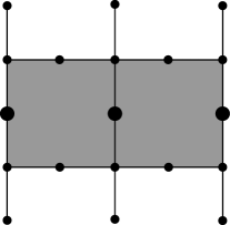
Figure 5: A single layer of a distance $3$ topological cluster state. Black dots indicate qubits, black lines indicate $C_{Z}$ gates. Gates between this layer and others are omitted for clarity. The gray squares are a visual indicator for the two complete dual cells. Dual boundaries are located to the left and right. The larger black dots are the three qubits where a chain of errors could connect the two dual boundaries. A second layer which is identical, except rotated 90 degrees, would have primal cells in gray and boundaries at the top and bottom.

Due to the inference in error correction, a logical error can occur with fewer than $d$ errors. The minimum number of errors that can cause a logical error is $d_{e}$:

$$d_{e}=\bigg{\lfloor}\frac{d+1}{2}\bigg{\rfloor}$$

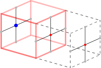
Figure 6: Two cells illustrating a distance $3$ fragment of a larger topological cluster state. The two ($d_{e}$) smaller dark dots are qubits with errors. The thick solid lines indicate the boundary of a cell with a detection event. The larger dark dot indicates the most likely error pattern that would create the observed detection event. By applying a correction at the larger dark qubit, where one isn’t needed, a chain spans the lattice resulting in a logical error.

Take the example of $d=3$ as seen in Fig. 6; $d_{e}$ in this instance is $2$. A line of $3$ qubits crosses the two cells. A single error from one end has the same detection event pattern as two errors in a row from the opposite end. Therefore, when the two error case occurs with probability $O(p^{d_{e}})$ the minimum weight perfect matching algorithm will infer the single error case. By applying an erroneous correction, the algorithm introduces another error completing the chain and connecting one edge of the lattice to the other, forming a logical error.

For each set of errors that occupies at least $d_{e}$ positions along an axis, there exists another set with equal or greater probability that will typically be chosen by minimum weight matching, resulting in a logical error. In should be emphasized that while the probability of a logical error $p_{L}$ is proportional to $p^{d_{e}}$, the occurrence of $d_{e}$ errors does not always result in a logical error.

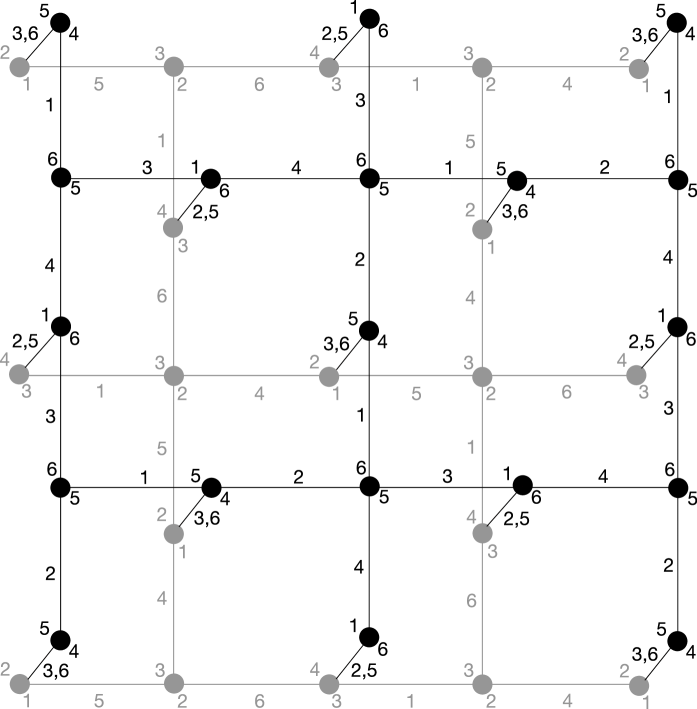
Figure 7: A distance $3$ topological cluster state on a 2D array of qubits. Each line is a $C_{Z}$ gate and is labelled to indicate in which timestep(s) the gate is applied. The black dots indicate qubits. The number to the top left of a qubit indicates the timestep the qubit is initialized in, the number to the bottom right when it is measured. Dark and light provide visual separation between the two layers. When implemented on a 2D architecture, no such distiniction exists, and the qubits are laid out physically as presented.

By noting that each qubit is only interacted with its four neighbors, it is possible to implement a 3D cell in only two layers (Fig. 7). With careful timing of the $C_{Z}$ gates, each qubit that needs to interact in the arbitrarily assigned up direction can be initialized then interacted with its down neighbor. This neighbor will have then completed all four of its interactions, allowing it to be measured and reinitialized. This new qubit can then be interacted with the original qubit becoming its up neighbor as well. This can be further implemented on a strictly 2D physical architecture by interweaving the two layers into a single physical layer.

VI Handling Qubit Loss

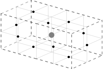
Figure 8: Two adjacent cells with a shared face qubit that has been lost. The dotted dark gray lines indicate the boundary of the merged stabilizer. The black dots indicate the ten qubits whose measurements will form the measurement product for the merged stabilizer. The large gray dot indicates the lost qubit.

Lost qubits break the method of detecting errors outlined in Section IV. Consider again the case of two cells sharing a qubit that has suffered an error (Fig. 3), however instead of an $\hat{X}$, $\hat{Y}$, or $\hat{Z}$ error, the qubit was lost entirely. In this case, the lost qubit cannot be measured, and neither cell would have six measurement results. Given that both cells should be in the $+1$ eigenstate of all six measurement results, the measurement products are meaningless without the last.

To allow for loss, we take advantage of the product of two stabilizers also being a stabilizer. The product of two cell stabilizers forms a new stabilizer consisting of the remaining ten face qubits, and is independent of the shared qubit (Fig. 8). We cannot correct the loss error, however this process can yield a valid detection event with which to detect errors on the remaining qubits (Fig. 9). Connected sets of loss errors repeat this process creating larger and larger stabilizers. The merging of stabilizers effectively reduces the number of computational errors that can be tolerated. This highlights the importance of the topological cluster state, as its short error correction cycle followed by measuring and replacing all qubits puts a limit on how long the reduced distance is in effect.

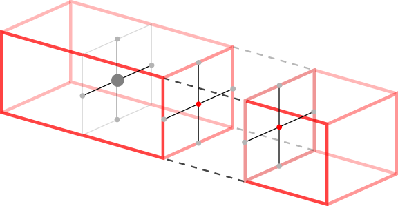
Figure 9: An error chain including a lost qubit error. The thick solid lines indicate cells where a detection event occurs. Small dark dots indicate errors. The large gray dot indicates the lost qubit. Note that the merged stabilizer due to the lost qubit behaves like a regular cell, with the detection events occurring at both ends of the regular error chain.

VII Modeling Loss

Each qubit in the topological cluster state undergoes the same gate sequence, albeit staggered in time. This sequence includes initialization, measurement, identity (storage), Hadamard, and controlled-Z ($C_{Z}$).

In our models, and those we compare to, each gate introduces computational errors with equal probability, $p_{comp}$. These errors manifest as unintended $\hat{I}$, $\hat{X}$, $\hat{Y}$, or $\hat{Z}$ operations on the involved qubit(s), each with an equal chance of occurring. This model of computational error is identical to that published previously (Fowler et al., 2012b).

Previous generic analysis of the topological cluster state and its tolerance to loss only considered the performance when qubits were lost during measurement (Barrett and Stace, 2010), though a hardware-specific analysis has considered loss occurring during both initialization and measurement (Herrera-Marti et al., 2010).

For our analysis loss is assumed to be detectable only at measurement and occurs with equal probability $p_{loss}$ on all gates, except Hadamard, where we assume there are no loss events. Single qubit Hadamard gates are typically much simpler and faster than other gates, contributing negligible loss. With ion trap quantum hardware, ion movement and traversing junctions are now well-controlled, introducing very little additional loss over baseline background gas collisions. Since such collisions can occur at any time, loss can occur during any gate, making loss less frequent during faster gates (Wright et al., 2013).

When considering linear optical hardware, deterministic generation and measurement of photons is extremely difficult, while two-qubit gates are challenging as they require photon memory and feedforward processing. These processes are therefore associated with significant photon loss. By contrast, single-qubit gates require a simple beam splitter, with negligible loss (Knill et al., 2000). This assumption holds true for optical lattice hardware as well, where the single qubit rotation of the Hadamard gate is much faster than the other gates (Mandel et al., 2003; Olmschenk et al., 2010).

In our models, loss events can occur after initialization, after each $C_{Z}$ gate and during measurement (Fig. 10). This results in an average of $6p_{loss}$ loss events per qubit, per round of error correction. This is six times more than a model considering only loss during measurement.

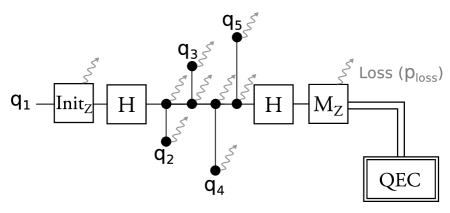
Figure 10: A round of error correction for a single qubit using the topological cluster state, with loss occurring at initialization, two-qubit gates, and measurement. The qubit $q_{1}$ is initialized in the $\hat{X}$ basis, interacted with its four neighbors using $C_{Z}$ gates, and then measured. The measurement result is passed to a classical computer for error correction. The gray arrows indicate where a qubit may be lost with probability $p_{loss}$.

The second of our two error models also introduces loss interaction errors, which occur with probability $p_{lint}$. A two-qubit gate, such as the $C_{Z}$ gate, assumes the interaction between two present qubits. If one of the two qubits is missing, the gate may fail and introduce error on the remaining qubit (Fig. 11), we which refer to as a loss interaction error. We choose $p_{lint}=1$, such that any qubit being interacted with a lost qubit will always acquire an $\hat{I}$, $\hat{X}$, $\hat{Y}$, or $\hat{Z}$ error, upper bounding the behaviour. Some hardware implementations may be able to reduce, or entirely avoid this error by constructing a gate that can only work in the presence of two qubits.

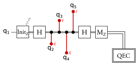
Figure 11: Demonstration of the effect of loss interaction errors. The grey arrow indicates where the qubit is lost. The thick grey line indicates the time line of the lost qubit through the circuit. With $p_{lint}=1$, each neighbor ($q_{2}$, $q_{3}$, $q_{4}$, $q_{5}$) acquires an $\hat{I}$, $\hat{X}$, $\hat{Y}$, or $\hat{Z}$ error. In this instance $q_{2}$ and $q_{4}$ acquire an $\hat{X}$ error, $q_{3}$ acquires $\hat{Y}$ and $q_{5}$ acquires $\hat{I}$.

VIII Measuring Overhead

In order to calculate the overhead of loss we define a volume of space-time known as a plumbing piece. Consider a square defect of circumference $d$. Such a defect must be distance $d$ from all other defects in space and time. A space-time volume containing this defect, and all necessary space around it (see Fig. 12) is a plumbing piece and will have an edge length (in cells) of:

$$n\approx\frac{5d}{4}$$

Each cell touches 18 qubits. Given that each face qubit is shared by its neighbor, and each edge qubit is shared with three other neighbors, a single cell is effectively six qubits. The total plumbing piece volume in qubits is:

$$V \approx 6\left(\frac{5d}{4}\right)^{3}$$ (10)

We can decompose this into physical and time qubits as follows. Each cell requires two layers of $3n^{2}$ physical qubits, while the $n$ cells in time results in a total of $6n^{3}$.

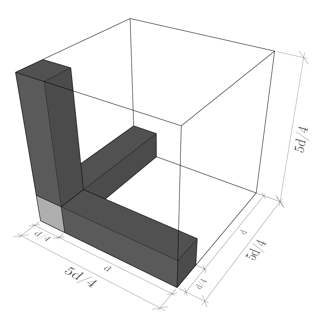
Figure 12: A plumbing piece with volume $(5d/4)^{3}$. This defect example contains a cubic fragment (light gray) of circumference $d$ (edge length $d/4$) and with prisms of length $d$ separating it from all neighbors (dark gray).

Plumbing piece volume is measured in units of qubit-rounds. This takes into account not only the physical resource overhead, but the additional time (in rounds of error correction) necessary to implement larger distances. Focusing on a single plumbing piece provides a measure of overhead independent of any specific algorithm. This allows relative performance comparisons regardless of future improvements to algorithms and circuit compression.

IX Simulation

Simulations were performed using an updated version of our Autotune software (Fowler et al., 2012b). The logical error rate ($p_{L}$) of a given error model is determined by a continuous simulation of an ever growing topological cluster state. Each iteration of the simulation extends the problem by $t_{check}$ rounds. The problem is then capped by simulating two more rounds, with all errors disabled, to ensure that all cells have been completed. The detection events are then analysed to determine if a logical error has occurred. Finally, the actions taken to cap the problem are reversed in order to continue the simulation of the next $t_{check}$ rounds.

In more detail, each iteration begins with the simulation of $t_{check}$ rounds of the topological cluster state. This is followed by all errors being disabled and two more rounds of error correction being performed to finalize any remaining cells. The value of $t_{check}$ is dependent on the expected $p_{L}$, starting at $1$ when $p_{L}$ is expected to be high (large $p_{comp}$ and $p_{loss}$) and up to $10^{4}$ when $p_{L}$ is expected to be low (small $p_{comp}$ and $p_{loss}$).

We then use the Blossom V (Kolmogorov, 2009) matching library in order to match the detection events. Autotune was updated to make use of this publicly available library to make it both more useful to other researchers, and to make our results more readily reproducible. This comes with the downside of being slower than our previous matching library (Fowler et al., 2012c).

The Autotune software generates weights for the matching problem by analyzing the user provided arbitrary stochastic error model to determine where and when every possible error is detected. Many different errors can lead to the same pair of detection events, and the total probability of all such errors can be converted to a useful weight by taking the negative log. These weights are stored in a 3-D graph structure, so that they can be used throughout the simulation. By merging the weights of the underlying lattice when qubits are lost, the matching can accurately account for these errors.

After matching we can determine if a logical error has occurred by observing if there has been a change in the number of errors along a boundary. Finally, the two perfect rounds of error correction are undone and allowing the simulation of another $t_{check}$ rounds.

In order to manage the problem size and memory use, detection events and associated data are removed after $t_{delete}$ rounds have occurred. This is possible due to it becoming highly unlikely that a detection event sufficiently far in the past needs to be rematched. The value of $t_{delete}$ was chosen to be $5d$.

The simulations were performed in this manner as it most closely resembles the operation of an actual quantum computer. They were designed so that it was feasible to replace the input error model with one generated from experiment (Fowler et al., 2014), and use experimental measurement results as opposed to simulating them.

X Results

For the model including initialization, two-qubit and measurement loss errors, we dynamically generated graphs plotting the probability of logical error ($P_{L}$) against the probability of loss ($p_{loss}$). We generated these graphs for three fixed amounts of computational error: $p_{comp}=0$ to determine the behavior of loss alone; and $p_{comp}\in\{10^{-3},10^{-4}\}$ to determine the behavior of loss at two current experimental targets for computational error. Under this error model we observe a threshold loss error rate of $\sim$$2$–$5\%$.

With computational error of $0.1\%$ ($p_{comp}=10^{-3}$) (Fig. 13), the effect of loss is negligible when the rate of loss is less than $0.01\%$ ($p_{loss}=10^{-4}$). The curves asymptote to the behavior obtained when only computational error is considered ($p_{loss}=0$), as expected (Fowler et al., 2012b).

We verify the correct behavior of our loss implementation by observing that with no computational error ($p_{comp}=0$) (Fig. 15), the curves asymptote toward functions defined by the minimum number of errors that can lead to a logical failure, $d-1$. With no computational error, the only form of logical error is when a stabilizer has been merged to the point of bordering both boundaries of the same type, then needs to be merged with the boundary. That is, at sufficiently low $p_{loss}$ the logical error rate can be approximated by:

$$P_{L}\approx cp_{loss}^{d-1}$$ (11)

For the model where loss interaction errors are also included ($p_{lint}=1$), we observe an order of magnitude drop in the threshold error rate to $\sim$$0.2$–$0.5\%$. With high computational error ($p_{comp}=10^{-3}$) (Fig. 16) we observe that the impact of loss becomes negligible when the rate of loss is an order of magnitude lower than the model with no interaction errors ($p_{loss}=10^{-5}$).

A single loss event can form a chain of two computational errors when loss interaction errors occur. This allows one loss error to act as two errors, reducing the minimum number of errors required to cause a logical error to $\big{\lfloor}\frac{d+3}{4}\big{\rfloor}$, adjusting the asymptotics as observed (Fig. 18).

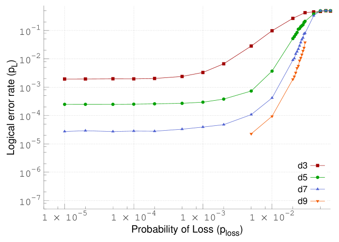
Figure 13: Logical error rate ($P_{L}$) vs. Probability of loss ($p_{loss}$). Fixed computational error ($p_{comp}=10^{-3}$) and no loss interaction error ($p_{lint}=0$).

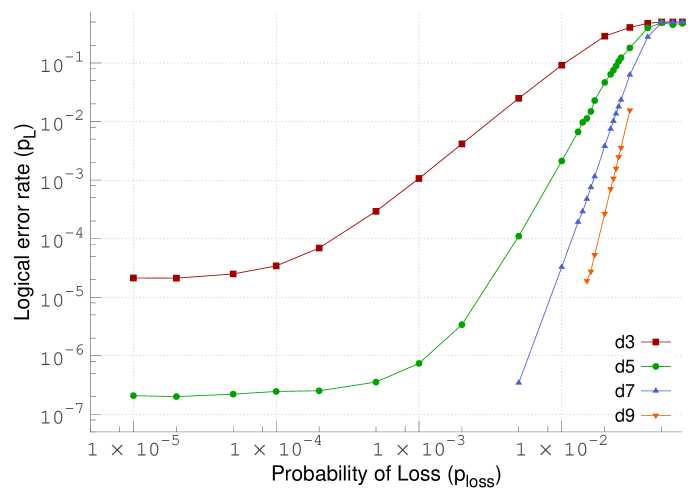
Figure 14: Logical error rate ($P_{L}$) vs. Probability of loss ($p_{loss}$). Fixed computational error ($p_{comp}=10^{-4}$) and no loss interaction error ($p_{lint}=0$).

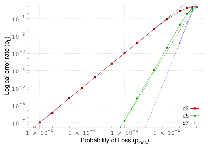
Figure 15: Logical error rate ($P_{L}$) vs. Probability of loss ($p_{loss}$). Fixed computational error ($p_{comp}=0$) and no loss interaction error ($p_{lint}=0$). Dotted lines indicate asymptotic lines where logical errors predominantly caused by the minimum necessary ($\approx cp_{loss}^{d-1}$).

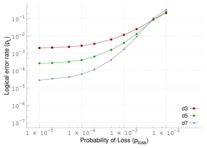
Figure 16: Logical error rate ($P_{L}$) vs. Probability of loss ($p_{loss}$). Fixed computational error ($p_{comp}=10^{-3}$) and 100% chance of loss interaction error ($p_{lint}=1$).

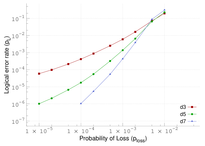
Figure 17: Logical error rate ($P_{L}$) vs. Probability of loss ($p_{loss}$). Fixed computational error ($p_{comp}=10^{-4}$) and 100% chance of loss interaction error ($p_{lint}=1$).

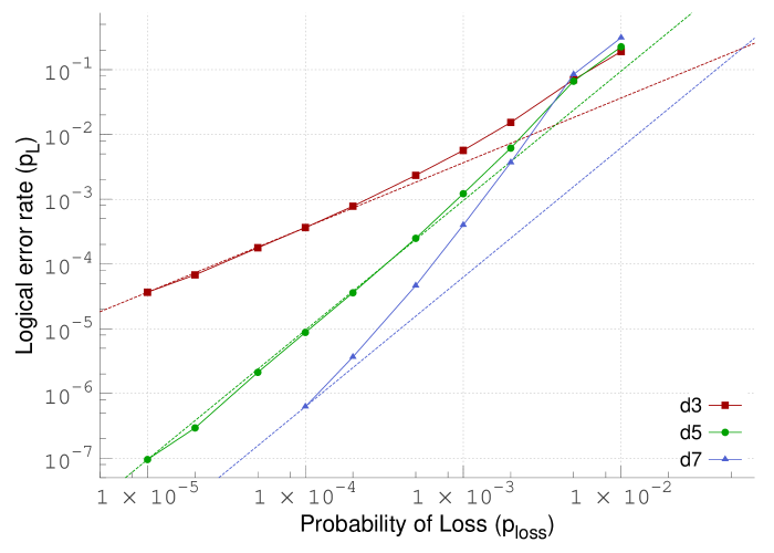
Figure 18: Logical error rate ($P_{L}$) vs. Probability of loss ($p_{loss}$). Fixed computational error ($p_{comp}=0$) and 100% chance of loss interaction error ($p_{lint}=1$). Dotted lines indicate asymptotic lines where logical errors predominantly caused by the minimum necessary ($\approx cp_{loss}^{\big{\lfloor}\frac{d+3}{4}\big{\rfloor}}$).

Overhead	$\mathbf{p_{Loss}}$	$\mathbf{d}$	$\mathbf{V}$	$\mathbf{q_{phys}}$
$1\times$	None	$31$	$3.2\times 10^{5}$	$8.6\times 10^{3}$
$1\times$	$2.0\times 10^{-3}$	$31$	$3.2\times 10^{5}$	$8.6\times 10^{3}$
$2\times$	$1.0\times 10^{-2}$	$37$	$5.6\times 10^{5}$	$1.2\times 10^{4}$
$5\times$	$2.5\times 10^{-2}$	$51$	$1.5\times 10^{6}$	$2.4\times 10^{4}$
$10\times$	$2.9\times 10^{-2}$	$67$	$3.4\times 10^{6}$	$4.1\times 10^{4}$
-	$5.0\times 10^{-2}$	-	-	-

Table 1: Table of volume and physical qubit overheads at supplied rates of loss. Computational error rate: $p_{comp}=10^{-3}$. Loss interaction error rate: $p_{lint}=0$. Target logical error rate: $P_{L}=10^{-15}.$ Higher distances extrapolated from the behavior of distances $5,7,9$.

Overhead	$\mathbf{p_{loss}}$	$\mathbf{d}$	$\mathbf{V}$	$\mathbf{q_{phys}}$
$1\times$	None	$15$	$3.4\times 10^{4}$	$1.9\times 10^{3}$
$1\times$	$5.0\times 10^{-3}$	$15$	$3.4\times 10^{4}$	$1.9\times 10^{3}$
$2\times$	$1.0\times 10^{-2}$	$19$	$7.1\times 10^{4}$	$3.1\times 10^{3}$
$8\times$	$2.0\times 10^{-2}$	$29$	$2.6\times 10^{5}$	$7.5\times 10^{3}$
$10\times$	$2.2\times 10^{-2}$	$31$	$3.2\times 10^{5}$	$8.6\times 10^{3}$
-	$5.0\times 10^{-2}$	-	-	-

Table 2: Table of volume and physical qubit overheads at supplied rates of loss. Computational error rate: $p_{comp}=10^{-4}$. Loss interaction error rate: $p_{lint}=0$. Target logical error rate: $P_{L}=10^{-15}.$ Higher distances extrapolated from the behavior of distances $5,7,9$.

Overhead	$\mathbf{p_{Loss}}$	$\mathbf{d}$	$\mathbf{V}$	$\mathbf{q_{phys}}$
$1\times$	None	$31$	$3.2\times 10^{5}$	$8.6\times 10^{3}$
$1\times$	$1.0\times 10^{-4}$	$33$	$3.9\times 10^{5}$	$9.7\times 10^{3}$
$2\times$	$2.0\times 10^{-4}$	$37$	$5.6\times 10^{5}$	$1.2\times 10^{4}$
$3\times$	$5.0\times 10^{-4}$	$45$	$1.0\times 10^{6}$	$1.8\times 10^{4}$
$10\times$	$1.0\times 10^{-3}$	$63$	$2.8\times 10^{6}$	$3.6\times 10^{4}$
-	$5.0\times 10^{-3}$	-	-	-

Table 3: Table of volume and physical qubit overheads at supplied rates of loss. Computational error rate: $p_{comp}=10^{-3}$. Loss interaction error rate: $p_{lint}=1$. Target logical error rate: $P_{L}=10^{-15}.$ Higher distances extrapolated from the behavior of distances $3,5,7$.

Overhead	$\mathbf{p_{Loss}}$	$\mathbf{d}$	$\mathbf{V}$	$\mathbf{q_{phys}}$
$1\times$	None	$15$	$3.4\times 10^{4}$	$1.9\times 10^{3}$
$1\times$	$1.0\times 10^{-5}$	$15$	$3.4\times 10^{4}$	$1.9\times 10^{3}$
$2\times$	$5.0\times 10^{-5}$	$19$	$7.1\times 10^{4}$	$3.1\times 10^{3}$
$5\times$	$2.0\times 10^{-4}$	$25$	$1.7\times 10^{5}$	$5.5\times 10^{3}$
$10\times$	$5.0\times 10^{-4}$	$33$	$3.9\times 10^{5}$	$9.7\times 10^{3}$
-	$5.0\times 10^{-3}$	-	-	-

Table 4: Table of volume and physical qubit overheads at supplied rates of loss. Computational error rate: $p_{comp}=10^{-4}$. Loss interaction error rate: $p_{lint}=1$. Target logical error rate: $P_{L}=10^{-15}.$ Higher distances extrapolated from the behavior of distances $3,5,7$.

Four tables of results were calculated, consisting of each paired combination of $p_{lint}\in\{0,1\}$ and $p_{comp}\in\{10^{-3},10^{-4}\}$. Overhead is calculated using the number of qubits necessary to create a plumbing piece achieving a given logical error rate ($P_{L}=10^{-15}$ in all instances) in comparison to the baseline with no loss ($p_{loss}=0$). The values used for the baseline are taken or extrapolated from the data presented in (Fowler et al., 2012b).

Data was collected for distances $3$, $5$, $7$ and $9$, higher distances were extrapolated from the average error suppression ratio of the two highest available distances. At low $d$, the ratios of error suppression for points near to the threshold are not expected to be constant. As a result, extrapolation at these points will underestimate the overhead. Sufficiently far from the threshold, or at large $d$, this error suppression ratio is expected to be constant (Fowler, 2012). Direct simulation and extrapolation have been compared in detail for the case of the surface code (Fowler, 2013b) with a high level of agreement when error models are not asymmetric, the case studied here.

We now provide an example of this extrapolation for clarity. To extrapolate to any distance we take the value for highest distance and divide it by the ratio of the two highest distance points the appropriate number of times. Let $a$ and $b$ be the second highest and highest distance points respectively. $d$ is the desired distance, and $d_{b}$ is the distance of the highest point.

$$p_{L}\approx\frac{b}{\left(\frac{a}{b}\right)^{\left\lfloor\frac{d-d_{b}}{2}\right\rfloor}}$$

With loss interaction errors enabled ($p_{lint}=1$), a computational error rate of $0.1\%$ ($p_{comp}=0.001$) and loss rate of $0.01\%$ ($p_{loss}=10^{-4}$) the logical error rates for distances $5$ and $7$ are $a=4.1\times 10^{-4}$ and $b=6.3\times 10^{-5}$ respectively (Fig  16). The ratio between these two points is therefore $\sim$$6.51$ and $d_{b}=7$. At distance $33$, this gives us a value for $p_{L}\approx 1.7\times 10^{-15}$ which is below our target threshold of $p_{L}=10^{-15}$.

Without loss interaction errors ($p_{lint}=0$), we find for $p_{comp}\in\{10^{-3},10^{-4}\}$ (Tables 1 & 2) that values of $p_{loss}\geq 5\%$ are clearly above threshold, with the actual threshold expected to be between $3$–$4\%$. It is observed that $\sim$$2.5\%$ loss is tolerable with $\leq 10\times$ the qubit volume required to implement the same algorithm as an identical quantum computer with no loss. For values of $p_{loss}$ above this point, the overhead rapidly increases.

The topological cluster state has the highest threshold of any code that requires only a 2D lattice of qubits with nearest-neighbor interactions, while also having a process for handling qubit loss. Despite requiring the fewest qubits to implement a logical qubit of any code under these practical hardware restrictions, the number of qubits necessary is high. Given a single logical qubit needs $\sim$$3\times 10^{4}$ qubit-rounds without loss present, we choose to consider a loss rate that more than doubles the baseline overhead to be undesirable.

An architecture with loss during initialization, two-qubit gates, and measurement should therefore highly preferably have a loss rate less than $1\%$ in order to keep the overhead under control. In order for loss to have a negligible penalty – such that there is no overhead compared to when there is no loss at all – a loss rate less than $0.5\%$ is necessary.

Due to the larger effective impact of loss when loss interaction errors can occur ($p_{lint}=1$), and the consequent reduction of the gate threshold error rate to not far above $10^{-3}$, there are more substantial differences in the overheads between $p_{comp}=10^{-3}$ (Table 3) and $p_{comp}=10^{-4}$ (Table 4). When loss interaction errors occur, values of $p_{loss}\geq 0.5\%$ are clearly above threshold, with the actual threshold expected to be between $0.3$–$0.4\%$. The maximum amount of loss tolerable with $\leq 10\times$ overhead is approximately $0.05$–$0.1\%$, with $0.001$–$0.01\%$ necessary to have no overhead.

The rate of loss tolerable while maintaining modest ($\leq 2\times$) overhead is as low as $0.005\%$ with $0.1\%$ computational error ($p_{comp}=10^{-3}$), considerably lower than when there are no loss interaction errors.

Given our focus on practical overhead, we have omitted techniques that would allow us to tolerate more loss. Techniques exist, particularly for linear optical architectures, which allow substantial improvement to the acceptable amount of loss at the cost of introducing substantial overhead (Nickerson et al., 2014; Varnava et al., 2008; Li et al., 2012).

XI Discussion

We have shown that when including loss during initialization and two-qubit gates, the amount of loss tolerable is much smaller than when only considering loss before measurement. We find that even in the best case scenario ($10^{-4}$ computational error and no errors caused when interacting with lost qubits) only $1\%$ loss can be tolerated if we allow the use of twice the qubit volume as would be required by a lossless quantum computer. The quickly increasing overhead beyond $1\%$ (threshold $3$–$4\%$) rapidly becomes highly impractical. These results, combined with the fact our results are likely to underestimate the overhead, lead us to conclude that even in the best case, no more than $1\%$ loss can be tolerated while maintaining practical overheads.

We have also demonstrated the importance of considering loss interaction errors. The creation of additional errors on neighboring qubits when they attempt to interact with a lost qubit reduces the amount of loss that is practically tolerable by at least an order of magnitude, down to $0.1\%$ for a $10$$\times$ overhead. This is due to a single loss error potentially causing a chain of two computational errors.

We have provided the first analysis of the topological cluster state for its tolerance to loss under these more detailed error models, as well as providing overhead scaling for two current experimental targets, $p_{comp}\in\{10^{-3},10^{-4}\}$. In doing so, we have shown that by ignoring initialization and two-qubit loss, previous work has overestimated the amount of loss tolerable. Our work provides concrete experimental loss targets for a range of resultant overheads, and highlights the importance of reducing or eliminating loss interaction errors.

XII Acknowledgments

This research was funded by the Australian Federal Government. This research was supported in part by the Australian Research Council Centre of Excellence for Quantum Computation and Communication Technology (project number CE110001027). AGF was funded by the US Office of the Director of National Intelligence (ODNI), Intelligence Advanced Research Projects Activity (IARPA), through the US Army Research Office grant No. W911NF-10-1-0334. All statements of fact, opinion or conclusions contained herein are those of the authors and should not be construed as representing the official views or policies of IARPA, the ODNI, or the US Government.

Appendix A Derivation of Cell State

Figure 19: A 2D representation of the 18 qubit cluster state of a single 3D topological cluster state cell (Fig. 2). Black dots are the qubits $q_{1}$ to $q_{1}8$, initialized in the $\ket{+}$ state. Black lines indicate $C_{Z}$ gates between the two connected qubits. Dotted lines are a visual guide for $C_{Z}$ gates that are not nearest neighbors in the 2D flattening.

In Table 5 we can see a set of stabilizers for the 3D topological cluster state cell (Fig. 19). This is just one possible generating set for the given cluster state. It was obtained according to the procedure outlined in Section III.

$A_{1}$	$X$	$I$	$Z$	$I$	$I$	$I$	$I$	$I$	$I$	$I$	$I$	$I$	$I$	$I$	$I$	$I$	$Z$	$I$
$A_{2}$	$I$	$X$	$Z$	$I$	$I$	$I$	$I$	$I$	$I$	$Z$	$I$	$I$	$I$	$I$	$I$	$I$	$I$	$I$
$A_{3}$	$Z$	$Z$	$X$	$Z$	$Z$	$I$	$I$	$I$	$I$	$I$	$I$	$I$	$I$	$I$	$I$	$I$	$I$	$I$
$A_{4}$	$I$	$I$	$Z$	$X$	$I$	$I$	$I$	$I$	$I$	$I$	$I$	$I$	$I$	$Z$	$I$	$I$	$I$	$I$
$A_{5}$	$I$	$I$	$Z$	$I$	$X$	$I$	$Z$	$I$	$I$	$I$	$I$	$I$	$I$	$I$	$I$	$I$	$I$	$I$
$A_{6}$	$I$	$I$	$I$	$I$	$I$	$X$	$Z$	$I$	$I$	$Z$	$I$	$I$	$I$	$I$	$I$	$I$	$I$	$I$
$A_{7}$	$I$	$I$	$I$	$I$	$Z$	$Z$	$X$	$Z$	$Z$	$I$	$I$	$I$	$I$	$I$	$I$	$I$	$I$	$I$
$A_{8}$	$I$	$I$	$I$	$I$	$I$	$I$	$Z$	$X$	$I$	$I$	$I$	$I$	$I$	$Z$	$I$	$I$	$I$	$I$
$A_{9}$	$I$	$I$	$I$	$I$	$I$	$I$	$Z$	$I$	$X$	$I$	$I$	$Z$	$I$	$I$	$I$	$I$	$I$	$I$
$A_{10}$	$I$	$Z$	$I$	$I$	$I$	$Z$	$I$	$I$	$I$	$X$	$Z$	$I$	$I$	$I$	$I$	$Z$	$I$	$I$
$A_{11}$	$I$	$I$	$I$	$I$	$I$	$I$	$I$	$I$	$I$	$Z$	$X$	$Z$	$I$	$I$	$I$	$I$	$I$	$I$
$A_{12}$	$I$	$I$	$I$	$I$	$I$	$I$	$I$	$I$	$Z$	$I$	$Z$	$X$	$Z$	$I$	$Z$	$I$	$I$	$I$
$A_{13}$	$I$	$I$	$I$	$I$	$I$	$I$	$I$	$I$	$I$	$I$	$I$	$Z$	$X$	$Z$	$I$	$I$	$I$	$I$
$A_{14}$	$I$	$I$	$I$	$Z$	$I$	$I$	$I$	$Z$	$I$	$I$	$I$	$I$	$Z$	$X$	$I$	$I$	$I$	$Z$
$A_{15}$	$I$	$I$	$I$	$I$	$I$	$I$	$I$	$I$	$I$	$I$	$I$	$Z$	$I$	$I$	$X$	$I$	$Z$	$I$
$A_{16}$	$I$	$I$	$I$	$I$	$I$	$I$	$I$	$I$	$I$	$Z$	$I$	$I$	$I$	$I$	$I$	$X$	$Z$	$I$
$A_{17}$	$Z$	$I$	$I$	$I$	$I$	$I$	$I$	$I$	$I$	$I$	$I$	$I$	$I$	$I$	$Z$	$Z$	$X$	$Z$
$A_{18}$	$I$	$I$	$I$	$I$	$I$	$I$	$I$	$I$	$I$	$I$	$I$	$I$	$I$	$Z$	$I$	$I$	$Z$	$X$

Table 5: A set of stabilizers for a single 3D topological cluster state cube, containing one for each of the 18 qubits. After the application of the $C_{Z}$ gates, the cell will be simultaneously in the $+1$ eigenstate of each of these stabilizers.

If we select the stabilizers we have created based on each of the face qubits, $A_{3}$, $A_{7}$, $A_{10}$, $A_{12}$, $A_{14}$ and $A_{17}$ (Table 6). It can be seen, that each column of the stabilizer generating set contains either a single $\hat{X}$ operator, or two $\hat{Z}$ operators and $\hat{I}$ on the remainder.

$A_{3}$	$Z$	$Z$	$X$	$Z$	$Z$	$I$	$I$	$I$	$I$	$I$	$I$	$I$	$I$	$I$	$I$	$I$	$I$	$I$
$A_{7}$	$I$	$I$	$I$	$I$	$Z$	$Z$	$X$	$Z$	$Z$	$I$	$I$	$I$	$I$	$I$	$I$	$I$	$I$	$I$
$A_{10}$	$I$	$Z$	$I$	$I$	$I$	$Z$	$I$	$I$	$I$	$X$	$Z$	$I$	$I$	$I$	$I$	$Z$	$I$	$I$
$A_{12}$	$I$	$I$	$I$	$I$	$I$	$I$	$I$	$I$	$Z$	$I$	$Z$	$X$	$Z$	$I$	$Z$	$I$	$I$	$I$
$A_{14}$	$I$	$I$	$I$	$Z$	$I$	$I$	$I$	$Z$	$I$	$I$	$I$	$I$	$Z$	$X$	$I$	$I$	$I$	$Z$
$A_{17}$	$Z$	$I$	$I$	$I$	$I$	$I$	$I$	$I$	$I$	$I$	$I$	$I$	$I$	$I$	$Z$	$Z$	$X$	$Z$

Table 6: A subset of the stabilizers for a single 3D topological cluster state cube. Specifically, the subset that were stabilizing each of the center face qubits of the 3D topological cluster state cell.

If we then take the matrix product of these stabilizers we can form a new stabilizer, $A$ (Table 7). Given that $(A_{1}\otimes B_{2})\cdot(C_{1}\otimes D_{2})=(A_{1}\cdot C{{}_{1}})\otimes(B_{2}\cdot D_{2})$, the $\hat{Z}$ operators will all cancel (as the inverse of $\hat{Z}$ is $\hat{Z}$) and we will be left with a new stabilizer with $\hat{X}$ operators on the face qubits ($q_{3}$, $q_{7}$, $q_{10}$, $q_{12}$, $q_{14}$ and $q_{17}$) and $I$ on the others.

$A$	$I$	$I$	$X$	$I$	$I$	$I$	$X$	$I$	$I$	$X$	$I$	$X$	$I$	$X$	$I$	$I$	$X$	$I$

Table 7: A new stabilizer $A$ that is the matrix product of $A_{3}$, $A_{7}$, $A_{10}$, $A_{12}$, $A_{14}$ and $A_{17}$. This can replace any of the 6 stabilizers to form a new valid set of stabilizers.

If we measure the new stabilizer $A$ (by measuring the face qubits in the $\hat{X}$ basis), in the absence of errors, each qubit will be in either the $+1$ or $-1$ eigenstate of $\hat{X}$. On the whole however, the result will be the $+1$ eigenstate of the stabilizer $A$. Therefore, if you take the product of each of the measurement results, the result (in the absence of error) will be $+1$. It is important to note that the stabilizer $A$ does not force each qubit to be in the $+1$ eigenstate of $\hat{X}$, only that the measurement product of all six face qubits be $+1$.

The reason we chose the stabilizers $A_{3}$, $A_{7}$, $A_{10}$, $A_{12}$, $A_{14}$ and $A_{17}$ is because we can only measure in a single basis simultaneously. Therefore, we want a stabilizer that consists of only $\hat{X}$ or only $\hat{Z}$ operators. The stabilizers chosen are the easiest way to obtain this given the method of generating the initial set of stabilizers for the 3D topological cluster cell state.

References

- Barrett and Stace (2010) S. D. Barrett and T. M. Stace, Phys. Rev. Lett. 105, 200502 (2010), arXiv:1005.2456v2.
- Fowler et al. (2012a) A. G. Fowler, A. C. Whiteside, and L. C. L. Hollenberg, Phys. Rev. Lett. 108, 180501 (2012a), arXiv:1110.5133v2.
- Bravyi and Kitaev (1998) S. B. Bravyi and A. Y. Kitaev, arXiv:quant-ph/9811052 (1998).
- Fortescue et al. (2014) B. Fortescue, S. Nawaf, and M. Byrd, arXiv:1405.1766v1 (2014).
- Vala et al. (2005) J. Vala, K. B. Whaley, and D. S. Weiss, Physical Review A 72, 052318 (2005), arXiv:quant-ph/0510021v1.
- Blakestad et al. (2011) R. B. Blakestad, C. Ospelkaus, A. P. VanDevender, J. H. Wesenberg, M. J. Biercuk, D. Leibfried, and D. J. Wineland, Physical Review A 84, 032314 (2011), arXiv:1106.5005v1.
- Wright et al. (2013) K. Wright, J. M. Amini, D. L. Faircloth, C. Volin, S. C. Doret, H. Hayden, C.-S. Pai, D. W. Landgren, D. Denison, T. Killian, R. E. Slusher, and A. W. Harter, New J. Phys. 15, 033004 (2013), arXiv:1210.3655.
- Raussendorf et al. (2003) R. Raussendorf, D. E. Browne, and H. J. Briegel, Physical Review A 68, 022312 (2003), arXiv:quant-ph/0301052v2.
- Fowler et al. (2012b) A. G. Fowler, A. C. Whiteside, A. L. McInnes, and A. Rabbani, Phys. Rev. X 2, 041003 (2012b), arXiv:1202.6111, http://topqec.com.au/autotune.html.
- Knill et al. (2000) E. Knill, R. Laflamme, and G. Milburn, arXiv:quant-ph/0006088v1 (2000), arXiv:quant-ph/0006088v1.
- Mandel et al. (2003) O. Mandel, M. Greiner, A. Widera, T. Rom, T. W. Hänsch, and I. Bloch, Nature 425, 937 (2003), arXiv:quant-ph/0308080v1.
- Olmschenk et al. (2010) S. Olmschenk, R. Chicireanu, K. D. Nelson, and J. V. Porto, New J. Phys. 12, 113007 (2010), arXiv:1008.2790v2.
- Herrera-Marti et al. (2010) D. A. Herrera-Marti, A. G. Fowler, D. Jennings, and T. Rudolph, Phys. Rev. A 82, 032332 (2010), arXiv:1005.2915v1.
- Gottesman (1997) D. Gottesman, arXiv:quant-ph/9705052v1 (1997).
- Aaronson and Gottesman (2004) S. Aaronson and D. Gottesman, Physical Review A 70, 052328 (2004), arXiv:quant-ph/0406196v5.
- Anders and Briegel (2006) S. Anders and H. J. Briegel, Physical Review A 73, 022334 (2006), arXiv:quant-ph/0504117v2.
- Fowler and Goyal (2009) A. G. Fowler and K. Goyal, Quant. Info. Comput. 9, 721 (2009), arXiv:0805.3202v2.
- Edmonds (1965) J. Edmonds, Journal of Research of the National Bureau of Standards Section B Mathematics and Mathematical Physics 69B, 125 (1965), 10.6028/jres.069b.013.
- Fowler (2013a) A. G. Fowler, arXiv:1307.1740v2 (2013a).
- Duclos-Cianci and Poulin (2010) G. Duclos-Cianci and D. Poulin, Phys. Rev. Lett. 104, 050504 (2010).
- Duclos-Cianci and Poulin (2014) G. Duclos-Cianci and D. Poulin, Quant. Inf. Comp. 14, 0721 (2014), arXiv:1304.6100v1.
- Wootton and Loss (2012) J. R. Wootton and D. Loss, Phys. Rev. Lett. 109, 160503 (2012), arXiv:1202.4316.
- Hutter et al. (2014) A. Hutter, J. R. Wootton, and D. Loss, Physical Review A 89, 022326 (2014), arXiv:1302.2669v2.
- Bombin et al. (2012) H. Bombin, R. S. Andrist, M. Ohzeki, H. G. Katzgraber, and M. A. Martin-Delgado, Phys. Rev. X 2, 021004 (2012), arXiv:1202.1852v2.
- Bravyi et al. (2014) S. Bravyi, M. Suchara, and A. Vargo, arXiv:1405.4883v1 (2014).
- Raussendorf and Harrington (2007) R. Raussendorf and J. Harrington, Phys. Rev. Lett. 98, 190504 (2007), arXiv:quant-ph/0610082v2.
- Raussendorf et al. (2007) R. Raussendorf, J. Harrington, and K. Goyal, New J. Phys. 9, 199 (2007), arXiv:quant-ph/0703143v1.
- Kolmogorov (2009) V. Kolmogorov, Mathematical Programming Computation 1, 43 (2009), 10.1007/s12532-009-0002-8.
- Fowler et al. (2012c) A. G. Fowler, A. C. Whiteside, and L. C. L. Hollenberg, Physical Review A 86, 042313 (2012c), arXiv:1202.5602v2.
- Fowler et al. (2014) A. G. Fowler, D. Sank, J. Kelly, R. Barends, and J. M. Martinis, arXiv:1405.1454v1 (2014).
- Fowler (2012) A. G. Fowler, Phys. Rev. Lett. 109, 180502 (2012), arXiv:1206.0800v2.
- Fowler (2013b) A. G. Fowler, arXiv:1307.0689v1 (2013b).
- Nickerson et al. (2014) N. H. Nickerson, J. F. Fitzsimons, and S. C. Benjamin, arXiv:1406.0880v1 (2014).
- Varnava et al. (2008) M. Varnava, D. E. Browne, and T. Rudolph, Phys. Rev. Lett. 100, 060502 (2008), arXiv:quant-ph/0702044v2.
- Li et al. (2012) Y. Li, S. D. Barrett, T. M. Stace, and S. C. Benjamin, arXiv:1209.4031v1 (2012).