Backward Raman amplification in the Langmuir wavebreaking regime

Abstract

In plasma-based backward Raman amplifiers, the output pulse intensity increases with the input pump pulse intensity, as long as the Langmuir wave mediating energy transfer from the pump to the seed pulse remains intact. However, at high pump intensity, the Langmuir wave breaks, at which point the amplification efficiency may no longer increase with the pump intensity. Numerical simulations presented here, employing a 1D Vlasov-Maxwell code, show that, although the amplification efficiency remains high when the pump only mildly exceeds the wavebreaking threshold, the efficiency drops precipitously at larger pump intensities.

I Introduction

The largest laser powers are currently produced through chirped pulse amplification (CPA) technique Mourou85 ; Mourou98 (see also a recent review Yakovlev_14 ). The power limit in CPA technique comes from the final material gratings needed to re-compress the amplified pulse (which was stretched before the amplification). Material gratings apparently cannot tolerate laser pulses so intense that the electron quiver energy reaches the material ionization energy. For laser wavelengths on the order of a micron, this limits the maximum laser intensity on gratings to a few TW$/$cm².

However, the maximum output in intensities reachable through backward Raman amplification (BRA) of laser pulses in plasma can, in principle, be nearly 10⁶ times larger Malkin_99_PRL ; Malkin_00_POP ; Fisch_03_POP ; Malkin_05_POP . The BRA employs the resonant 3-wave decay of the pump laser pulse into the counter-propagating seed laser pulse and the Langmuir wave. The seed pulse captures substantial fraction of the pump energy and contracts reaching nearly relativistic intensities. Several other plasma-based mechanisms have also been proposed to compress laser pulses in a counter-propagating geometry. These mechanisms include Compton backscattering Shvets_98_PRL or, more recently, strongly-coupled Brilliouin backscattering Weber_06 ; PRL-2010-Lancia ; PRL-2013-Weber , or possibly a combination of Raman and Brilliouin backscattering Riconda_13 . However, at present, the BRA has enjoyed the most theoretical and experimental development, and appears to be the most promising for high intensity applications.

Inasmuch as the energy transfer in BRA is mediated by the Langmuir wave, the BRA efficiency can be significantly reduced by Langmuir wavebreaking Malkin_99_PRL ; Malkin_00_POP ; Malkin_14-EPJST , which occurs when the longitudinal quiver electron velocity exceeds the phase velocity of the Langmuir wave  Dawson_59 ; Kruer1988 . Apart from the Langmuir wave breaking, the BRA efficiency might be impeded by the amplified pulse filamentation and detuning due to the relativistic electron nonlinearity Malkin_99_PRL ; Fraiman_02_POP ; Malkin_07_PRL ; 2012-dispersion ; Malkin_14-EPJST ; PoP-2014-Lehmann , parasitic Raman scattering of the pump and amplified pulses by plasma noise Malkin_99_PRL ; Malkin_00_PRL ; Malkin_00_POP ; Tsidulko_00_PRL ; Solodov_04_PRE ; Malkin_14-EPJST , generation of superluminous precursors of the amplified pulse Tsidulko_02_PRL , pulse scattering by plasma density inhomogeneities Solodov_dens , pulse depletion and plasma heating through inverse bremsstrahlung Malkin_07_PRE ; Malkin_09_PRE ; Malkin_10_POP ; 2011-Balakin , and resonant Langmuir wave Landau damping PRL-2005-Hur ; Malkin_07_PRE ; PoP-2009-Yampolsky ; Malkin_10_POP ; PoP-2011-Yampolsky ; PoP-2012-Strozzi ; IEEE-2014-Wu ; NatCom-2014-Depierreux . Taking into account these impediments to high efficiency, the regimes of the met robust efficiency can be identified Clark_03_POP ; Yampolsky_04_PRE ; Toroker_POP_12 ; Toroker_12_PRL .

In the regimes in which the wavebreaking is not too strong, the BRA effect was demonstrated experimentally Ping_00_PRE ; Ping_02_PRE ; Ping_04_PRL ; Balakin_04_JETPL ; Cheng_05_PRL ; Ren_08_POP ; Jaro_12_NJP ; Jaro_12_SPI . The experiments also indicated that the maximum BRA efficiency is achieved at pump intensities not exceeding by much the wavebreaking threshold PoP-2011-Yampolsky , in accordance with the theoretical expectations Malkin_99_PRL .

Note that, apart from the issue of efficiency, there might be advantages to operating in the parameter regime prone to strong wavebreaking. For example, having larger laser-to-plasma frequency ratio (at which the Langmuir phase velocity is smaller) may reduce the parasitic Raman forward scattering of the amplified pulse Malkin_99_PRL ; Malkin_00_PRL ; Malkin_00_POP , while larger pump intensities might enable the amplified pulse to grow faster. The combination of these factors can incur strong wavebreaking.

Thus, it would be important if there were any possibility to increase the efficiency in strong wavebreaking regimes. This would be primarily important around the optical range. For UV and X-ray regimes Malkin_07_PRE ; Malkin_09_PRE , the wavebreaking intensities are already very high and not readily attainable at any Langmuir wave phase velocity exceeding a realistic thermal electron velocity, i.e. in the entire realistic range of the Langmuir wave existence. Recently in PIC simulations in the optical frequency range, high BRA efficiency was in fact reported in a very strong wavebreaking regime Trines_10 . One of our purposes here was to confirm, in a different code, this optimistic prediction. However, while the efficiencies obtained here are in agreement with most of the efficiencies reported in the recent PIC simulations, they do not confirm the very high efficiency in the very strong wavebreaking regime.

Our paper explores the wavebreaking regimes numerically using the Vlasov-Maxwell (VM) code described below. First, we verify this code below wavebreaking. Then we apply this code to the pump pulse intensities exceeding the wavebreaking threshold. For mild wavebreaking regimes, where the pump intensities that exceed the wavebreaking threshold by no more than a factor of just several, the VM code results are in agreement with both analytic calculations and previous PIC simulations. In this regime, highly efficient backward Raman amplification is still possible. For the strong wavebreaking regimes, we find that the BRA efficiency there basically agrees with both the analytical estimates of Ref. Malkin_99_PRL, and numerical results of Fig. 3a of Ref. Trines_10, , but is at variance with much higher BRA efficiency of Fig. 2a of Ref. Trines_10, . In addition, we show that the BRA efficiency in the mild wavebreaking regime can be noticeably increased by increasing the input seed pulse intensity, while the BRA efficiency in the strong wavebreaking regime is basically not affected by increasing the input seed pulse intensity.

II Model description

To analyze the BRA wavebreaking regimes, we employ a one-dimensional (1D) relativistic Vlasov-Maxwell (VM) code. The non-relativistic version of this code can be found in  Bert_90 ; Cheng_76 ; Reveille_92 ; Ghizzo_95 . The VM code is applicable to the BRA both below and above the wavebreaking threshold. In particular, below the threshold, this code covers the parameter range where the fluid description of the BRA is applicable, while, above the threshold, this code can properly handle kinetic effects important there. We solve full Maxwell equations, not using an envelope approximation for waves (even though it would much reduce the computational overhead and might be particularly useful for simulating multidimensional effects Farmer_13 ), because the validity of the envelope approximations in the strong wavebreaking regime might still need to be verified independently.

The pump and seed pulses, counter-propagating the direction $\hat{z}$, are comprised of transverse electric and magnetic fields linearly polarized in $\hat{x}$ and $\hat{y}$ directions, respectively, $\vec{\bar{E}}=\bar{E}_{x}\hat{x}$ and $\vec{\bar{B}}=\bar{B}_{y}\hat{y}$. The seed pulse frequency $\omega_{b}$ is down-shifted from the pump frequency $\omega_{a}$ by the electron plasma frequency $\omega_{e}=\sqrt{4\pi n_{e0}e^{2}/m_{e}}$, so that the Langmuir wave is resonantly excited, having the longitudinal electric field $\vec{\bar{E}}=\bar{E}_{z}\hat{z}$. The fields are measured in units $m_{e}c\omega_{e}/e$, $m_{e}$ is the electron mass, $-e$ is the electron charge, $n_{e0}$ is the initial electron plasma concentration and $c$ is the speed of light in vacuum. The time $\bar{t}$ is measured further in units $1/\omega_{e}$ and the distance $\bar{z}$ is measured in units $c/\omega_{e}$. We also define the dimensionless frequencies $\bar{\omega}_{a}=\omega_{a}/\omega_{e}$ and $\bar{\omega}_{b}=\omega_{b}/\omega_{e}$ , and the respective dimensionless wavenumbers $\bar{k}_{a}=\sqrt{\bar{\omega}_{a}^{2}-1}$ and $\bar{k}_{b}=\sqrt{\bar{\omega}_{b}^{2}-1}$. The resonant Langmuir wave then has the dimensionless wavenumber $\bar{k}_{f}=\bar{k}_{a}+\bar{k}_{b}$.

For the fast laser-plasma interaction of interest here, the slow ion motion can be neglected. The longitudinal electron distribution function $\bar{f}$ is described by the one-dimensional Vlasov equation,

$$\frac{\partial{\bar{f}}}{\partial{\bar{t}}}+\frac{\bar{p}_{z}}{\bar{\gamma}}\frac{\partial\bar{f}}{\partial\bar{z}}-(\bar{E}_{z}+\frac{\bar{P}_{x}}{\bar{\gamma}}\bar{B}_{y})\frac{\partial\bar{f}}{\partial\bar{p}_{z}}=0,$$ (1)

where $\bar{\gamma}=\sqrt{1+\bar{P}_{x}^{2}+\bar{p}_{z}^{2}}$ is the Lorentz factor, $\bar{P}_{x}$ and $\bar{p}_{z}$ are the electron momentum components in the $\hat{x}$ and $\hat{z}$ directions, respectively, measured in units $m_{e}c$. The distribution function $\bar{f}$ is measured in units $n_{e0}/m_{e}c$.

The electrostatic field $\bar{E}_{z}=-\partial\bar{\phi}/\partial\bar{z}$ is found by solving Poisson’s equation

$$\frac{\partial^{2}\bar{\phi}}{\partial\bar{z}^{2}}=-[1-\bar{n}_{e}(\bar{z},\bar{t})],$$ (2)

where $\bar{n}_{e}(\bar{z},\bar{t})=\int\bar{f}(\bar{z},\bar{p}_{z},\bar{t})d\bar{p}_{z}$ is the electron concentration normalized to $n_{e0}$.

In this model, the electron motion in $\hat{x}$ direction is described by the fluid equation

$$\frac{\partial\bar{P}_{x}}{\partial\bar{t}}=-\bar{E}_{x}.$$ (3)

The electromagnetic waves are described by equations

$$(\frac{\partial}{\partial\bar{t}}\pm\frac{\partial}{\partial\bar{z}})\bar{E}^{\pm}=\int d\bar{p}_{z}\frac{\bar{P}_{x}}{\bar{\gamma}}\bar{f},$$ (4)

where $\bar{E}^{\pm}=\bar{E}_{x}\pm\bar{B}_{y}$. The model Eqs. (1-4) conserves energy,

$$\frac{\partial}{\partial\bar{t}}(W_{em}+W_{es}+W_{k})=0,$$ (5)

where $W_{em}=\int d\bar{z}(\bar{E}_{x}^{2}+\bar{B}_{y}^{2})/2$ is the electromagnetic energy, $W_{es}=\int d\bar{z}\bar{E}_{z}^{2}/2$ is the electrostatic energy, and $W_{k}=\int d\bar{z}\int d\bar{p}_{z}(\bar{\gamma}-1)\bar{f}$ is the kinetic energy of the electrons. The model presented here is similar to that of Ref. Lehmann_13 .

In order to avoid electromagnetic wave reflections from boundaries, perfectly matching damping layers (PML) Bere_94 ; Gedney_96 are inserted at both plasma edges. In order to avoid the Langmuir wave reflection, a Krook Krook_56 operator is added to the Vlasov equation that causes the electron distribution function $\bar{f}$ to relax to the initial distribution $\bar{f}_{0}$ in narrow boundary layers. To exclude extra spatial length from the numerical simulations, we solve the VM equations in the window around the seed pulse, using variables

$$\xi=\bar{z}+\bar{t}\,,\;\;\;\;\tau=\bar{t}\,.$$

Most of numerical examples will be presented below for the laser-to-plasma frequency ratio $\bar{\omega}_{b}=20$ and the initial electron temperature $T_{e0}=10\,eV$. This temperature is much smaller than the energy of electron moving with the resonant Langmuir wave phase velocity, $v_{\rm ph}=\omega_{e}/k_{f}\approx c/40$, which energy is $m_{e}v^{2}_{\rm ph}/2\approx 160\,eV$. In such a plasma, the wavebreaking occurs when the amplitude of the longitudinal electron quiver velocity, $eE_{L}/(m_{e}\omega_{e})$ exceeds $v_{\rm ph}$. The amplitude of the Langmuir wave electric field $E_{L}$ at the wavebreaking threshold is then

$$E_{L}=\frac{m_{e}c\,\omega_{e}^{2}}{2e\,\omega_{a}}\;.$$ (6)

The pump intensity at the Langmuir wavebreaking threshold can be evaluated as in Malkin_99_PRL ; Malkin_14-EPJST . Namely, the pump depleted energy is $\bar{\omega}_{a}\;(\approx 20)$ times larger than the energy transfered to the Langmuir wave (since decay of one pump photon produces one Langmuir plasmon of $\bar{\omega}_{a}$ smaller energy). Therefore, to produce the Langmuir wavebreaking in initially quiet plasma, the input pump intensity $I_{0}$ should necessarily exceed the critical wavebreaking value $I_{\rm br}$,

$$I_{0}>I_{\rm br}=\frac{c\,\bar{\omega}_{a}}{16\pi}\left|E_{L}\right|^{2}=\frac{m_{e}n_{e}c^{3}}{16\,\bar{\omega}_{a}}\,.$$ (7)

For the pump of wavelength $\lambda_{a}=0.8$ $\mu$m and $\bar{\omega}_{a}=20$, the wavebreaking threshold is $I_{br}=33.6$ TW$/$cm². The respective amplitude of the electron quiver velocity in the pump field is $\bar{v}_{\rm br}=(2\bar{\omega}_{a})^{-3/2}=0.004$.

We will use the Gaussian input seed pulse of the form

$$\bar{E}_{\rm seed}(\xi,\tau)=\bar{v}_{eb,0}\bar{\omega}_{b}\exp[-(\xi-\xi_{0})^{2}/2\Delta_{b}^{2}].$$ (8)

In most of the examples below the input seed pulse intensity is 10 PW$/$cm², corresponding to $\bar{v}_{eb,0}=0.07$, $\Delta_{b}=2\pi$ (i.e., the seed duration is one plasma period), and $\xi_{0}=130$.

The seed pulse is also characterized by the integrated seed amplitudeMalkin_99_PRL ; Toroker_12_PRL

$$U_{in}=\sqrt{\pi\bar{\omega}_{a}}\bar{v}_{eb,0}\Delta_{b},$$ (9)

which, for the above parameters, is $U_{in}=3.5$.

We will calculate the relative pump depletion, $\eta$, far enough behind the seed, at $\xi=200$,

$$\eta=1-\frac{\left|\bar{v}_{ea}(\xi=200,\tau=100)\right|^{2}}{\left|\bar{v}_{ea,0}\right|^{2}}$$ (10)

(here $\bar{v}_{ea}=\bar{E}_{a}/\bar{\omega}_{a}$ is the amplitude of the electron quiver velocity in the pump field, $\bar{E}_{a}$ is the electric field amplitude of the pump, and $\bar{v}_{ea,0}$ is the input value of $\bar{v}_{ea}$).

III BRA below the wavebreaking threshold

Consider first the well-studied case of BRA mediated by intact Langmuir wave. Let the input pump intensity be 4 times below the wavebreaking threshold (so that $\bar{v}_{ea,0}=0.5v_{\rm br})$. The pump is rectangular, injected in the positive $\xi$-direction and the front is initially located at $\xi=100$. In variables ($\xi,\tau$), the seed is not moving, while the pump propagates with the speed $2$. Figure. 1 shows the transverse and longitudinal electric fields $\bar{E}_{x}$ and $\bar{E}_{z}$ at $\tau=140$. As seen, most of pump is depleted behind the seed pulse ($\xi>150$).

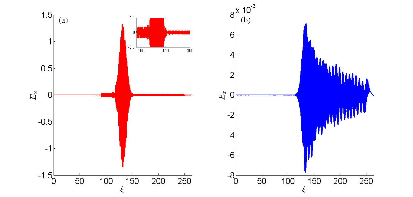
Figure 1: (Color online) The dimensionless transverse electric field, $\bar{E}_{x}$ (Fig. 1a), and longitudinal electric field, $\bar{E}_{z}$ (Fig. 1b), at the time $\tau=140$ for the input pump intensity 4 times below the wavebreaking threshold and the input seed pulse intensity 10 PW$/$cm².

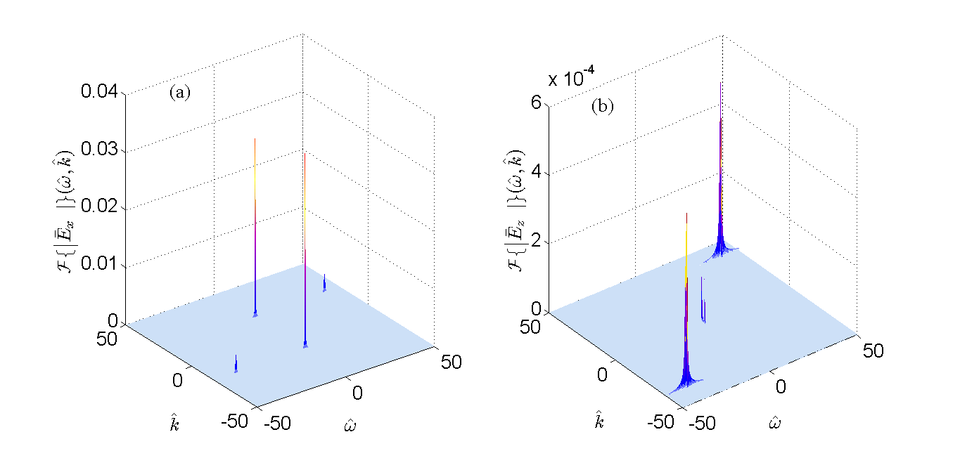
Figure 2: (Color online) The time-space Fourier-transformed transverse, $\bar{E}_{x}$ (Fig. 2a), and longitudinal, $\bar{E}_{z}$ (Fig. 2b), electric fields.

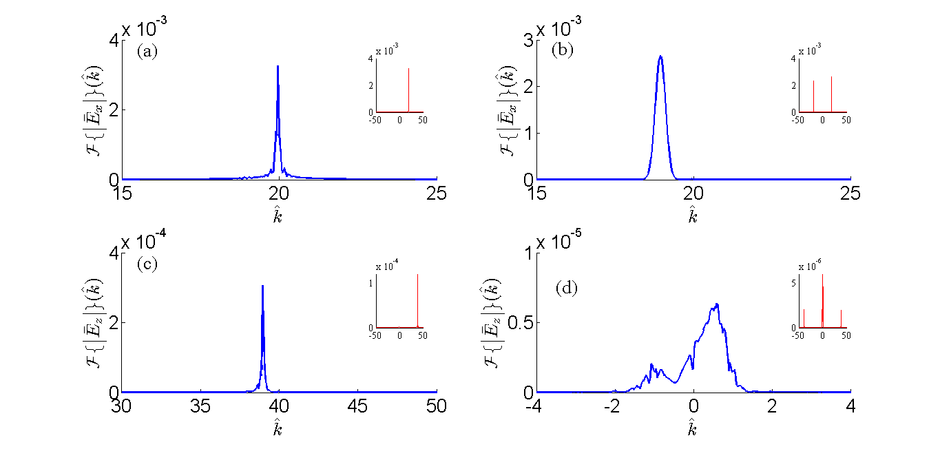
Figure 3: (Color online) The envelope of space Fourier-transformed transverse electric field, $\bar{E}_{x}$, at the frequency $\hat{\omega}=40$ (Fig. 3a) and $\hat{\omega}=0$ (Fig. 3b). The envelope of space Fourier-transformed longitudinal electric field, $\bar{E}_{z}$, at the frequency $\hat{\omega}=40$ (Fig. 3c) and $\hat{\omega}=0$ (Fig. 3d).

To separate electromagnetic fields of different waves,we use Fourier transformation. In the variables ($\xi,\tau$), the wavenumbers are the same as in ($\bar{z},\bar{t}$), while frequencies of the pump, seed and Langmuir wave are, respectively, $\hat{\omega}_{a}=\bar{\omega}_{a}+\bar{k}_{a}$, $\hat{\omega}_{b}=\bar{\omega}_{b}-\bar{k}_{b}$ and $\hat{\omega}_{f}=\bar{\omega}_{e}+\bar{k}_{f}$. For $\bar{\omega}_{a}=20$, the frequencies and wave numbers are $\hat{\omega}_{a}\approx 40$, $\hat{k}_{a}\approx 20$, $\hat{\omega}_{b}\approx 0$, $\hat{k}_{b}\approx-19$, $\hat{\omega}_{f}\approx 40$, and $\hat{k}_{f}\approx 39$. Figure 2 shows the ($\hat{k}$, $\hat{\omega}$) Fourier-transformed fields $\bar{E}_{x}$ and $\bar{E}_{z}$. Two major spikes in the Fig. 2a for the Fourier-transformed transverse field $\bar{E}_{x}$, located at $(\hat{k},\hat{\omega})=(20,40)$ and $(-20,-40)$, correspond to the pump pulse, while two lesser spikes at $(\hat{k},\hat{\omega})=(19,0)$ and $(-19,0)$ correspond to the seed pulse. Fig. 2b for the Fourier-transformed longitudinal field $\bar{E}_{z}$ contains 2 major spikes, located at $(\hat{k},\hat{\omega})=(39,40)$ and $(\hat{k},\hat{\omega})=(-39,-40)$, corresponding to the resonant Langmuir wave that mediates BRA. There are also 2 lesser spikes, located at $(\hat{k},\hat{\omega})=(1,0)$ and $(\hat{k},\hat{\omega})=(-1,0)$, corresponding to the Langmuir wave that mediates forward Raman scattering of the seed pulse. Fig. 3 shows envelopes of the spatial Fourier-transformed fields $\bar{E}_{x}$ (Figs. 3a and b) and $\bar{E}_{z}$ (Figs. 3c and d) at frequencies $\hat{\omega}=40$ (Figs. 3a and c) and $0$ (Figs. 3b and d). These correspond to the pump (Figs. 3a), seed (Figs. 3b) and Langmuir waves mediating BRA (Figs. 3c) and forward Raman scattering of seed pulse (Figs. 3d).

The pump, seed and Langmuir wave envelopes can be restored from the $(\hat{k},\hat{\omega})$ Fourier images using the Hilbert transform technique HilbTrans . These envelopes are shown in Fig. 4a. The pump behind the seed pulse is depleted by $90\%$. The incomplete pump depletion can be caused by the parasitic forward Raman scattering of the seed pulse and other deleterious processes. Fig. 4b shows the longitudinal electron momentum distribution function, $\bar{f}$, at $\tau=140$. For $\xi<130$, no interaction occurs between the pump and the seed, and the distribution function stays close to the initial Maxwellian. For $\xi>130$, the Langmuir wave is excited, and the distribution function is close to an oscillating Maxwellian, as it should be.

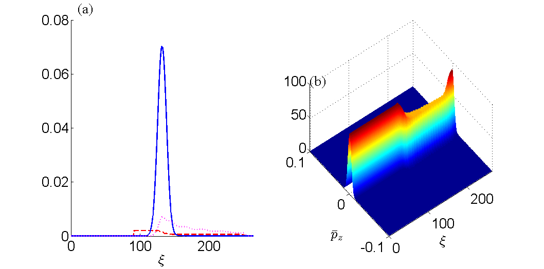
Figure 4: (Color online) Envelopes of electron quiver velocities $\bar{v}_{ea}$, $\bar{v}_{eb}$ and $\bar{v}_{ef}$ in the pump (dashed line), seed (solid line) and Langmuir wave (dotted line) fields at $\tau=140$ (Fig. 4a). Fig. 4b shows the longitudinal electron momentum distribution function.

IV BRA in wavebreaking regimes

We’ll now compare a mild wavebreaking regime, say with $\bar{v}_{ea}/\bar{v}_{br}=1.5$, i.e., the input pump intensity $2.25$ times above the wavebreaking threshold, to a strong wavebreaking regime with $\bar{v}_{ea}/\bar{v}_{br}=5.5$, i.e., the input pump intensity 30 times above the wavebreaking threshold.

Figure 5 shows the transverse and longitudinal field amplitudes in these two regimes at $\tau=90$. Despite the wavebreaking, the longitudinal field still appears to be larger at the larger pump intensity. Nevertheless, the pump depletion behind the seed pulse drops from 30$\%$ in the mild wavebreaking regime down to 9$\%$ in the strong wavebreaking regime.

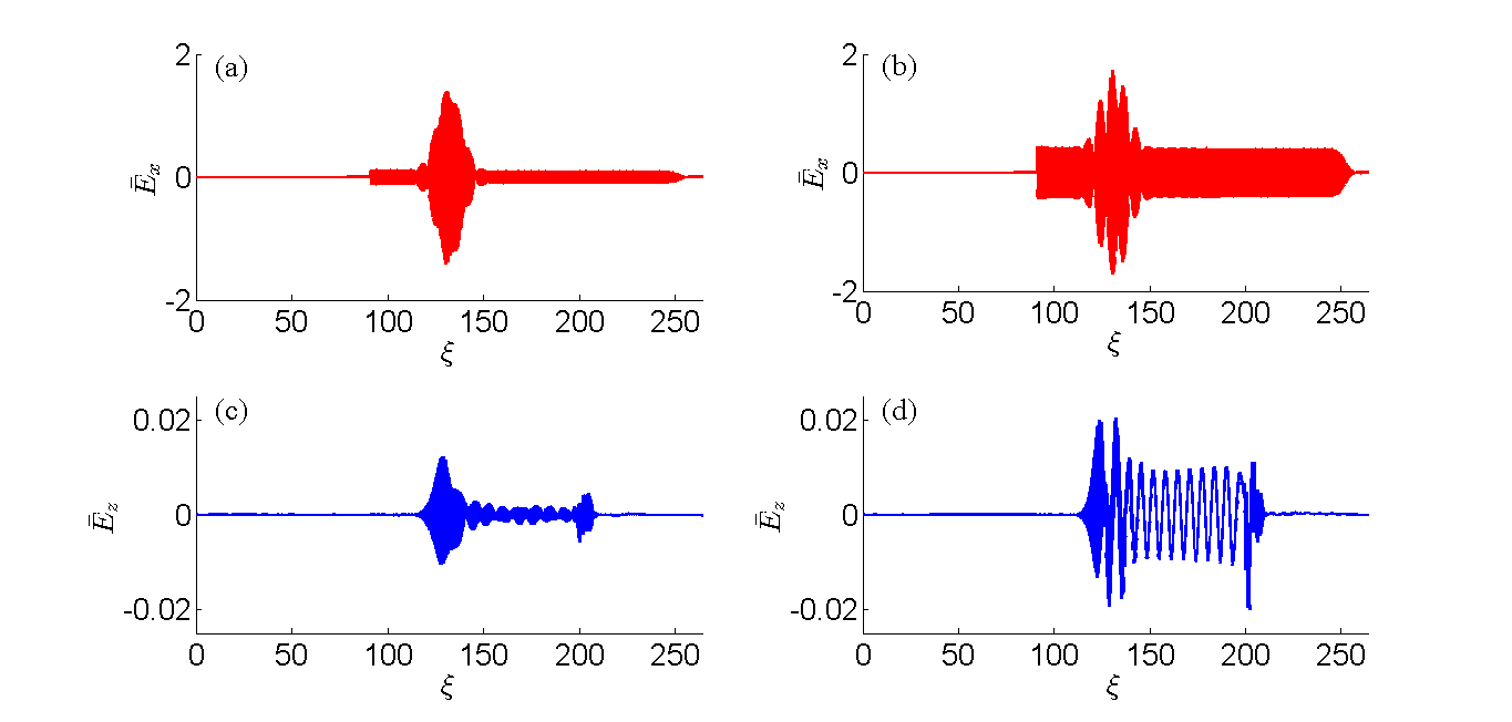
Figure 5: (Color online) The transverse, $\bar{E}_{x}$ (solid line), and longitudinal, $\bar{E}_{z}$ (dashed line), electric fields at $\tau=90$ in the mild, $\bar{v}_{ea}/\bar{v}_{br}=1.5$ (Fig. 5a), and strong, $\bar{v}_{ea}/\bar{v}_{br}=5.5$ (Fig. 5b), wavebreaking regimes.

Figure 6 shows the Fourier-transformed transverse electric field $\bar{E}_{x}$ in these two regimes in $(\hat{k},\hat{\omega})$-space. Fig. 6a shows the mild wavebreaking case of $\bar{v}_{ea}/\bar{v}_{br}=1.5$ and Fig. 6b shows the strong wavebreaking case of $\bar{v}_{ea}/\bar{v}_{br}=5.5$. The spatially Fourier-transformed pump and seed envelopes in the mild wavebreaking regime are shown in Figs. 7a and b. The spatially Fourier-transformed pump and seed envelopes in the strong wavebreaking regime are shown in Figs. 7c and d.

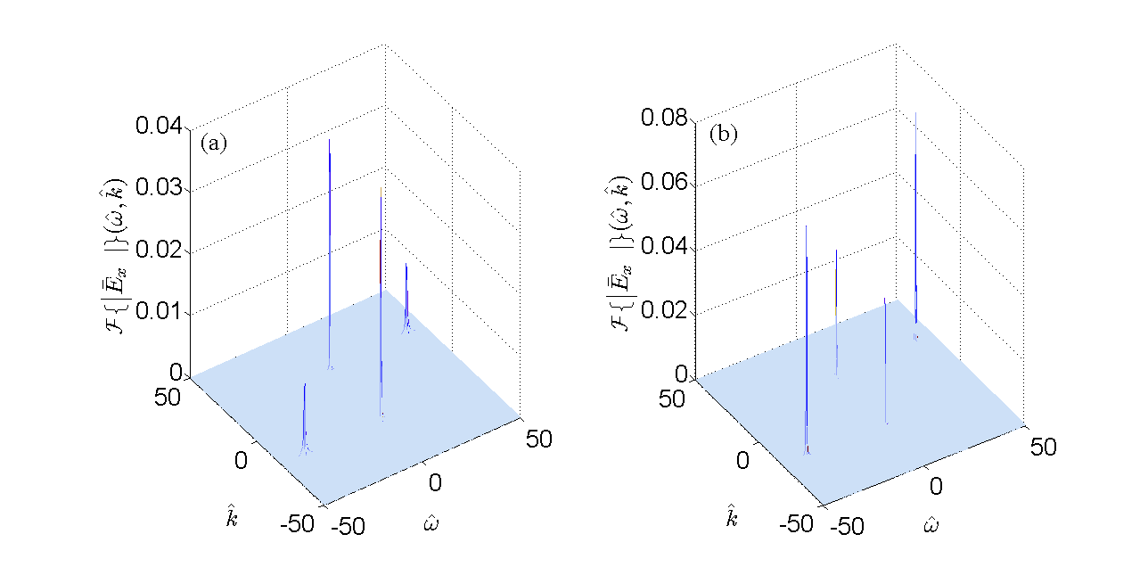
Figure 6: (Color online) The time-space Fourier-transformed transverse field $\bar{E}_{x}$ in the mild wavebreaking regime, $\bar{v}_{ea}/\bar{v}_{br}=1.5$, (Fig. 6a) and in the strong wavebreaking regime, $\bar{v}_{ea}/\bar{v}_{br}=5.5$, (Fig. 6b).

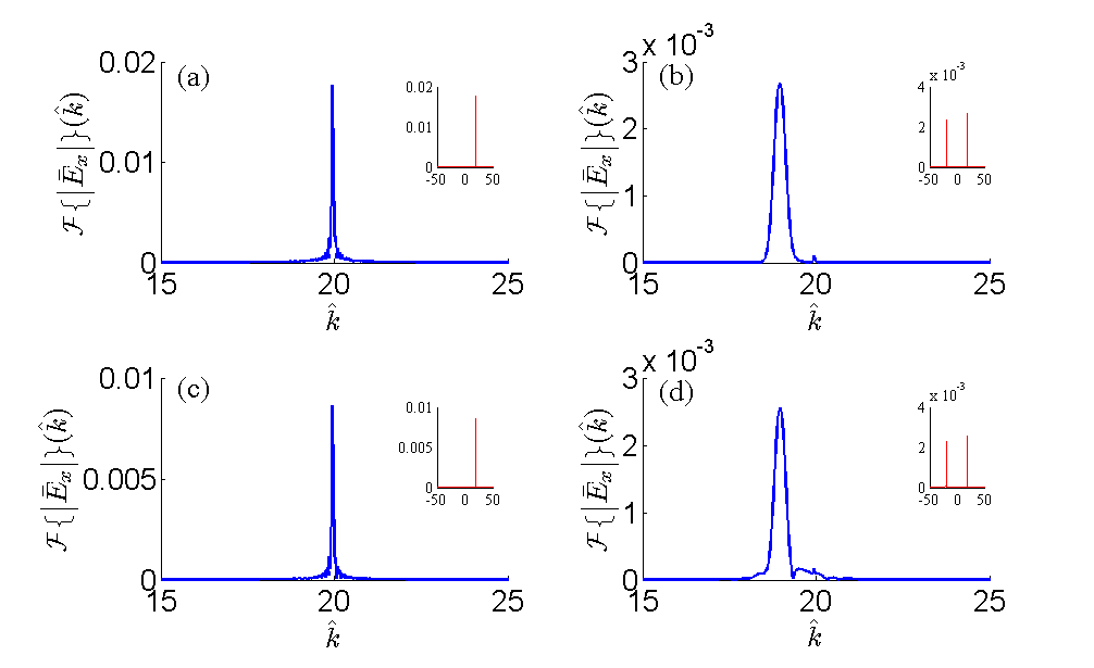
Figure 7: (Color online) The envelope of spatially Fourier-transformed transverse field $\bar{E}_{x}$ in the mild wavebreaking regime, $\bar{v}_{ea}/\bar{v}_{br}=1.5$, at $\hat{\omega}=40$ (Fig. 7a) and $\hat{\omega}=0$ (Fig. 7b). The envelope of spatially Fourier-transformed transverse field $\bar{E}_{x}$ in the strong wavebreaking regime, $\bar{v}_{ea}/\bar{v}_{br}=5.5$, at $\hat{\omega}=40$ (Fig. 7c) and $\hat{\omega}=0$ (Fig. 7d).

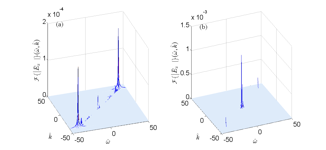
Figure 8: (Color online) The time-space Fourier-transformed longitudinal field $\bar{E}_{z}$ in the mild, $\bar{v}_{ea}/\bar{v}_{br}=1.5$, (Fig. 8a) and strong, $\bar{v}_{ea}/\bar{v}_{br}=5.5$, (Fig. 8b) wavebreaking regimes.

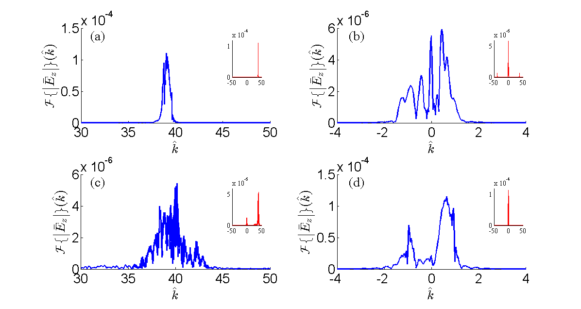
Figure 9: (Color online) The envelope of spatially Fourier-transformed longitudinal field $\bar{E}_{z}$ in the mild wavebreaking regime, $\bar{v}_{ea}/\bar{v}_{br}=1.5$, at $\hat{\omega}=40$ (Fig. 9a) and $\hat{\omega}=0$ (Fig. 9b). The envelop of spatially Fourier-transformed longitudinal field $\bar{E}_{z}$ in the strong wavebreaking regime, $\bar{v}_{ea}/\bar{v}_{br}=5.5$, at $\hat{\omega}=40$ (Fig. 9c) and $\hat{\omega}=0$ (Fig. 9d).

Figure 8 shows the Fourier-transformed longitudinal field $\bar{E}_{z}$ for the mild, $\bar{v}_{ea}/\bar{v}_{br}=1.5$ (Fig. 8a), and strong, $\bar{v}_{ea}/\bar{v}_{br}=5.5$ (Fig. 8b) wavebreaking regimes in $(\hat{k},\hat{\omega})$-space. The spatially Fourier-transformed envelopes of the Langmuir waves associated with the BRA and forward Raman scattering of the seed are shown in Fig. 9. As seen, the bandwidth in the strong wavebreaking regime is broader than in the mild wavebreaking regime. Also, the long-wavelength components located around the spot $(\hat{k},\hat{\omega})=(0,0)$ are much more pronounced in the strong wavebreaking regime.

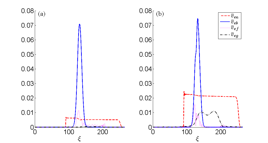
Figure 10: (Color online) Envelopes of electron quiver velocities $\bar{v}_{ea}$, $\bar{v}_{eb}$, $\bar{v}_{ef}$, and $\bar{v}_{eg}$ in the fields of the pump pulse (dashed line), seed pulse (solid line), Langmuir wave mediating BRA (dotted line) and Langmuir wave mediating forward Raman scattering of the seed pulse (dash-dotted line) at $\tau=90$ for $\bar{v}_{ea}/\bar{v}_{br}=1.5$ (Fig. 10a) and $\bar{v}_{ea}/\bar{v}_{br}=5.5$ (Fig. 10b).

Using $(\hat{k},\hat{\omega})$ Fourier images of the fields $\bar{E}_{x}$ and $\bar{E}_{z}$, we calculated the envelopes of the pump pulse, seed pulse, and two Langmuir waves mediating BRA and forward Raman scattering of the seed pulse. Figure 10 shows the results in the mild, $\bar{v}_{ea}/\bar{v}_{br}=1.5$ (Fig. 10a), and strong, $\bar{v}_{ea}/\bar{v}_{br}=5.5$ (Fig. 10b) wavebreaking regimes.

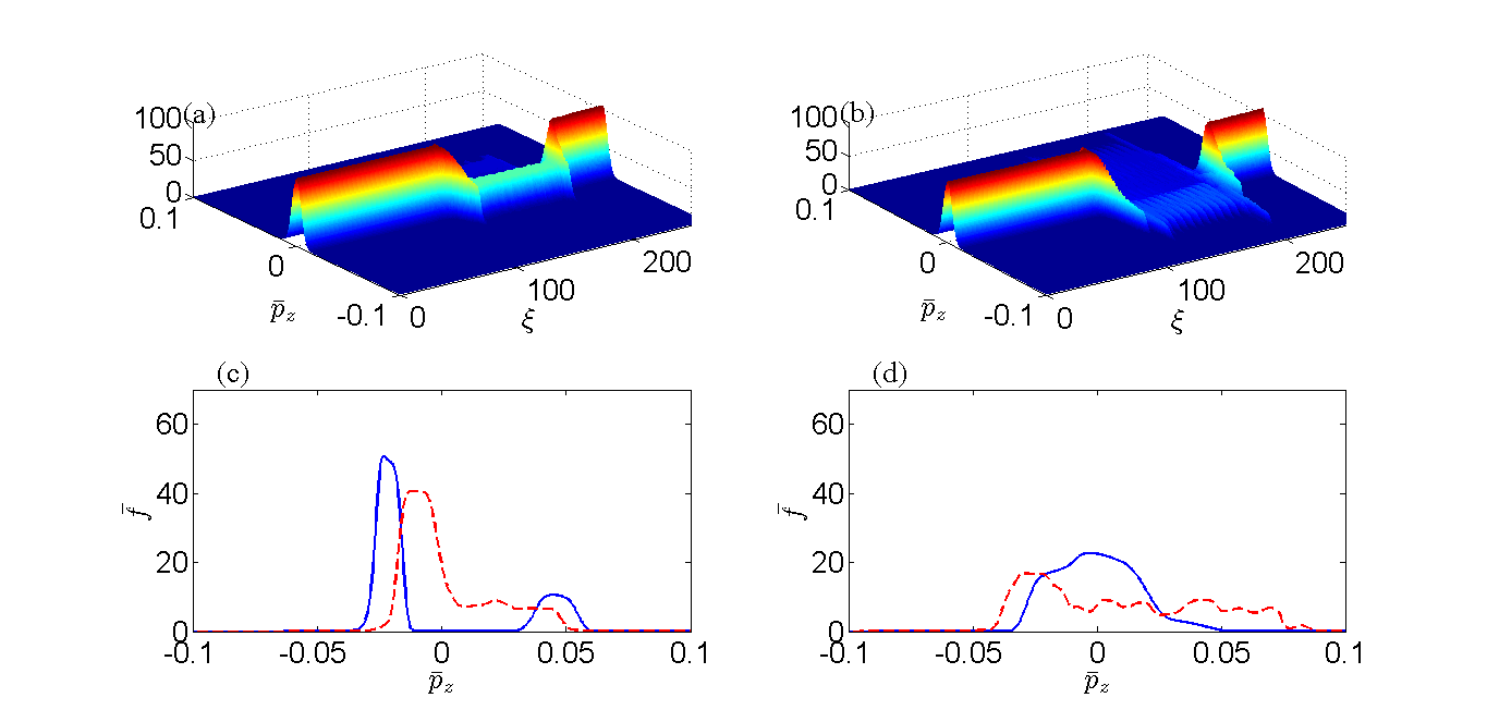
Figure 11: (Color online) The electron distribution function for the mild, $\bar{v}_{ea}/\bar{v}_{br}=1.5$ (Figs. 12a and c), and strong, $\bar{v}_{ea}/\bar{v}_{br}=5.5$ (Figs. 12b and d), wavebreaking regimes. Figs. 12c and d show the distribution snap-shuts at $\xi=132$ (solid line) and $\xi=150$ (dashed line).

Fig. 11 shows the electron distribution function for the mild, $\bar{v}_{ea}/\bar{v}_{br}=1.5$ (Figs. 11a and c), and strong, $\bar{v}_{ea}/\bar{v}_{br}=5.5$ (Figs. 11b and d), wavebreaking regimes. Figs. 11c and d show the distribution snap-shuts at $\xi=132$ (solid line) and $\xi=150$ (dashed line). The effective electron temperatures at $\xi=132$ and $\xi=150$ are $T_{e}=180$ eV and $470$ eV, for the mild wavebreaking regime, and $620$ eV and $870$ eV, for the strong wavebreaking regime, respectively.

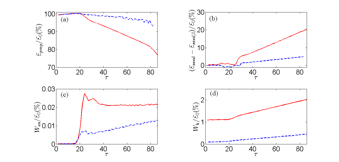
Figure 12: (Color online) Percentage of input pump energy remaining in the pump (Fig. 12a), transferred to the seed (Fig. 12b), electrostatic field (Fig. 12c), and plasma electrons (Fig. 12d) in the mild, $\bar{v}_{ea}/\bar{v}_{br}=1.5$ (solid curve) and strong, $\bar{v}_{ea}/\bar{v}_{br}=5.5$ (dashed curve) wavebreaking regimes.

Finally, Fig. 12 shows the fraction of pump energy that is decayed (a), transferred to the seed (b), to electrostatic waves (c), and to plasma electrons (d), in the mild (solid curve) and strong (dashed curve) wavebreaking regimes. As seen, the pump depletion is significantly larger in the mild wavebreaking regime.

V Discussion

The results obtained here are by and large in agreement with previously reported PIC simulations. However there are also significant discrepancies. In this section, the VM simulations presented here are compared both to previous PIC simulations as well as to theoretical expectations.

This comparison is made in Fig. 13, which shows the relative pump depletion, $\eta$, calculated using our VM code to the results of PIC code simulations  Trines_10 , as well as to the analytical estimate Malkin_99_PRL for the strong wavebreaking regime $\bar{v}_{ea}/\bar{v}_{br}\gg 1$. The solid line is based on our VM simulations at the initial electron temperature $T_{e}=10$ eV and input seed intensity 10 PW$/$cm². The dash-dotted line shows the analytical estimate Malkin_99_PRL , $\eta\sim(\bar{v}_{br}/\bar{v}_{ea})^{2}$. The dashed line is the same estimate with a smaller numerical coefficient, $\eta\sim 0.3\times(\bar{v}_{br}/\bar{v}_{ea})^{2}$. The crosses at $\bar{v}_{br}/\bar{v}_{ea}=0.61$, $1.73$, and $4.88$ show the pump depletion calculated through PIC simulations and reported in Fig. 3a of Ref. Trines_10, . The cross at $\bar{v}_{br}/\bar{v}_{ea}=5.5$ shows the pump depletion reported in Fig. 2a of the same Ref. Trines_10, . Finally, the diamonds show our VM results at larger input seed intensities, 40 PW$/$cm² (the diamond at $\bar{v}_{ea}/\bar{v}_{br}=1.5$) and 100 PW$/$cm² (the diamond at $\bar{v}_{ea}/\bar{v}_{br}=5.5$) .

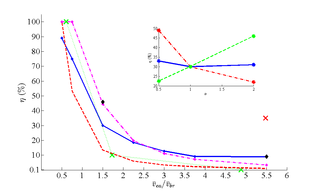
Figure 13: (Color online) The pump depletion calculated numerically using VM code for the initial electron temperature $T_{e}=10$ eV and input seed intensity 10 PW$/$cm² (solid line), the analytical estimate of the Ref.  Malkin_99_PRL, , $\eta\sim(\bar{v}_{br}/\bar{v}_{ea})^{2}$, (dash-dot line), the same estimate with a smaller numerical coefficient, $\eta\sim 0.3\times(\bar{v}_{br}/\bar{v}_{ea})^{2}$ (dashed line); the pump depletion reported in PIC simulations Ref. Trines_10, , Fig. 3a, (crosses at $\bar{v}_{br}/\bar{v}_{ea}=0.61$, $1.73$, and $4.88$) and in the same Ref. Trines_10, , Fig.2a (cross at $\bar{v}_{br}/\bar{v}_{ea}=5.5$). The diamonds show our VM results at larger input seed intensities, 40 PW$/$cm² (the diamond at $\bar{v}_{ea}/\bar{v}_{br}=1.5$) and 100 PW$/$cm² (the diamond at $\bar{v}_{ea}/\bar{v}_{br}=5.5$). The inset shows how the pump depletion depends on the input seed duration and amplitude: the solid line corresponds to constant seed amplitude, the dash-dot line corresponds to constant seed capacity, and the dashed line corresponds to constant seed duration.

It can be seen that the PIC results presented in Fig. 3a of Ref. Trines_10, agree reasonably well both with the analytical estimate of Ref. Malkin_99_PRL, and with our VM simulations. There is somewhat smaller pump depletion in Fig. 3a of Ref. Trines_10, . This might be due to premature backscattering of the pump by PIC noise in the simulations of Ref. Trines_10, . Note that numerical noise would act much like physical noise in inducing premature backscattering. Note also that, although not employed in these simulations, the premature backscattering of the pump by noise, whether physical or numerical noise, could, in principle, be suppressed by selective resonance detuning techniques Malkin_00_PRL ; Malkin_00_POP ; Malkin_14-EPJST . In any event, there is not large discrepancy between results presented in Fig. 3a of Ref. Trines_10, and both our VM simulations and with the analytical estimate.

The large discrepancy occurs in the strong wavebreaking regime case shown in Fig. 2a of Ref. Trines_10, , where the pump intensity is 30 times higher than the wavebreaking threshold ($\bar{v}_{ea}/\bar{v}_{br}=5.5$). Here, the PIC results report a surprisingly high $35\%$ BRA efficiency. This high efficiency disagrees with both our VM numerical simulations results and the analytical estimate of Ref. Malkin_99_PRL, . The high efficiency also appear even to disagree with the efficiency shown in Fig. 3a of the same Ref. Trines_10, . In contrast to the 35% efficiency, the VM simulation, the analytical estimate, and Fig. 3a all give less than $10\%$ pump depletion for such a regime.

The inset of Fig. 13 shows how the pump depletion depends on the input seed duration and amplitude in the mild wavebreaking regime, $\bar{v}_{ea}/\bar{v}_{br}=1.5$. Results for the constant initial seed duration of one plasma period and few input seed amplitudes, marked in the inset of Fig. 13 by few different values of the parameter $\alpha=\bar{v}_{eb}/\bar{v}_{eb,0}$, are shown by the dashed line. Results for constant input seed amplitude, $\bar{v}_{eb}=0.07$, and few input seed durations, marked by few values the parameter $\alpha=\bar{\Delta}_{b}/\bar{\Delta}_{b,0}$, are shown by the solid line. Results for constant seed integrated amplitude $U_{in}=3.5$ and few input seed durations are shown by the dash-dot line. Our results from the inset indicate that in the mild wavebreaking regime it is beneficial to choose high initial seed pulse intensity to obtain maximal BRA efficiency.

VI Summary

The wavebreaking BRA regime in strongly undercritical plasma ($\omega_{a}/\omega_{e}=20$) was studied using a 1D Maxwell-Vlasov code. This code confirmed that efficient BRA is possible for the pump pulse intensities up to a few times larger than the wavebreaking threshold. However, for pump intensities exceeding by more than a factor of 10 the wavebreaking threshold, the amplification efficiency significantly decreases.

For example, for the pump intensity exceeding the wavebreaking threshold by a factor of 30, we only found possible a BRA efficiency of less than $10\%$. This low efficiency is consistent both with the analytical estimate of Ref. Malkin_99_PRL, and with Fig. 3a of Ref. Trines_10, . However, this low efficiency is at variance with Fig. 2a of the same Ref. Trines_10, , where the rather higher efficiency of $35\%$ was reported. It remains of interest, but reserved for a future study, to consider why in fact this difference is so large.

A further important finding of this study is that, in the strong wavebreaking regime, in contrast to the mild wavebreaking regime, increasing the seed pulse intensity does not increase the BRA efficiency.

- (1) D. Strickland and G. Mourou, “Compression of amplified chirped optical pulses,” Opt. Commun. 56, 219 (1985).
- (2) G. A. Mourou, C. P. J. Barty, and M. D. Perry, “Ultrahigh-intensity lasers: physics of the extreme on a tabletop,” Phys. Today 51, 22 (1998).
- (3) I. V. Yakovlev, “Stretchers and compressors for ultra-high power laser systems,” Quantum Electronics 44, 393 (2014).
- (4) V. M. Malkin, G. Shvets, and N. J. Fisch, “Fast compression of laser beams to highly overcritical powers,” Phys. Rev. Lett. 82, 4448 (1999).
- (5) V. M. Malkin, G. Shvets, and N. J. Fisch, “Ultra-powerful compact amplifiers for short laser pulses,” Phys. Plasmas 7, 2232 (2000).
- (6) N. J. Fisch and V. M. Malkin, “Generation of ultrahigh intensity laser pulses,” Phys. Plasmas 10, 2056 (2003).
- (7) V. M. Malkin and N. J. Fisch, “Manipulating ultra-intense laser pulses in plasmas,” Phys. Plasmas 12, 044 507 (2005).
- (8) G. Shvets, N. J. Fisch, A. Pukhov, and J. Meyer-ter-Vehn, “Supperradiant amplification of an ultrashort laser pulse in a plasma by a counterpropagating pump,” Phys. Rev. Lett. 81, 4879 (1998).
- (9) A. A. Andreev, C. Riconda, V. T. Tikhonchuk, and S. Weber, “Short light pulse amplification and compression by stimulated Brillouin scattering in plasmas in the strong coupling regime,” Physics of Plasmas 13, 053 110 (2006).
- (10) L. Lancia, J.-R. Marquès, M. Nakatsutsumi, C. Riconda, S. Weber, S. Hüller, A. Mančić, P. Antici, V. T. Tikhonchuk, A. Héron, P. Audebert, and J. Fuchs, “Experimental Evidence of Short Light Pulse Amplification Using Strong-Coupling Stimulated Brillouin Scattering in the Pump Depletion Regime,” Phys. Rev. Lett. 104, 025 001 (2010).
- (11) S. Weber, C. Riconda, L. Lancia, J.-R. Marquès, G. A. Mourou, and J. Fuchs, “Amplification of Ultrashort Laser Pulses by Brillouin Backscattering in Plasmas,” Phys. Rev. Lett. 111, 055 004 (2013).
- (12) C. Riconda, S. Weber, L. Lancia, J. Marques, G. A. Mourou, and J. Fuchs, “Spectral characteristics of ultra-short laser pulses in plasma amplifiers,” Physics of Plasmas 20, 083 115 (2013).
- (13) V. M. Malkin and N. J. Fisch, “Key plasma parameters for resonant backward Raman amplification in plasma,” Eur. Phys. J. Special Topics 223, 1157 (2014).
- (14) J. M. Dawson, “Nonlinear Electron Oscillations in a Cold Plasma,” Phys. Rev. 113, 383 (1959).
- (15) W. L. Kruer, The Physics of Laser Plasma Interactions (Addison-Wesley, Reading, MA, 1988).
- (16) G. M. Fraiman, N. A. Yampolsky, V. M. Malkin, and N. J. Fisch, “Robustness of laser phase fronts in backward Raman amplifiers,” Phys. Plasmas 9, 3617 (2002).
- (17) V. M. Malkin and N. J. Fisch, “Relic crystal-lattice effects on Raman compression of powerful x-ray pulses in plasmas,” Phys. Rev. Lett. 99, 205 001 (2007).
- (18) V. M. Malkin, Z. Toroker, and N. J. Fisch, “Laser duration and intensity limits in plasma backward Raman amplifiers,” Phys. Plasmas 19, 023 109 (2012).
- (19) G. Lehmann and K. H. Spatschek, “Non-filamentated ultra-intense and ultra-short pulse fronts in three-dimensional Raman seed amplification,” Phys. Plasmas 21, 053 101 (2014).
- (20) V. M. Malkin, G. Shvets, and N. J. Fisch, “Detuned Raman amplification of short laser pulses in plasma,” Phys. Rev. Lett. 84, 1208 (2000).
- (21) V. M. Malkin, Y. A. Tsidulko, and N. J. Fisch, “Stimulated Raman scattering of rapidly amplified short laser pulses,” Phys. Rev. Lett. 85, 4068 (2000).
- (22) A. A. Solodov, V. M. Malkin, and N. J. Fisch, “Pump side scattering in ultrapowerful backward Raman amplifiers,” Phys. Rev. E 69, 066 413 (2004).
- (23) Y. A. Tsidulko, V. M. Malkin, and N. J. Fisch, “Suppression of superluminous precursors in high-power backward Raman amplifiers,” Phys. Rev. Lett. 88, 235 004 (2002).
- (24) A. A. Solodov, V. M. Malkin, and N. J. Fisch, “Random density inhomogeneities and focusability of the output pulses for plasma-based powerful backward Raman amplifiers,” Phys. Plasmas 10, 2540 (2003).
- (25) V. M. Malkin, N. J. Fisch, and J. S. Wurtele, “Compression of powerful x-ray pulses to attosecond durations by stimulated Raman backscattering in plasmas,” Phys. Rev. E 75, 026 404 (2007).
- (26) V. M. Malkin and N. J. Fisch, “Quasitransient regimes of backward Raman amplification of intense x-ray pulses,” Phys. Rev. E 80, 046 409 (2009).
- (27) V. M. Malkin and N. J. Fisch, “Quasitransient backward Raman amplification of powerful laser pulses in plasma with multicharged ions,” Phys. Plasmas 17, 073 109 (2010).
- (28) A. A. Balakin, N. J. Fisch, G. M. Fraiman, V. M. Malkin, and Z. Toroker, “Numerical modeling of quasitransient backward Raman amplification of laser pulses in moderately undercritical plasmas with multicharged ions,” Phys. Plasmas 18, 102 311 (2011).
- (29) M. S. Hur, R. R. Lindberg, A. E. Charman, J. S. Wurtele, and H. Suk, “Electron Kinetic Effects on Raman Backscatter in Plasmas,” Phys. Rev. Lett. 95, 115 003 (2005).
- (30) N. Yampolsky and N. Fisch, “Effect of nonlinear Landau damping in plasma-based backward Raman amplifier,” Phys. Plasmas 16, 072 105 (2009).
- (31) N. Yampolsky and N. Fisch, “Limiting effects on laser compression by resonant backward Raman scattering in modern experiments,” Physics of Plasmas 18, 056 711 (2011).
- (32) D. Strozzi, E. Williams, H. Rose, D. Hinkel, A. Langdon, and J. Banks, “Threshold for electron trapping nonlinearity in Langmuir waves,” Phys. Plasmas 19, 112 306 (2012).
- (33) Z. Wu, Y. Zuo, J. Su, L. Liu, Z. Zhang, and X. Wei, “Production of single pulse by Landau damping for backward Raman amplification in plasma,” IEEE Transactions on Plasma Science 42, 1704–1708 (2014).
- (34) S. Depierreux, V. Yahia, C. Goyon, G. Loisel, P.-E. Masson-Laborde, N. Borisenko, A. Orekhov, O. Rosmej, T. Rienecker, and C. Labaune, “Laser light triggers increased Raman amplification in the regime of nonlinear Landau damping,” Nature Communications 5, 4158 (2014).
- (35) D. S. Clark and N. J. Fisch, “Operating regime for a backward Raman laser amplifier in preformed plasma,” Phys. Plasmas 10, 3363 (2003).
- (36) N. A. Yampolsky, V. M. Malkin, and N. J. Fisch, “Finite-duration seeding effects in powerful backward Raman amplifiers,” Phys. Rev. E 69, 036 401 (2004).
- (37) Z. Toroker, V. M. Malkin, A. A. Balakin, G. M. Fraiman, and N. J. Fisch, “Geometrical constraints on plasma couplers for Raman compression,” Phys. Plasmas 19, 083 110 (2012).
- (38) Z. Toroker, V. M. Malkin, and N. J. Fisch, “Seed Laser Chirping for Enhanced Backward Raman Amplification in Plasmas,” Phys. Rev. Lett. 109, 085 003 (2012).
- (39) Y. Ping, I. Geltner, N. J. Fisch, G. Shvets, and S. Suckewer, “Demonstration of ultrashort laser pulse amplification in plasmas by a counterpropagating pumping beam,” Phys. Rev. E 62, R4532 (2000).
- (40) Y. Ping, I. Geltner, A. Morozov, N. J. Fisch, and S. Suckewer, “Raman amplification of ultrashort laser pulses in microcapillary plasmas,” Phys. Rev. E 66, 046 401 (2002).
- (41) Y. Ping, W. Cheng, S. Suckewer, D. S. Clark, and N. J. Fisch, “Amplification of ultrashort laser pulses by a resonant Raman scheme in a gas-jet plasma,” Phys. Rev. Lett. 92, 175 007 (2004).
- (42) A. A. Balakin, D. V. Kartashov, A. M. Kiselev, S. A. Skobelev, A. N. Stepanov, and G. M. Fraiman, “Laser pulse amplification upon Raman backscattering in plasma produced in dielectric capillaries,” JETP Lett. 80, 12 (2004).
- (43) W. Cheng, Y. Avitzour, Y. Ping, S. Suckewer, N. J. Fisch, M. S. Hur, and J. S. Wurtele, “Reaching the nonlinear regime of Raman amplification of ultrashort laser pulses,” Phys. Rev. Lett. 94, 045 003 (2005).
- (44) J. Ren, S. Li, A. Morozov, S. Suckewer, N. A. Yampolsky, V. M. Malkin, and N. J. Fisch, “A compact double-pass Raman backscattering amplifier/compressor,” Phys. Plasmas 15, 056 702 (2008).
- (45) G. Vieux, A. Lyachev, X. Yang, B. Ersfeld, J. P. Farmer, E. Brunetti, R. C. Issac, G. Raj, G. H. Welsh, S. M. Wiggins, and D. A. Jaroszynski, “Chirped pulse Raman amplification in plasma,” New J. Phys. 13, 063 042 (2011).
- (46) X. Yang, G. Vieux, E. Brunetti, J. P. Farmer, B. Ersfeld, S. M. Wiggins, R. C. Issac, G. H. Welsh, and D. A. Jaroszynski, “Experimental investigation of chirp pulse Raman amplification in plasma,” Proc. SPIE 8075, 80 750G (2011).
- (47) R. M. G. M. Trines, F. Fiuza, R. Bingham, R. A. Fonseca, L. O. Silva, R. A. Cairns, and P. A. Norreys, Nature Phys. 7, 87 (2011).
- (48) P. Bertrand, A. Ghizzo, T. W. Johnston, M. Shoucri, E. Fijalkow, and M. R. Feix, “A nonperiodic Euler-Vlasov code for the numerical simulation of laser-plasma beat wave acceleration and Raman scattering,” Phys. Fluids B 2, 1028 (1990).
- (49) C. Z. Cheng and G. Knorr, “The integration of the Vlasov Equation in Configuration Space,” J. Comp. Phys. 22, 330 (1976).
- (50) T. Reveille, P. Bertrand, A. Ghizzo, J. Lebas, T. W. Johnston, and M. Shoucri, “Stimulated Raman scattering: Close correspondence of Vlasov simulation and coupled modes,” Phys. Fluids B 4, 2665 (1992).
- (51) A. Ghizzo, T. Reveille, P. Bertrand, T. Johntson, J. Lebas, and M. Shoucri, “An Eulerian Vlasov-Hilbert Code for the Numerical-Simulation of the Interaction of High-Frequency Electromagnetic-Waves with Plasma,” J. Comp. Phys. 118, 356–365 (1995).
- (52) J. P. Farmer and A. Pukhov, “Fast multidimensional model for the simulation of Raman amplification in plasma,” Phys. Rev. E 88, 063 104 (2013).
- (53) G. Lehmann, K. H. Spatschek, and G. Sewell, “Pulse shaping during Raman-seed amplification for short laser pulses,” Phys. Rev. E 87, 063 107 (2013).
- (54) J.-P. Berenger, “A Perfectly Matched Layer for the Absorption of Electromagnetic Waves,” J. Comp. Phys. 114, 185–200 (1994).
- (55) S. D. Gedney, “An Anisotropic Perefectly Matched Layer-Absorbing Medium for the Truncation of FDTD Lattices,” IEEE Trans. Antennas Propag. 44, 1630 (1996).
- (56) E. P. Gross and M. Krook, “Model for Collision Processes in Gases: Small-Amplitude Oscillations of Charged Two-Component Systems,” Phys. Rev. 102, 593–604 (1956).
- (57) E. Bedrosian, “A Product Theorem for Hilbert Transforms,” Rand Corporation Memorandum (RM-3439-PR) (1962).