Gravitational waves from the evolution of magnetic field after electroweak epoch

Abstract

It was recently demonstrated that the evolution of helical magnetic field in the primordial plasma at temperatures $T\gtrsim 10$ MeV is affected by the phenomenon of chiral quantum anomaly in the electroweak model, leading to a possibility of self-sustained existence of magnetic field and chiral asymmetry in the electronic distribution. This may serve as a mechanism for generating primordial magnetic field in the early universe. Violent magnetic-field generation may lead to production of gravitational waves which, regardless of the fate of magnetic field itself, survive until today. We estimate the threshold value of the initial chiral asymmetry above which the generated gravitational waves would affect the big-bang nucleosynthesis and would show up in the current and future experiments on gravitational-wave detection.

1 Introduction

Observations have established the omnipresence of magnetic field in the universe of various magnitudes and on various spatial scales. Galaxies such as Milky Wave possess regular magnetic fields of the order of $\mu$G, and coherent fields of the order of $100~{}\mu$G are detected in distant galaxies [1, 2]. Recently, an evidence was obtained for the presence of magnetic field in intergalactic medium, including voids [3, 4, 5], with strengths exceeding $\sim 10^{-15}$ G. This supports the idea of cosmological origin of magnetic fields, which are subsequently amplified in galaxies, probably by the dynamo mechanism (see a review in [6]).

The origin of cosmological magnetic field is a problem yet to be solved, while there exist several mechanisms by which this could be achieved. They can broadly be classified into inflationary and post-inflationary scenarios. Both types still face problems to overcome: inflationary magnetic fields usually turn out to be rather weak, while those produced after inflation typically have too small coherence lengths (see [6, 7] for a review of these mechanisms and assessment of these difficulties). There is a hope that these problems can be solved by taking into account some additional mechanisms; for instance, the coherence length can be increased by the so-called ‘inverse cascade’ in turbulent hydrodynamics, which transfers power and energy from short to long spatial scales.

One of the mechanisms of generation of cosmological magnetic fields which is currently under scrutiny is based on the chiral (axial) quantum anomaly present in the theory of electroweak interactions [8]. If the numbers of right-handed and left-handed electrons in the early hot universe happen to deviate from their equilibrium values (for example, due to leptogenesis involving physics beyond the standard model), so that the corresponding non-equilibrium effective chemical potentials $\mu_{\rm L}$ and $\mu_{\rm R}$ differ from each other, then a specific instability arises with respect to generation of helical (hypercharge) magnetic field. The generated helical magnetic field, in turn, is capable of supporting the electron chiral asymmetry, thus prolonging its own existence to cosmological temperatures as low as tens of MeV [9].

The processes of magnetic-field generation such as the one just described will be accompanied by production of gravitational waves. One of the consistency checks for such scenarios is provided by the experimental upper bounds on the gravitational-wave background. In this paper, we would like to address this issue to determine the gravitational-wave background and to see whether it places any constraints on the mechanism discussed above.

We consider magnetic field generated in the early hot universe on electroweak temperature scale $T_{\rm in}\sim 100$ GeV. As mentioned above, such a field can be sustained by quantum anomaly until much lower temperatures of the order of 10 MeV, with power being permanently transformed from short to long spatial scales (the so-called ‘inverse cascade’). It turns out that the whole process of magnetic-field evolution leads to gravitational-wave production which is very sensitive to the characteristics of the initial spectrum of the magnetic field, in particular, exponentially depends on the magnitude of the initial chiral asymmetry. One of the aims of this paper is to determine the threshold for this latter quantity above which the generated gravitational waves would affect the big-bang nucleosynthesis and would be detectable in the current and future experiments on gravitational-wave detection. We will see that such a threshold for the conformal difference of chemical potentials $\Delta\mu_{c}=a(\mu_{\rm L}-\mu_{\rm R})$ at $T_{\rm in}\simeq 100$ GeV is of the order $\Delta\mu_{0}\sim 10^{-4}$.

The paper is organized as follows. In Sec. 2, we describe the spectra of the helical magnetic fields; in Sec. 3, we introduce the basic parameter of the theory under consideration and present the main equations describing the generation of gravitational waves by evolving magnetic fields; in Sec. 4, we give the constraints on the initial energy density in magnetic field, stemming from non-detection of the produced gravitational waves or from the theory of big-bang nucleosynthesis and recombination, under the assumption of the initial value of chiral asymmetry $\Delta\mu_{0}=6\times 10^{-5}$, which was adopted in [9], and demonstrate that the level of the produced gravitational radiation is practically negligible in this case; in Sec. 5, we determine the threshold of the quantity $\Delta\mu_{0}$ (which turns out to be of the order of $10^{-4}$), above which the generated gravitational waves would affect the big-bang nucleosynthesis and would be detectable in the current and future experiments on gravitational waves; in Sec 6, we formulate our conclusions. Technical details on the theory of generation of gravitational waves are presented in Appendix A; the power spectrum of the generated gravitational waves is calculated in Appendix B; the simple case of a monochromatic magnetic field is considered in Appendix C.

2 Helical magnetic fields

The source of gravitational waves is the stress tensor of matter. In the flat space-time, the stress tensor of dissipationless magnetohydrodynamics (MHD) is given by [10]

$$T_{ij}=\rho v_{i}v_{j}+p\delta_{ij}-\left(B_{i}B_{j}-\frac{1}{2}\delta_{ij}B^{2}\right)\,,$$ (2.1)

where $v_{i}$ is the fluid velocity, $p$ is pressure, and $B_{i}$ is the magnetic field. During the epoch of gravitational-wave production under consideration in this paper, the electric conductivity $\sigma$ of the cosmological plasma is very large, so that electric field can be neglected. Only the fluid velocity and magnetic field contribute to the traceless part, relevant to the production of gravitational waves (see Appendix A).

In this paper, we concentrate on the magnetic part of the stress tensor, which we assume to be the major contribution to the gravitational-wave production. The role of turbulence in the process of magnetic field generation was under consideration, e.g., in [11, 12].

In an expanding universe, it is convenient to work in the comoving conformal coordinate system $(\tau,{\boldsymbol{x}})$, in which the magnetic part of the stress tensor (2.1) takes the form

$$T_{ij}=-\frac{1}{a^{2}}\left(B_{i}B_{j}-\frac{1}{2}\delta_{ij}B^{2}\right)\,,$$ (2.2)

where $a(\tau)$ is the scale factor.

A generic two-point correlation function for a divergence-free statistically homogeneous and isotropic magnetic field in Fourier representation has the form [13]

$$\left\langle B_{i}({\boldsymbol{k}})B_{j}^{*}({\boldsymbol{k}}^{\prime})\right\rangle=\left(2\pi\right)^{3}\delta\left({\boldsymbol{k}}-{\boldsymbol{k}}^{\prime}\right)\left[P_{ij}({\boldsymbol{k}})S(k)+i\epsilon_{ijs}\hat{k}^{s}A(k)\right]\,,$$ (2.3)

where $\hat{k}^{i}=k^{i}/k$, $P_{ij}=\delta_{ij}-\hat{k}_{i}\hat{k}_{j}$ is the symmetric projector to the plane orthogonal to ${\boldsymbol{k}}$, and $\epsilon_{ijk}$ is the normalized totally antisymmetric tensor.

It is useful to introduce the helicity components $B_{\pm}({\boldsymbol{k}})$ of the magnetic field via

$$B_{i}({\boldsymbol{k}})=B_{+}({\boldsymbol{k}}){\rm e}^{+}_{i}({\boldsymbol{k}})+B_{-}({\boldsymbol{k}}){\rm e}^{-}_{i}({\boldsymbol{k}})\,,$$ (2.4)

where the basis ${\rm e}^{\pm}_{i}=\frac{1}{\sqrt{2}}\left({\rm e}^{1}_{i}\pm i{\rm e}^{2}_{i}\right)$ is formed from a right-handed orthonormal (with respect to the metric $\delta_{ij}$) basis ${\bf e}^{1}({\boldsymbol{k}})$, ${\bf e}^{2}({\boldsymbol{k}})$, ${\bf e}^{3}({\boldsymbol{k}})={\boldsymbol{k}}/k$. The symmetric and helical parts of the correlation function are then expressed through these components as follows:

$$S(k) = \frac{1}{2}\left\langle|B_{-}({\boldsymbol{k}})|^{2}+|B_{+}({\boldsymbol{k}})|^{2}\right\rangle\,,$$ (2.5)

$$A(k) = \frac{1}{2}\left\langle|B_{-}({\boldsymbol{k}})|^{2}-|B_{+}({\boldsymbol{k}})|^{2}\right\rangle\,.$$ (2.6)

We note an obvious constraint $|A(k)|\leq S(k)$.

The helical part $A(k)$ of the magnetic-field correlation function characterizes the difference in the power between the left-handed and right-handed magnetic field. The symmetric part $S(k)$ characterizes the magnetic field energy density. Magnetic field can be dominated by its left-handed or right-handed part. In this case, of the so-called maximally helical magnetic field, one has $|A(k)|=S(k)$.

Of relevance to the investigation in the present paper will be the case where the right-handed and left-handed magnetic-field components evolve separately as

$$B_{\pm}({\boldsymbol{k}},\tau)=B_{\pm}({\boldsymbol{k}})g_{\pm}(k,\tau)\,,$$ (2.7)

where $B_{\pm}({\boldsymbol{k}})$ are the initial values of the field components at some moment of time, and $g_{\pm}(k,\tau)$ are the corresponding growth factors. In this case, we can work in the random-phase approximation for the initial field, thinking of the initial amplitudes $|B_{\pm}({\boldsymbol{k}})|$ as specified by the spectral functions $S(k)$ and $A(k)$ via (2.5) and (2.6), and of their phases as of random and independent for different ${\boldsymbol{k}}$. In this case, the definitions of the correlation function (2.3) and relations (2.5) and (2.6) are preserved with time, and the spectral functions evolve as follows:

$$\begin{array}[]{l}S(k,\tau)=S(k)f_{+}(k,\tau)+A(k)f_{-}(k,\tau)\,,\vskip 6.0pt plus 2.0pt minus 2.0pt\\ A(k,\tau)=A(k)f_{+}(k,\tau)+S(k)f_{-}(k,\tau)\,.\end{array}$$ (2.8)

where

$$f_{\pm}(k,\tau)=\frac{|g_{-}(k,\tau)|^{2}\pm|g_{+}(k,\tau)|^{2}}{2}\,.$$ (2.9)

This “random-phase” approximation allows us to use the Wick’s theorem for the four-point correlation function.

If the mechanism of generation of magnetic field is local and causal, as will be assumed in the present paper, then the magnetic-field power tends to zero as $k\to 0$ due to the analyticity requirements. Indeed, the Taylor expansion of the spectrum at small $k$ then has the form $S(k)\sim k^{n}$ with the condition $n\geq 2$ stemming from the property of the correlation function having compact support [13].

3 Gravitational waves from helical magnetic fields

According to the scenario proposed and described in [8, 9], a configuration of maximally helical (hypercharge) magnetic field rapidly develops before the electroweak phase transition in the presence of the electron chiral asymmetry due to the effect of axial anomaly. Supported by the electron chiral asymmetry, magnetic field can survive down to cosmological temperatures of the order of 10 MeV, after which the effects of chirality flips and plasma conductivity become more efficient.

Depending on the sign of leptonic chiral asymmetry, one of the helicity components of magnetic field gets amplified due to a specific instability, while the opposite helicity component gets suppressed and can be neglected. The correlation function of a maximally helical magnetic field is then characterized by a single quantity $S(k)$ by virtue of (2.5) and (2.6). For definiteness, we will assume that the amplified component is left-handed.

The evolution factor for the left-handed magnetic field in (2.7) is given by the expression [9]

$$g_{-}({\boldsymbol{k}},\tau)\equiv g_{k}(\tau)=e^{-{\cal A}(\tau)k^{2}+{\cal B}(\tau)k}\,,$$ (3.1)

with the following dimensionless coefficients of the powers of $k$:

$${\cal A}(\tau)=\frac{\tau-\tau_{\rm in}}{\sigma_{c}}\,,\qquad{\cal B}(\tau)=\frac{\alpha}{2\pi\sigma_{c}}\int^{\tau}_{\tau_{\rm in}}\Delta\mu_{c}(\tau^{\prime})d\tau^{\prime}\,.$$ (3.2)

Here, $\sigma_{c}\equiv a\sigma={\rm const}$ [14] characterizes the plasma conductivity, $\alpha\approx 1/137$ is the fine structure constant, and $\Delta\mu_{c}\equiv a\left(\mu_{L}-\mu_{R}\right)$ is the (conformal) difference between the chemical potentials of the left-handed and right-handed charged leptons. This last quantity, in the presence of a maximally helical magnetic field, evolves according to the system of equations [8, 9]

$$\Delta\dot{\mu}_{c}(\tau) = -\frac{c_{\Delta}\alpha}{\pi^{2}}\int_{0}^{\infty}\dot{S}(\tau,k)kdk-\Gamma_{\rm f}(\tau)\Delta\mu_{c}(\tau)\,,$$ (3.3)

$$\dot{S}(\tau,k) = \left(-\frac{2k^{2}}{\sigma_{c}}+\frac{\alpha k\Delta\mu_{c}}{\pi\sigma_{c}}\right)S(\tau,k)\,,$$ (3.4)

where $c_{\Delta}$ is a numerical factor of order unity, and $\Gamma_{\rm f}(\tau)$ is the (time-dependent) rate of chirality flipping due to scattering processes.

As a characteristic example, one can consider a scenario [9] where, due to the growth instability described by (3.1), the magnetic field on a short time scale $\tau\sim\tau_{\rm in}$ develops a maximally helical state with spectrum of the form

$$S(k)=S_{0}\left(\frac{k}{k_{0}}\right)^{2}e^{-k^{2}/k_{0}^{2}}\,,$$ (3.5)

which is analytic at $k=0$ and has a cut-off at the scale $k_{0}$. Then, neglecting the last (flipping) term in (3.3), we see that there is an initial stable point

$$\Delta\mu_{0}=\frac{3\pi k_{0}}{\alpha}\,,$$ (3.6)

at which one initially has $\Delta\dot{\mu}_{c}=0$.

With the flipping term in (3.3) taken into account, a typical law of the evolution of the difference between the chemical potentials can be approximated by the power law [9]

$$\Delta\mu_{c}(\tau)=\Delta\mu_{0}\left(\frac{\tau}{\tau_{\rm in}}\right)^{-\beta}\,,$$ (3.7)

in which $\Delta\mu_{0}$ is given by (3.6). The evolution in the form (3.7) proceeds until the temperature drops to about $T\sim 10$ MeV at the corresponding time $\tau_{\rm fin}$, after which this quantity rapidly decays as a consequence of dissipation. The spectral density of magnetic field during this period evolves according to (3.1).

In a radiation-dominated early universe, it is convenient to choose the scale factor as the inverse of the temperature, $a=1/T$, since the product $aT$ is constant as long as the number of relativistic degrees of freedom $g_{*}$ in the universe remains constant. With this choice, we have $a=\tau/M_{*}$, where $M_{*}=\left(45/4\pi^{3}g_{*}\right)^{1/2}M_{\rm P}$ is the effective Planck mass. Then the relative plasma conductivity $\sigma_{c}=\sigma/T\simeq 70$ [14], the initial conformal time $\tau_{\rm in}=M_{*}/T_{\rm in}\simeq 7.3\times 10^{15}\left(100~{}{\rm GeV}/T_{\rm in}\right)$, and the final conformal time $\tau_{\rm fin}=M_{*}/T_{\rm fin}\simeq 1.5\times 10^{19}\left(50~{}{\rm MeV}/T_{\rm fin}\right)$ with $g_{*}\approx 100$.

If we take the quantities $S_{0}$ and $\Delta\mu_{0}$ as our basic parameters in the initial spectrum of magnetic field, then the cutoff wave number $k_{0}$ in (3.5) is determined from the value of $\Delta\mu_{0}$ via (3.6). For instance, for a characteristic value $\Delta\mu_{0}=6\times 10^{-5}$, we have $k_{0}=4.6\times 10^{-8}$. In this case, the exponent $\beta\simeq 0.35$ according to the numerical simulations of [9]. All our estimates below will refer to the case of $\Delta\mu_{0}=6\times 10^{-5}$, $T_{\rm in}\simeq 100$ GeV and $T_{\rm fin}\sim 50$ MeV.

The wave number $k_{m}$ that maximizes the value of $g_{k}(\tau)$ in (3.1) decreases monotonically from $k_{m}=0.75k_{0}$ at $\tau=\tau_{\rm in}$ to $k_{m}=0.08k_{0}$ at $\tau=\tau_{\rm fin}$. For our typical values $T_{\rm in}\simeq 100$ GeV and $T_{\rm fin}\simeq 50$ MeV, the exponent in $g_{k_{m}}(\tau)$ increases monotonically from zero to $4.2\times 10^{15}k_{0}^{2}\approx 9$ for $\Delta\mu_{0}=6\times 10^{-5}$, leading to a considerable amplification of the initial magnetic field at large spatial scales and to an ‘inverse-cascade’ reddening of its spectrum.

Due to our choice of the scale factor as the inverse temperature, the initial magnetic energy density is given by the expression

$$\rho_{B}(\tau_{\rm in})=\frac{T_{\rm in}^{4}}{2\pi^{2}}\int_{0}^{\infty}S(k)k^{2}dk=\frac{3S_{0}k_{0}^{3}}{16\pi^{3/2}}T_{\rm in}^{4}\,.$$ (3.8)

It is convenient to relate this quantity to the radiation energy density by introducing the dimensionless parameter

$$r_{B}\equiv\frac{\rho_{B}(\tau_{\rm in})}{\rho_{r}(\tau_{\rm in})}=\frac{30\rho_{B}}{\pi^{2}g_{*}T_{\rm in}^{4}}=\frac{15}{\pi^{4}g_{*}}\int_{0}^{\infty}S(k)k^{2}dk=\frac{90S_{0}k_{0}^{3}}{16\pi^{7/2}g_{*}}\,.$$ (3.9)

When making estimates, we will always assume this parameter to be smaller than unity, which simply means that the energy density of magnetic field does not exceed the energy density of radiation in the hot universe.

The details of the derivation of the produced gravitational radiation in the scenario under consideration are presented in Appendices A and B. The energy density of gravitational waves $\rho_{\rm gw}$ is proportional to the square of the initial amplitude $S_{0}$ of the magnetic-field spectral density. Therefore, it is convenient to introduce a normalized dimensionless quantity which is independent of this amplitude:

$$\Upsilon_{\rm gw}=\frac{\rho_{\rm gw}}{r^{2}_{B}\rho_{r}}\left[\frac{g_{*}}{g(\tau)}\right]^{1/3}=\frac{\Omega_{\rm gw}(\tau)}{r^{2}_{B}\Omega_{r}(\tau)}\left[\frac{g_{*}}{g(\tau)}\right]^{1/3}\,,$$ (3.10)

where $\Omega_{\rm gw}(\tau)$ and $\Omega_{r}(\tau)$ are the time-dependent fractions of the energy density in gravitational waves and in radiation, respectively, and $g(\tau)$ is the effective number of the degrees of freedom in radiation, initially equal to $g_{*}$. This quantity has a natural spectral decomposition

$$\Upsilon_{\rm gw}=\int\Upsilon_{q}\,d\ln q\,,$$ (3.11)

where the quantity $\Upsilon_{q}$ determines the spectral power of gravitational waves per logarithmic frequency interval. Note that the quantity $\Upsilon_{q}$ is defined only for wave numbers $q$ inside the Hubble radius, i.e., for $q\tau>1$. The energy density of free gravitational waves evolves with time as $a^{-4}$. As a consequence of entropy conservation, the energy density of radiation evolves as $g^{-1/3}a^{-4}$. Therefore, the quantity $\Upsilon_{q}$ remains constant in time.

The effect of the inverse-cascade modification of the magnetic-field power spectrum by the evolution factor (3.1) on the production of gravitational waves is calculated in Appendix B. It depends on the main parameters of the evolution of magnetic field. For sufficiently large values of $q$, namely, for

$$q\tau_{\rm in}\gtrsim\left(\frac{9k_{0}^{2}\tau_{\rm in}}{16\sigma_{c}}\right)^{1/(1-2\beta)}\,,$$ (3.12)

the quantity $\Upsilon_{q}$ can be approximated by the analytic formula

$$\Upsilon_{q} \simeq \left(\frac{q}{k_{0}}\right)^{3}\left[\ln^{2}\left(1+\frac{1}{q\tau_{\rm in}}\right)\left(1+\frac{q^{2}}{k_{0}^{2}}\right)\phantom{\left(\frac{\tau_{\rm fin}}{\tau_{\rm in}}\right)^{2\beta}}\right.$$ (3.13)

$$\left.{}+R\ln^{2}\left(1+\frac{1}{q\tau_{\rm fin}}\right)\left(1+\left(\frac{\tau_{\rm fin}}{\tau_{\rm in}}\right)^{2\beta}\frac{q^{2}}{k_{0}^{2}}\right)e^{-2{\cal A}_{\rm fin}q^{2}}\right]e^{-q^{2}/k_{0}^{2}}\,,$$

where the quantity $R$ is given by (B):

$$R=\frac{6}{k_{0}}\sqrt{\frac{\sigma_{c}}{\tau_{\rm fin}}}\left(\frac{\tau_{\rm in}}{\tau_{\rm fin}}\right)^{2+6\beta}\exp\left[{\frac{9k_{0}^{2}\tau_{\rm fin}}{4(1-\beta)^{2}\sigma_{c}}\left(\frac{\tau_{\rm in}}{\tau_{\rm fin}}\right)^{2\beta}}\right]\,.$$ (3.14)

For small values of $q$, opposite to (3.12), it is approximated by (3.13) with $R=0$ :

$$\Upsilon_{q}\simeq\left(\frac{q}{k_{0}}\right)^{3}\left(1+\frac{q^{2}}{k_{0}^{2}}\right)\ln^{2}\left(1+\frac{1}{q\tau_{\rm in}}\right)e^{-q^{2}/k_{0}^{2}}\,.$$ (3.15)

The term with $R$ in (3.13) is shown in Appendix B to be insignificant under the characteristic model parameters $T_{\rm in}\simeq 100~{}{\rm GeV}$, $T_{\rm fin}\simeq 50~{}{\rm MeV}$, and $\Delta\mu_{0}=6\times 10^{-5}$, studied in [9]. The quantity $\Upsilon_{q}$ in this case is approximated by (3.15). This function is plotted in Fig. 1 for the specified evolution of magnetic field (3.1)–(3.7) with $k_{0}=4.6\times 10^{-8}$, corresponding to $\Delta\mu_{0}=6\times 10^{-5}$. The spectrum of gravitational waves rises at small wavenumbers and is exponentially suppressed at large wavenumbers characteristic of the similar suppression in the magnetic-field power spectrum, i.e., at $q\sim k_{0}$.

By integrating over all wave numbers, we find

$$\Upsilon_{\rm gw}\simeq\frac{1}{k_{0}^{2}\tau_{\rm in}^{2}}\simeq 10^{-17}\,,$$ (3.16)

where the numerical estimate is made for the parameter values in the scenario under consideration.

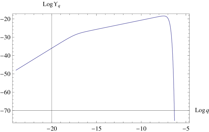
Figure 1: The quantity $\log_{10}\Upsilon_{q}$ versus $\log_{10}q$ as given by equation (3.15) for the parameter values of the evolution of magnetic field described in Sec. 3.

4 The background of gravitational waves

In this section, we calculate the background of gravitational waves depending on the parameter $r_{B}$ of magnetic field defined in (3.9) and assuming the characteristic model parameters $T_{\rm in}\simeq 100~{}{\rm GeV}$, $T_{\rm fin}\simeq 50~{}{\rm MeV}$, $\Delta\mu_{0}=6\times 10^{-5}$, studied in [9].

To compare our calculations of the gravitational-wave background with various constraints, we express our results in conventional notation. The frequency $f$ of gravitational waves today is related to its physical wavelength $\lambda_{\rm phys}$, physical wave number $q_{\rm phys}$, and comoving wave number $q$ by the relations

$$f=\frac{1}{\lambda_{\rm phys}}=\frac{q_{\rm phys}}{2\pi}=\frac{qT_{0}}{2\pi\hbar}\left(\frac{2}{g_{*}}\right)^{1/3}\,,$$ (4.1)

where $T_{0}$ is the current temperature of the CMB.

The spectral energy density of the gravitational waves generated at a radiation-dominated stage is expressed through $\Upsilon_{q}$ as

$$\Omega_{\rm gw}(f)\equiv\frac{8\pi G}{3H^{2}}\frac{d\rho_{\rm gw}}{d\ln f}=r^{2}_{B}\Omega_{r}\left[\frac{g(\tau)}{g_{*}}\right]^{1/3}\Upsilon_{q}\,.$$ (4.2)

The quantities $q$ and $f$ in (4.2) are related with each other through Eq. (4.1).

Note that the comoving wave number associated with the Hubble radius for a radiation-dominated universe ($\ell_{H}=1/H$) is given by

$$q_{H}=\frac{2\pi a}{\ell_{H}}=\frac{2\pi}{\ell_{H}T}\left[\frac{g_{*}}{g(\tau)}\right]^{1/3}=\frac{2\pi T}{M_{*}}\left[\frac{g(\tau)}{g_{*}}\right]^{1/6}\simeq 10^{-17}\left(\frac{g_{*}}{100}\right)^{1/2}\left[\frac{g(\tau)}{g_{*}}\right]^{1/6}T_{\rm GeV}\,,$$ (4.3)

where $T_{\rm GeV}$ is the numerical value of the temperature in GeV.

We compare the results of the gravitational-wave background in the scenario under consideration with a number of constraints — stemming from the BBN prediction of the abundance of light elements, the CMB temperature anisotropy, and the pulsar timing arrays — and with the sensitivity limits of the current and future experiments on direct gravitational-wave detection (LIGO, LISA, and BBO).

4.1 The BBN constraint

The energy density $\rho_{\rm rel}$ of relativistic matter other than photons in the early universe is encoded in the effective number of neutrino species $N_{\nu}$ :

$$\frac{\rho_{\rm rel}}{\rho_{\gamma}}=\frac{7}{8}N_{\nu}\,.$$ (4.4)

The BBN constraints on the quantity $N_{\nu}$ are ranging from $3.04$ to about 5 [15]. The measurements of the light-element abundances combined with the analysis of the Wilkinson Microwave Anisotropy Probe (WMAP) data [16] give the constraint $2.67<N_{\nu}<3.65$ at 68% CL.

Gravitational waves are among the relativistic components in (4.4), which leads to upper bounds on their energy density. According to (4.3), the comoving wave number associated with the Hubble radius at that time is equal to $q_{\rm NS}\simeq 5\times 10^{-22}$, which is very small. Thus, we can use equations (3.10) and (3.16) to obtain the level of gravitational waves during the epoch of nucleosynthesis:

$$\frac{\rho_{\rm gw}}{\rho_{\gamma}}=\frac{\rho_{\rm gw}}{\rho_{r}}\frac{\rho_{r}}{\rho_{\gamma}}=r_{B}^{2}\Upsilon_{\rm gw}\left(\frac{g}{g_{*}}\right)^{1/3}\frac{g}{2}\simeq 4.8\times 10^{-18}r_{B}^{2}\,,$$ (4.5)

where we have substituted $g=3.36$ and $g_{*}=100$. For the natural upper bound $r_{B}<1$ (in typical scenarios, we have [9] $r_{B}<10^{-5}$), the BBN constraint is satisfied with a huge margin.

4.2 The CMB constraint

The Cosmic Bakground Explorer (COBE) measurements give the today’s energy density constraint [17]

$$h^{2}\Omega_{\rm gw}(f)<7\times 10^{-11}\left(\frac{H_{0}}{f}\right)^{2}$$ (4.6)

on gravitational waves in the frequency region $f\in[3\times 10^{-18},10^{-16}]$ Hz. In particular, we have

$$\begin{array}[]{ll}h^{2}\Omega_{\rm gw}(f)<7.4\times 10^{-14}\,,&f=10^{-16}~{}\mbox{Hz}\,,\vskip 6.0pt plus 2.0pt minus 2.0pt\\ h^{2}\Omega_{\rm gw}(f)<8.2\times 10^{-11}\,,&f=3\times 10^{-18}~{}\mbox{Hz}\,.\end{array}$$ (4.7)

The relevant region of comoving wave numbers, according to (4.1), is $q\in[2\times 10^{-28},\,6.5\times 10^{-27}]$. Using (4.2) and (3.15) and taking into account that today $\Omega_{r}\simeq 4\times 10^{-5}$, we obtain

$$\begin{array}[]{ll}h^{2}\Omega_{\rm gw}(f)\sim 9\times 10^{-60}r^{2}_{B}\,,&f=10^{-16}~{}\mbox{Hz}\,,\vskip 6.0pt plus 2.0pt minus 2.0pt\\ h^{2}\Omega_{\rm gw}(f)\sim 3\times 10^{-64}r^{2}_{B}\,,&f=3\times 10^{-18}~{}\mbox{Hz}\,.\end{array}$$ (4.8)

Again, given the upper limit $r_{B}<1$, we see that the COBE constraints (4.7) are satisfied with a large margin.

4.3 The combined constraint from the CMB and LSS

The scalar perturbations power spectrum $\Delta^{2}_{R}(k,\tau)$ is very close to scale-invariant and is time-independent on superhorizon spatial scales, the WMAP measurements effectively fix the power spectrum of scalar perturbations at the end of inflation $\tau_{i}$ as $\Delta^{2}_{R}(k_{*},\tau_{i})\simeq 2.43\times 10^{-9}$ at the comoving wave number $k_{*}=0.002$ Mpc^-1 [18]. The power spectrum of tensor perturbations is then $\Delta^{2}_{h}(k_{*},\tau_{i})=r\Delta^{2}_{R}(k_{*},\tau_{i})$, where the tensor-to-scalar ratio $r$ has recently been constrained by the BICEP2 collaboration as $r=0.2^{+0.07}_{-0.05}$ [19] (see, however, the criticism of this result in [20, 21]). We can estimate the contribution of primordial gravitational waves to the quantity $\Omega_{\rm gw}(f)$ at the frequencies corresponding to the horizon size at recombination ($f\sim 10^{-16}$ Hz) [18]:

$$h^{2}\Omega^{\rm prim}_{\rm gw}(f)=\frac{1}{12}\left(\frac{2\pi f}{H_{0}}\right)^{2}\Delta^{2}_{h}(q_{\rm cmb},\tau_{0})\,,$$ (4.9)

where $q_{\rm cmb}$ is the corresponding wavenumber.

The current power of gravitational waves that crossed the horizon during recombination can be estimated as follows:

$$\Delta^{2}_{h}(q_{\rm cmb},\tau_{0})\simeq\frac{\Delta^{2}_{h}(q_{\rm cmb},\tau_{\rm cmb})}{(1+z_{\rm cmb})^{2}}\simeq\frac{r\Delta^{2}_{R}(q_{\rm cmb},\tau_{i})}{(1+z_{\rm cmb})^{2}}\,.$$ (4.10)

The estimate $r\lesssim 0.2$ then translates to the level of the gravitational-wave background

$$h^{2}\Omega_{\rm gw}(f)=\frac{1}{12}\left(\frac{2\pi f}{H_{0}}\right)^{2}\frac{r\Delta^{2}_{R}(q_{\rm cmb},\tau_{i})}{(1+z_{\rm cmb})^{2}}\lesssim 10^{-12}\,.$$ (4.11)

Using (4.8) for $f\sim 10^{-16}$ Hz, we see that this constraint is also very well satisfied.

4.4 Constraints from the pulsar timing measurements

Constraints from pulsar timing measurements are sensitive to the frequency region $f\in[10^{-10},10^{-8}]$ Hz, which corresponds to $q\in[6.5\times 10^{-21},6.5\times 10^{-19}]$. In this domain, our results for the spectral energy density of gravitational waves produced by helical magnetic field read:

$$\begin{array}[]{ll}h^{2}\Omega_{\rm gw}(f)\sim 5\times 10^{-37}r^{2}_{B}\,,&f=10^{-8}~{}\mbox{Hz}\,,\vskip 6.0pt plus 2.0pt minus 2.0pt\\ h^{2}\Omega_{\rm gw}(f)\sim 9\times 10^{-40}r^{2}_{B}\,,&f=10^{-9}~{}\mbox{Hz}\,,\vskip 6.0pt plus 2.0pt minus 2.0pt\\ h^{2}\Omega_{\rm gw}(f)\sim 1.5\times 10^{-42}r^{2}_{B}\,,&f=10^{-10}~{}\mbox{Hz}\,.\end{array}$$ (4.12)

Pulsar-timing experiments have currently placed an upper bound $\Omega_{\rm gw}(f)<2\times 10^{-8}$ at frequencies $10^{-9}~{}{\rm Hz}<f<10^{-8}~{}{\rm Hz}$ [22]. In the coming years, the Parkes Pulsar Timing Array (PPTA), which is already operating, should reach a sensitivity of $\Omega_{\rm gw}(f)\sim 10^{-10}$ (with $h=0.72$) or somewhat better at similar frequencies [22]. All these estimates are passed with a huge margin by estimates (4.12) provided $r_{B}<1$.

4.5 Detector constraints

Gravitational-wave detectors have maximum sensitivities in the range from about $0.3$ mHz to about 170 Hz, corresponding to $q$ from $2\times 10^{-14}$ to $10^{-8}$. We will analyze the today’s spectral density parameter $h^{2}\Omega_{\rm gw}(f)$ using our estimates (4.2) and (3.15).

The LIGO bounds [23]

$$h^{2}\Omega_{\rm gw}(f)<1.3\times 10^{-5}\,,\qquad 40~{}{\rm Hz}<f<170~{}{\rm Hz}\,,$$ (4.13)

would give the formal constraint $r^{2}_{B}\lesssim 10^{18}$, and are therefore well satisfied for $r_{B}<1$.

For the Laser Interferometer Space Antenna (LISA), the lower threshold of detection is $h^{2}\Omega_{\rm gw}(1~{}\mbox{mHz})>10^{-12}$ [17]. This would require an unreasonable value $r^{2}_{B}\gtrsim 10^{16}$ in order that gravitational waves produced by magnetic fields in the scenario under consideration could be detected. The Big Bang Observer (BBO) sensitivity [22] $h^{2}\Omega_{\rm gw}(0.3~{}\mbox{mHz})>10^{-17}$ would require $r^{2}_{B}\gtrsim 5\times 10^{11}$.

As we have already noted, the characteristic expected values for the fraction of the magnetic-field energy density after the electroweak phase transition is $r_{B}\sim 10^{-4}$ [24] or $r_{B}\lesssim 10^{-5}$ in the scenario under consideration [9]. Thus, we can conclude that the amount of gravitational waves generated by magnetic fields in the scenario under consideration [9] is far beyond any practical detection.

4.6 Effects of the finiteness of the magnetic-field generation time and of damping

In the above estimates, we assumed that magnetic fields was switched on instantaneously at some moment of time $\tau_{\rm in}$. In reality, the generation of magnetic field is a continuous process. Let us, therefore, take into account that helical magnetic field is monotonically generated during some period of time $\Delta\tau_{\rm in}\lesssim\tau_{\rm in}$. Then, for modes with $q\Delta\tau_{\rm in}\lesssim 1$, i.e., for $q\lesssim 10^{-16}$, the spectrum will not be much affected due to the logarithmic dependence on $\tau_{\rm in}$ in equations (B.4) or (B.5). For wavenumbers $q\Delta\tau_{\rm in}\gg 1$, the spectrum will only be damped. Similar conclusions can be made concerning the possible relatively rapid decay of magnetic fields after the time $\tau_{\rm fin}$.

5 Constraints on the chiral asymmetry

Previously in this paper, we adopted the characteristic value $\Delta\mu_{0}=6\times 10^{-5}$ for the initial asymmetry in the chemical parameter, with which we have obtained rather small estimates for the generated gravitational waves. In this section, we would like to determine the value of $\Delta\mu_{0}$ for which the generated gravitational waves in the model under consideration may reach the threshold of detection.

In the region of small wave numbers $q$, given by inequality opposite to (3.12), one can use expression (3.15) for the spectral power $\Upsilon_{q}$. It is clear that the power of the gravitational waves grows with decreasing $k_{0}$, which is directly proportional to $\mu_{0}$ via (3.6). The characteristic wavelength of magnetic fields produced by casual mechanism is smaller than the size of the causally connected region, which implies $k_{0}\gtrsim 10^{-16}$, or $\Delta\mu_{0}\gtrsim 10^{-13}$. On the other hand, by using (3.15), one can show that, in order to have sufficient power of gravitational waves to influence the CMB, even assuming $r_{B}=1$, we need $\Delta\mu_{0}\lesssim 10^{-20}$. Similarly, for the gravitational waves to be detectable in the pulsar-timing measurements, we require $\Delta\mu_{0}\lesssim 10^{-14}$$-$$10^{-13}$. Therefore, we can conclude that gravitational waves from casual magnetic fields cannot be detected in the CMB or pulsar-timing measurements.

Thus, we have to look on the constraints coming from the detector experiments and BBN. Using equation (3.13) with $R$ given by (3.14), we obtain numerical estimates for the threshold value of $\Delta\mu_{0}$ above which the gravitational waves can be detected by experiments or can influence BBN. The estimates are performed along the same lines as in Sec. 4, only in this case we keep the value of $r_{B}$ fixed and vary the value of $\Delta\mu_{0}$. Our results are summarized in Table 1.

$r_{B}$	$\beta$	LIGO	LISA	BBO	BBN
1	$0.25$	$(0.90$$-$$1.10)\times 10^{-4}$	$0.85\times 10^{-4}$	$0.80\times 10^{-4}$	$0.98\times 10^{-4}$
$10^{-5}$	$0.25$	$(1.0$$-$$1.19)\times 10^{-4}$	$0.96\times 10^{-4}$	$0.91\times 10^{-4}$	$1.07\times 10^{-4}$
1	$0.35$	$(1.73$$-$$2.1)\times 10^{-4}$	$1.65\times 10^{-4}$	$1.55\times 10^{-4}$	$1.88\times 10^{-4}$
$10^{-5}$	$0.35$	$(1.92$$-$$2.26)\times 10^{-4}$	$1.85\times 10^{-4}$	$1.76\times 10^{-4}$	$2.06\times 10^{-4}$
1	$0.45$	$(3.23$$-$$3.89)\times 10^{-4}$	$3.10\times 10^{-4}$	$2.92\times 10^{-4}$	$3.50\times 10^{-4}$
$10^{-5}$	$0.45$	$(3.56$$-$$4.15)\times 10^{-4}$	$3.4\times 10^{-4}$	$3.31\times 10^{-4}$	$3.82\times 10^{-4}$

Table 1: Estimates for the threshold of the parameter $\Delta\mu_{0}$ above which the generated gravitational waves can be detected by experiments or can influence BBN.

6 Summary and conclusions

In this work, we have studied the background of gravitational waves produced by the dynamics of magnetic fields excited close to the epoch of electroweak phase transition and subsequently evolved via inverse cascade mechanism proposed in [9]. We have found that the level of produced gravitational waves is mainly determined by the details of its generation, depending on the cosmological time of production and initial power spectrum. The result is exponentially sensitive to the value of the initial (at temperature $T_{\rm in}\approx 100$ GeV) chiral asymmetry specified by the conformal difference $\Delta\mu_{0}$ in the chemical potentials, which is related to the cutoff scale $k_{0}$ in the initial magnetic-field power spectrum via (3.6). For the characteristic value $\Delta\mu_{0}=6\times 10^{-5}$, used in the scenario of [9], the level of gravitational waves is many orders of magnitude beyond practical detection either indirectly (by its impact on the CMB temperature anisotropy) or directly. However, an increase to the level of $\Delta\mu_{0}\simeq 10^{-4}$ will make the gravitational waves detectable in a number of experiments and will affect the BBN scenario. The specific thresholds for $\Delta\mu_{0}$ are indicated in Table 1 for two different values of the initial fraction $r_{B}$ of the energy density of magnetic field and for three different values of the power $\beta$ in (3.7) that determines the evolution of magnetic field.

Appendix A Generation of gravitational waves

Tensor perturbations, or gravitational waves, in an expanding universe are described by the transverse traceless part of metric perturbations. Writing the perturbed spatially flat metric in conformal coordinates as $ds^{2}=a^{2}\left(\eta_{\mu\nu}+h_{\mu\nu}\right)dx^{\mu}dx^{\nu}$, for tensor perturbations we have $h_{00}=h_{0i}=h^{i}{}_{i}=0$, and the usual gauge conditions $\partial_{i}h^{ij}=0$.

The equation for the evolution of gravitational waves is obtained from the Hilbert–Einstein action [25, 26]:

$$\ddot{h}_{ij}+2\frac{\dot{a}}{a}\dot{h}_{ij}-\Delta h_{ij}=-16\pi G\Pi_{ij}\,,$$ (A.1)

where $\Pi_{ij}$ is the transverse traceless part of the stress tensor $T_{ij}$ which, in the Fourier representation, can be obtained by applying the symmetric transverse projector $P_{ij}=\delta_{ij}-\hat{p}_{i}\hat{p}_{j}\,$:

$$\Pi_{ij}({\boldsymbol{q}})=\left[P^{m}{}_{(i}P^{n}{}_{j)}-\frac{1}{2}P_{ij}P^{mn}\right]T_{mn}\,.$$ (A.2)

In the Fourier representation in the comoving space, we can expand the gravitational perturbations into the polarization components:

$$h_{ij}({\boldsymbol{q}},\tau)=\sum_{\sigma=+,\times}h_{{\boldsymbol{q}},\sigma}(\tau)\epsilon_{ij}({\boldsymbol{q}},\sigma)\,.$$ (A.3)

The real traceless polarization tensors satisfy the conditions

$$\epsilon_{ij}({\boldsymbol{q}},\sigma)=\epsilon_{ij}(-{\boldsymbol{q}},\sigma)\,,\qquad q^{i}\epsilon_{ij}({\boldsymbol{q}},\sigma)=0\,,\qquad\epsilon^{ij}({\boldsymbol{q}},\sigma)\,\epsilon_{ij}({\boldsymbol{q}},\sigma^{\prime})=\delta_{\sigma\sigma^{\prime}}\,.$$ (A.4)

We introduce the standard variable $v_{{\boldsymbol{q}},\sigma}=ah_{{\boldsymbol{q}},\sigma}$. In a radiation-dominated universe, we have $\ddot{a}=0$, so that from (A.1) we then have

$$\ddot{v}_{{\boldsymbol{q}},\sigma}+q^{2}v_{{\boldsymbol{q}},\sigma}=-16\pi Ga\epsilon^{ij}({\boldsymbol{q}},\sigma)\Pi_{ij}({\boldsymbol{q}})\equiv f_{\sigma}({\boldsymbol{q}},\tau)\,.$$ (A.5)

The solution of this equation with zero initial conditions ($v_{{\boldsymbol{q}},\sigma}=0$, $\dot{v}_{{\boldsymbol{q}},\sigma}=0$) at $\tau=\tau_{\rm in}$ is

$$v_{{\boldsymbol{q}},\sigma}=\frac{1}{q}\int^{\tau}_{\tau_{\rm in}}\sin[q(\tau-\tau^{\prime})]f_{\sigma}({\boldsymbol{q}},\tau^{\prime})d\tau^{\prime}\,.$$ (A.6)

The energy density of the modes inside the Hubble radius gives the Fourier representation of the gravitational-wave background in the form:

$$\rho_{\rm gw}=\frac{1}{64\pi Ga^{4}}\int\frac{d^{3}{\boldsymbol{q}}}{(2\pi)^{3}}\sum_{\sigma}\left(\dot{v}_{{\boldsymbol{q}},\sigma}\dot{v}_{-{\boldsymbol{q}},\sigma}+q^{2}v_{{\boldsymbol{q}},\sigma}v_{-{\boldsymbol{q}},\sigma}\right)\,,$$ (A.7)

where the integral proceeds over the values of ${\boldsymbol{q}}$ inside the Hubble radius at a given moment of time. For free gravitational waves, i.e., with zero right-hand side in (A.5), we have

$$\rho_{\rm gw}=\frac{1}{64\pi Ga^{4}}\int\frac{d^{3}{\boldsymbol{q}}}{(2\pi)^{3}}q^{2}\sum_{\sigma}\left|\bar{v}_{{\boldsymbol{q}},\sigma}\right|^{2}\,,$$ (A.8)

where $\bar{v}_{{\boldsymbol{q}},\sigma}$ is the amplitude of the harmonic function $v_{{\boldsymbol{q}},\sigma}$ with respect to its oscillations in time. Equation (A.8) is applicable to the situation where the source of gravitational waves has already stopped operating.

Appendix B The power spectrum of gravitational waves

From (A.5), (A.6) and (2.2), it is clear that the energy density of gravitational waves $\rho_{\rm gw}$, which is given by ensemble averaging of Eq. (A.8), is proportional to the square of the initial amplitude $S_{0}$ of the magnetic-field spectral density, defined in (3.5). Hence, it is reasonable to consider a normalized dimensionless quantity which is independent of this amplitude [see Eq. (3.10)]:

$$\Upsilon_{\rm gw}=\frac{\rho_{\rm gw}}{r^{2}_{B}\rho_{r}}\left[\frac{g_{*}}{g(\tau)}\right]^{1/3}=\frac{\Omega_{\rm gw}(\tau)}{r^{2}_{B}\Omega_{r}(\tau)}\left[\frac{g_{*}}{g(\tau)}\right]^{1/3}\,.$$ (B.1)

For this quantity, by averaging (A.8) with solution (A.6) and employing the Wick property of the magnetic-field statistics, we obtain the following expression:

$$\Upsilon_{\rm gw} = \frac{3}{8\pi}\left(\int_{0}^{\infty}S(p){p}^{2}dp\right)^{-2}\int q^{4}dq\int d^{3}{\boldsymbol{k}}\left(c^{4}-2c^{3}-c^{2}+2c+2\right)S(k)S(|{\boldsymbol{k}}-{\boldsymbol{q}}|)I_{0}^{2}({\boldsymbol{q}},{\boldsymbol{k}})$$ (B.2)

$$\equiv \int\Upsilon_{q}\,d\ln q\,,$$

so that

$$\Upsilon_{q} = \frac{3q^{5}}{8\pi}\left(\int_{0}^{\infty}S(p){p}^{2}dp\right)^{-2}\int d^{3}{\boldsymbol{k}}\left(c^{4}-2c^{3}-c^{2}+2c+2\right)S(k)S(|{\boldsymbol{k}}-{\boldsymbol{q}}|)I_{0}^{2}({\boldsymbol{q}},{\boldsymbol{k}})$$ (B.3)

$$= \frac{8q^{5}}{3\pi^{2}S_{0}^{2}k_{0}^{6}}\int d^{3}{\boldsymbol{k}}\left(c^{4}-2c^{3}-c^{2}+2c+2\right)S(k)S(|{\boldsymbol{k}}-{\boldsymbol{q}}|)I_{0}^{2}({\boldsymbol{q}},{\boldsymbol{k}})\,,$$

where the final result is presented for spectrum (3.5). Here, $c=\hat{\boldsymbol{q}}\hat{\boldsymbol{k}}=\cos\theta$, and $I_{0}({\boldsymbol{q}},{\boldsymbol{k}})$ is the amplitude of the oscillations of the time integral

$$I({\boldsymbol{q}},{\boldsymbol{k}},\tau)\equiv\int^{\tau}_{\tau_{\rm in}}\frac{\sin\left[q\left(\tau-\tau^{\prime}\right)\right]}{q\tau^{\prime}}g_{k}\left(\tau^{\prime}\right)g_{|{\boldsymbol{q}}-{\boldsymbol{k}}|}\left(\tau^{\prime}\right)d\tau^{\prime}\,,$$ (B.4)

after the source is turned off. This integral arises as a solution (A.6) of the metric-perturbation equation. The amplitude of its oscillations can be expressed as

$$I_{0}({\boldsymbol{q}},{\boldsymbol{k}})\equiv\left|\int^{\tau_{\rm fin}}_{\tau_{\rm in}}\frac{d\tau}{q\tau}e^{-iq\tau}g_{k}\left(\tau\right)g_{|{\boldsymbol{q}}-{\boldsymbol{k}}|}\left(\tau\right)d\tau\right|\,.$$ (B.5)

The main impact to the quantity $\Upsilon_{q}$, defined in (B.2) and (B.5), comes from the region of $k$ or $|{\boldsymbol{k}}-{\boldsymbol{q}}|$ that maximizes the product of the growth factor $g_{k}$ and the initial spectral power $S(k)$.

1. For sufficiently large values of $q$, we can estimate the time integral in (B.5) by using decomposition into slow-varying and rapidly varying functions. To this purpose, we note that the product $g_{k}\left(\tau\right)g_{|{\boldsymbol{q}}-{\boldsymbol{k}}|}\left(\tau\right)$ at time $\tau$ is peaked in momentum space around the argument $k+|{\boldsymbol{q}}-{\boldsymbol{k}}|\simeq\left(k^{2}+|{\boldsymbol{q}}-{\boldsymbol{k}}|^{2}\right)^{1/2}\simeq k_{m}\approx{\cal B}(\tau)/2{\cal A}(\tau)$. Regarding this product as a slowly varying function compared to the first exponent in the integral

$$\int^{\tau_{\rm fin}}_{\tau_{\rm in}}e^{-iq\tau-\ln q\tau}\times e^{-{\cal A}(\tau)(k^{2}+|{\boldsymbol{q}}-{\boldsymbol{k}}|^{2})+{\cal B}(\tau)(k+|{\boldsymbol{q}}-{\boldsymbol{k}}|)}d\tau\,,$$ (B.6)

we require the following condition to be satisfied at this momentum:

$$\frac{\left|-\dot{\cal A}k_{m}^{2}+\dot{\cal B}k_{m}\right|}{\left|-iq-\frac{1}{\tau}\right|}=\frac{\left|\frac{d}{d\tau}\left[\frac{{\cal B}^{2}(\tau)}{4{\cal A}(\tau)}\right]\right|}{\left|-iq-\frac{1}{\tau}\right|}\ll 1\,,\qquad\tau_{\rm in}<\tau<\tau_{\rm fin}\,.$$ (B.7)

Using (3.2) and (3.7), we can write this estimate in the form

$$\frac{9k_{0}^{2}\tau_{\rm in}}{16\sigma_{c}}\frac{F\left(\tau/\tau_{\rm in}\right)}{\sqrt{(q\tau_{\rm in})^{2}+(\tau_{\rm in}/\tau)^{2}}}\ll 1\,,\qquad\tau_{\rm in}<\tau<\tau_{\rm fin}\,,$$ (B.8)

where

$$F(x)\equiv\frac{d}{dx}\left[\frac{\left(\int_{1}^{x}y^{-\beta}dy\right)^{2}}{x-1}\right]\,.$$ (B.9)

Expression (B.8) is maximal approximately at $\tau/\tau_{\rm in}\simeq 1/q\tau_{\rm in}$ if $q\tau_{\rm in}<1$, where it is estimated as

$$\frac{9k_{0}^{2}}{16q\sigma_{c}}\frac{1-2\beta}{(1-\beta)^{2}}(q\tau_{\rm in})^{2\beta}\approx\frac{9k_{0}^{2}}{16q\sigma_{c}}(q\tau_{\rm in})^{2\beta}\,,$$ (B.10)

and it is maximal and equal to $9k_{0}^{2}/16q\sigma_{c}$ at $\tau=\tau_{\rm in}$ if $q\tau_{\rm in}>1$. Taking all this into account, we obtain the condition of applicability of this method in the form:

$$q\tau_{\rm in}\gtrsim\left(\frac{9k_{0}^{2}\tau_{\rm in}}{16\sigma_{c}}\right)^{1/(1-2\beta)}\approx 10^{-3}\,,$$ (B.11)

where the numerical estimate is made for the parameter values described in Sec. 3, i.e., $\sigma_{c}\simeq 70$, $k_{0}=4.6\times 10^{-8}$, $\tau_{\rm in}=7.3\times 10^{15}$, and $\beta=0.35$. It is valid then for $q\gtrsim 10^{-19}$. For such values of $q$, integral (B.6) can be estimated as

$$\int^{\tau_{\rm fin}}_{\tau_{\rm in}}e^{-iq\tau-\ln q\tau}\times e^{-{\cal A}(\tau)(k^{2}+|{\boldsymbol{q}}-{\boldsymbol{k}}|^{2})+{\cal B}(\tau)(k+|{\boldsymbol{q}}-{\boldsymbol{k}}|)}d\tau$$

$$\approx\left.\frac{G(q\tau)}{q}e^{-{\cal A}(\tau)(k^{2}+|{\boldsymbol{q}}-{\boldsymbol{k}}|^{2})+{\cal B}(\tau)(k+|{\boldsymbol{q}}-{\boldsymbol{k}}|)}\right|_{\tau_{\rm in}}^{\tau_{\rm fin}}\,,$$ (B.12)

where $G(q\tau)$ is the primitive of the first exponent in (B) which oscillates around zero, i.e.,

$$G(x)=-\int_{x}^{\infty}\frac{dy}{y}e^{-iy}={\rm ci}(x)-i\,{\rm si}(x)\,.$$ (B.13)

For this function, we can use the following good approximation:

$$\left|G(x)\right|\simeq\ln\left(1+\frac{1}{x}\right)\,.$$ (B.14)

Thus, we have the following estimate for amplitude (B.5) and for $q$ satisfying (B.11):

$$I_{0}^{2}({\boldsymbol{q}},{\boldsymbol{k}})\simeq\frac{1}{q^{2}}\left[\ln^{2}\left(1+\frac{1}{q\tau_{\rm in}}\right)+\ln^{2}\left(1+\frac{1}{q\tau_{\rm fin}}\right)e^{-2{\cal A}_{\rm fin}(k^{2}+|{\boldsymbol{q}}-{\boldsymbol{k}}|^{2})+2{\cal B}_{\rm fin}(k+|{\boldsymbol{q}}-{\boldsymbol{k}}|)}\right]\,,$$ (B.15)

where ${\cal A}_{\rm fin}={\cal A}(\tau_{\rm fin})$ and ${\cal B}_{\rm fin}={\cal B}(\tau_{\rm fin})$.

The peak in the momentum distribution in the exponent of (B.15) is located around

$$k_{m}\approx\frac{{\cal B}_{\rm fin}}{2{\cal A}_{\rm fin}}=\frac{3}{4(1-\beta)}\left(\frac{\tau_{\rm in}}{\tau_{\rm fin}}\right)^{\beta}k_{0}\approx\left(\frac{\tau_{\rm in}}{\tau_{\rm fin}}\right)^{\beta}k_{0}\,.$$ (B.16)

The dispersion of the momentum distribution is given by $\Delta k\simeq 1/\sqrt{4{\cal A}_{\rm fin}}\simeq\sqrt{\sigma_{c}/4\tau_{\rm fin}}$. One can check that $\Delta k/k_{m}\ll 1$ as long as $\tau_{\rm fin}/\tau_{\rm in}\gtrsim 10^{2}$. This is true in our case, and the momentum distribution in (B.15) is thus reasonably narrow. It is also exponentially highly peaked, so one should estimate its contribution in integral (B.3) relative to the contribution of unity in the brackets of (B.15). This is relevant only for the case

$$q\lesssim k_{m}\approx\left(\frac{\tau_{\rm in}}{\tau_{\rm fin}}\right)^{\beta}k_{0}\,,$$ (B.17)

where we can neglect the vector ${\boldsymbol{q}}$ in the exponent of (B.15) and obtain for the ratio of these contributions:

$$R=\frac{\displaystyle\ln^{2}\left(1+\frac{1}{q\tau_{\rm fin}}\right)e^{{\cal B}_{\rm fin}^{2}/{\cal A}_{\rm fin}}\int_{0}^{\infty}dkk^{6}e^{-4{\cal A}_{\rm fin}(k-k_{m})^{2}}}{\displaystyle\ln^{2}\left(1+\frac{1}{q\tau_{\rm in}}\right)\int_{0}^{\infty}dkk^{6}e^{-2k^{2}/k_{0}^{2}}}\sim\frac{6\,e^{{\cal B}_{\rm fin}^{2}/{\cal A}_{\rm fin}}}{\sqrt{{\cal A}_{\rm fin}}\,k_{0}}\left(\frac{\tau_{\rm in}}{\tau_{\rm fin}}\right)^{2+6\beta}$$

$$=\frac{6}{k_{0}}\sqrt{\frac{\sigma_{c}}{\tau_{\rm fin}}}\left(\frac{\tau_{\rm in}}{\tau_{\rm fin}}\right)^{2+6\beta}\exp\left[{\frac{9k_{0}^{2}\tau_{\rm fin}}{4(1-\beta)^{2}\sigma_{c}}\left(\frac{\tau_{\rm in}}{\tau_{\rm fin}}\right)^{2\beta}}\right]\,.$$ (B.18)

We have $R\sim 10^{-9}$ for $k_{0}=4.6\times 10^{-8}$, $\tau_{\rm in}=7.3\times 10^{15}$, and $\tau_{\rm fin}=1.5\times 10^{19}$, assuming also $q\tau_{\rm in}\gtrsim 1$. Although this number is small for the scenario of [9], one can see that the expression depends exponentially on the initial and final times, $\tau_{\rm in}$ and $\tau_{\rm fin}$, and on the value of $k_{0}$, and potentially might become large in other scenarios of magnetic-field generation. If this is the case, and the exponent in (B.15) dominates, then, by calculating (B.3) with spectrum (3.5), we get the result

$$\Upsilon_{q} \simeq \frac{6q^{3}}{k_{0}^{4}}\ln^{2}\left(1+\frac{1}{q\tau_{\rm fin}}\right)\frac{e^{{\cal B}_{\rm fin}^{2}/{\cal A}_{\rm fin}}}{\sqrt{{\cal A}_{\rm fin}}}\left(\frac{\tau_{\rm in}}{\tau_{\rm fin}}\right)^{6\beta}$$ (B.19)

$$\simeq \frac{6q^{3}}{k_{0}^{4}}\ln^{2}\left(1+\frac{1}{q\tau_{\rm fin}}\right)\sqrt{\frac{\sigma_{c}}{\tau_{\rm fin}}}\left(\frac{\tau_{\rm in}}{\tau_{\rm fin}}\right)^{6\beta}\exp\left[{\frac{9k_{0}^{2}\tau_{\rm fin}}{4(1-\beta)^{2}\sigma_{c}}\left(\frac{\tau_{\rm in}}{\tau_{\rm fin}}\right)^{2\beta}}\right]\,.$$

In the range $k_{m}\lesssim q\lesssim k_{0}$, the factor $S(|{\boldsymbol{k}}-{\boldsymbol{q}}|)$ in (B.3) and the exponent in the brackets of (B.15) produce an additional exponential suppression, leading to multiplication of the result (B.19) by the factor $\left(q^{2}/k_{m}^{2}\right)\exp\left(-2A_{\rm fin}q^{2}\right)=\left({\tau_{\rm fin}}/{\tau_{\rm in}}\right)^{2\beta}\left(q^{2}/k_{0}^{2}\right)\exp\left(-2\tau_{\rm fin}q^{2}/\sigma_{c}\right)$.

These results can be combined together as

$$\Upsilon_{q}\simeq R\left(\frac{q}{k_{0}}\right)^{3}\ln^{2}\left(1+\frac{1}{q\tau_{\rm fin}}\right)\left[1+\left(\frac{\tau_{\rm fin}}{\tau_{\rm in}}\right)^{2\beta}\frac{q^{2}}{k_{0}^{2}}\right]e^{-2{\cal A}_{\rm fin}q^{2}}\,,$$ (B.20)

where $R$ is given by (B).

In the case where ratio (B) is small, $R\ll 1$, our estimate of (B.3) becomes

$$\Upsilon_{q}\simeq\left(\frac{q}{k_{0}}\right)^{3}\ln^{2}\left(1+\frac{1}{q\tau_{\rm in}}\right)\,,\qquad q\lesssim k_{0}\,.$$ (B.21)

For $q\gtrsim k_{0}$, we get an extra suppression in (B.3) coming from the initial power spectrum (3.5), with the result

$$\Upsilon_{q}\simeq\left(\frac{q}{k_{0}}\right)^{5}\ln^{2}\left(1+\frac{1}{q\tau_{\rm in}}\right)e^{-q^{2}/k_{0}^{2}}\,.$$ (B.22)

This result of our estimates of the quantity $\Upsilon_{q}$ is presented in Fig. 1.

Equations (B.20)–(B.22) can be combined to give the final approximation in the form

$$\Upsilon_{q} \simeq \left(\frac{q}{k_{0}}\right)^{3}\left[\ln^{2}\left(1+\frac{1}{q\tau_{\rm in}}\right)\left(1+\frac{q^{2}}{k_{0}^{2}}\right)\phantom{\left(\frac{\tau_{\rm fin}}{\tau_{\rm in}}\right)^{2\beta}}\right.$$ (B.23)

$$\left.{}+R\ln^{2}\left(1+\frac{1}{q\tau_{\rm fin}}\right)\left(1+\left(\frac{\tau_{\rm fin}}{\tau_{\rm in}}\right)^{2\beta}\frac{q^{2}}{k_{0}^{2}}\right)e^{-2{\cal A}_{\rm fin}q^{2}}\right]e^{-q^{2}/k_{0}^{2}}\,,$$

where $R$ is given by (B).

2. For small values of $q$, in the case opposite to (B.11), we can neglect $q$ with respect to $k$ under the integrals in expressions (B.3) and (B.5) to write

$$\Upsilon_{q} \simeq \frac{8q^{5}}{3\pi^{2}S_{0}^{2}k_{0}^{6}}\int d^{3}{\boldsymbol{k}}\left(c^{4}-2c^{3}-c^{2}+2c+2\right)S^{2}(k)I_{0}^{2}(q,k)$$ (B.24)

$$\simeq \frac{6q^{5}}{S_{0}^{2}k_{0}^{6}}\int S^{2}(k)I_{0}^{2}(q,k)k^{2}dk\,,$$

$$I_{0}(q,k)\simeq\left|\int^{\tau_{\rm fin}}_{\tau_{\rm in}}\frac{d\tau}{q\tau}e^{-iq\tau}e^{-2{\cal A}(\tau)k^{2}+2{\cal B}(\tau)k}d\tau\right|\,.$$ (B.25)

The quantity

$$I_{0}^{2}(q,k)\simeq\frac{1}{q^{2}}\int^{\tau_{\rm fin}}_{\tau_{\rm in}}\int^{\tau_{\rm fin}}_{\tau_{\rm in}}\frac{d\tau d\tau^{\prime}}{\tau\tau^{\prime}}\cos(q(\tau-\tau^{\prime}))e^{-2({\cal A}(\tau)+{\cal A}(\tau^{\prime}))k^{2}+2({\cal B}(\tau)+{\cal B}(\tau^{\prime}))k}d\tau d\tau^{\prime}\,,$$ (B.26)

for small values of $q\lesssim 1/\tau_{\rm fin}$, simplifies to

$$I_{0}^{2}(q,k)\simeq\frac{1}{q^{2}}\int^{\tau_{\rm fin}}_{\tau_{\rm in}}\int^{\tau_{\rm fin}}_{\tau_{\rm in}}\frac{d\tau d\tau^{\prime}}{\tau\tau^{\prime}}e^{-2({\cal A}(\tau)+{\cal A}(\tau^{\prime}))k^{2}+2({\cal B}(\tau)+{\cal B}(\tau^{\prime}))k}d\tau d\tau^{\prime}\,,$$ (B.27)

and the $q$-dependence of the spectrum of gravitational waves is given by

$$\Upsilon_{q} \simeq \frac{q^{3}}{k_{0}^{3}}f(\tau_{\rm in},\tau_{\rm fin})\,,$$ (B.28)

For the values $\tau_{\rm in}=7.3\times 10^{15}$ and $\tau_{\rm fin}=1.5\times 10^{19}$, the prefactor $f(\tau_{\rm in},\tau_{\rm fin})$ is approximately equal to $5$.

The results for small and large values of $q$ can be combined together by an extrapolation. In the case of $R\ll 1$, equation (B.23) will be a reasonable extrapolation, so that we adopt, finally,

$$\Upsilon_{q}\simeq\left(\frac{q}{k_{0}}\right)^{3}\left(1+\frac{q^{2}}{k_{0}^{2}}\right)\ln^{2}\left(1+\frac{1}{q\tau_{\rm in}}\right)e^{-q^{2}/k_{0}^{2}}\,.$$ (B.29)

Appendix C Monochromatic source of magnetic field

In this section, following [9], we consider a simple case of monochromatic magnetic field which may be useful for understanding the dependence of the expected power of gravitational waves on the initial spectrum of magnetic field. The initial spectrum in this case is approximated by the isotropic form

$$S(k)=S_{0}k_{0}\delta(k-k_{0})\,,$$ (C.1)

where the factor $k_{0}$ serves to bring the canonical dimension of $S_{0}$ to its dimension in (3.5) independently of the choice of the dimension for the wave number $k$. The spectrum is characterized by two numbers: the comoving spatial scale $k_{0}$ and the amplitude $S_{0}$. The wave number $k_{0}$ in this case is related to the value of the difference of chemical potentials as [9]

$$\Delta\mu=\frac{2\pi k_{0}}{\alpha}\,.$$ (C.2)

In the case under consideration, we have $g_{k_{0}}(\tau)\equiv 1$ for the growth factor, which simplifies the analysis. The quantity $I_{0}({\boldsymbol{q}},{\boldsymbol{k}})$ is given by the expression

$$I_{0}({\boldsymbol{q}},{\boldsymbol{k}})\equiv I(q)=\left|\int^{\tau_{\rm fin}}_{\tau_{\rm in}}\frac{d\tau}{q\tau}e^{-iq\tau}d\tau\right|\simeq\frac{1}{q}\log\left(1+\frac{1}{q\tau_{\rm in}}\right)\,.$$ (C.3)

The spectral quantity $\Upsilon_{q}$, defined in (B.2) is then calculated as follows:

$$\Upsilon_{q} = \frac{3q^{5}I^{2}(q)}{8\pi}\left(\int_{0}^{\infty}S(p){p}^{2}dp\right)^{-2}\int d^{3}{\boldsymbol{k}}\left(c^{4}-2c^{3}-c^{2}+2c+2\right)S(k)S(|{\boldsymbol{k}}-{\boldsymbol{q}}|)$$ (C.4)

$$= \frac{3q^{5}I^{2}(q)}{8\pi k_{0}^{4}}\int d^{3}{\boldsymbol{k}}\left(c^{4}-2c^{3}-c^{2}+2c+2\right)\delta(k-k_{0})\delta(|{\boldsymbol{k}}-{\boldsymbol{q}}|-k_{0})$$

$$= \frac{3q^{5}I^{2}(q)}{4k_{0}^{4}}\int_{-1}^{1}dc\left(c^{4}-2c^{3}-c^{2}+2c+2\right)\int k^{2}dk\,\delta(k-k_{0})\delta\left(\sqrt{k^{2}-2kqc+q^{2}}-k_{0}\right)$$

$$= \frac{3q^{5}I^{2}(q)}{4k_{0}^{2}}\int_{-1}^{1}dc\left(c^{4}-2c^{3}-c^{2}+2c+2\right)\delta\left(\sqrt{k_{0}^{2}-2k_{0}qc+q^{2}}-k_{0}\right)$$

$$= \frac{3q^{4}I^{2}(q)}{4k_{0}^{2}}\left(c_{0}^{4}-2c_{0}^{3}-c_{0}^{2}+2c_{0}+2\right)\theta(2k_{0}-q)\,,$$

where $c=\hat{\boldsymbol{q}}\hat{\boldsymbol{k}}=\cos\theta$ and $0<c_{0}=q/2k_{0}\leq 1$. In this interval, we have

$$2<\left(c_{0}^{4}-2c_{0}^{3}-c_{0}^{2}+2c_{0}+2\right)<\frac{41}{16}\approx 2.56\,,$$ (C.5)

so, for an estimate, we can replace this expression by 2 and get

$$\Upsilon_{q}\approx\frac{3q^{4}I^{2}(q)}{2k_{0}^{2}}\theta(2k_{0}-q)\approx\frac{3q^{2}}{2k_{0}^{2}}\log^{2}\left(1+\frac{1}{q\tau_{\rm in}}\right)\theta(2k_{0}-q)\,.$$ (C.6)

Note that the gravitational-wave spectrum (C.6) differs from the spectrum (B.29) by an extra factor $k_{0}/q$. This factor is a specific artefact of the delta-functional (or sharply-peaked) power spectrum, and can be traced in the derivation of (C.4).

By integrating (3.11) using (C.6), we get

$$\Upsilon_{\rm gw}\simeq\frac{1}{k_{0}^{2}\tau_{\rm in}^{2}}\left(1+\log k_{0}\tau_{\rm in}\right)\,,\quad k_{0}\tau_{\rm in}\gg 1\,.$$ (C.7)

This can be compared to (3.16). It is clear that the larger is the comoving spatial scale of the magnetic field (the smaller is $k_{0}$), the larger is the level of generated gravitational waves, provided the quantity $r_{B}$ is kept fixed.

Using (C.6), we obtain the present-day energy density of gravitational waves in the monochromatic case under consideration:

$$\Omega_{\rm gw}(f)=\Omega_{r}\frac{3r_{B}^{2}}{2k_{0}^{2}\tau_{\rm in}^{2}}\left(\frac{g_{0}}{g_{*}}\right)^{1/3}\left(q\tau_{\rm in}\right)^{2}\log^{2}\left(1+\frac{1}{q\tau_{\rm in}}\right)\theta\left(2k_{0}-q\right)\,,$$ (C.8)

where the physical frequency $f$ and the dimensionless wave number $q$ are related by Eq. (4.1).

Let us compare the results obtained in the case of monochromatic magnetic field with observational and experimental constraints.

Consider the case characterized by our typical length scale: $k_{0}=10^{-8}$. The level of gravitational waves during nucleosynthesis in the present case will be larger than (4.5) only by the factor $\left(1+\log k_{0}\tau_{\rm in}\right)\simeq 20$.

For the CMB constraints [17], we have $q\tau_{\rm in}\sim 10^{-11}$, and equation (C.8) gives the upper estimate

$$r_{B}^{2}\lesssim 4\times 10^{9}k_{0}^{2}\tau_{\rm in}^{2}\,,$$ (C.9)

a very weak constraint again. For our characteristic wavenumber $k_{0}\simeq 5\times 10^{-8}$ and $\tau_{\rm in}\simeq 2\times 10^{16}$, we have $k_{0}\tau_{\rm in}\simeq 10^{9}$, so that bound (C.9) is well satisfied for $r_{B}<1$.

For the pulsar-timing measurements [22], we have $q\tau_{\rm in}\sim 10^{-3}$, whence we obtain

$$r_{B}^{2}\lesssim k_{0}^{2}\tau_{\rm in}^{2}\,.$$ (C.10)

For the LIGO bounds at frequency 170 Hz [23], we have $q\simeq 10^{-8}$, and the constraint reads

$$r_{B}^{2}\lesssim k_{0}^{2}\tau_{\rm in}^{2}\,.$$ (C.11)

For the detection by the LISA experiment [17], we need at least

$$r_{B}^{2}\gtrsim 10^{-7}k_{0}^{2}\tau_{\rm in}^{2}\,.$$ (C.12)

The LIGO constraint (C.11) is in agreement with that of Sec. 4 for our typical values of $k_{0}\simeq 5\times 10^{-8}$ and $\tau_{\rm in}\simeq 2\times 10^{16}$. Other constraints in this section are stronger than those of Sec. 4 because of the small extra phase-space factor $q/k_{0}$ in (B.29), but still are very weak.

References

- [1] M. L. Bernet, F. Miniati, S. J. Lilly, P. P. Kronberg and M. Dessauges-Zavadsky, Strong magnetic fields in normal galaxies at high redshift, Nature 454 (2008) 302 [arXiv:0807.3347 [astro-ph]].
- [2] A. M. Wolfe, R. A. Jorgenson, T. Robishaw, C. Heiles and J. X. Prochaska, An 84-G magnetic field in a galaxy at redshift , Nature 455 (2008) 638 [arXiv:0811.2408 [astro-ph]].
- [3] F. Tavecchio, G. Ghisellini, L. Foschini, G. Bonnoli, G. Ghirlanda and P. Coppi, The intergalactic magnetic field constrained by Fermi/Large Area Telescope observations of the TeV blazar 1ES 0229+200, Mon. Not. Roy. Astron. Soc. 406 (2010) L70 [arXiv:1004.1329 [astro-ph.CO]].
- [4] S. ’i. Ando and A. Kusenko, Evidence for gamma-ray halos around active galactic nuclei and the first measurement of intergalactic magnetic fields, Astrophys. J. 722 (2010) L39 [arXiv:1005.1924 [astro-ph.HE]].
- [5] A. Neronov and I. Vovk, Evidence for strong extragalactic magnetic fields from Fermi observations of TeV blazars, Science 328 (2010) 73 [arXiv:1006.3504 [astro-ph.HE]].
- [6] L. M. Widrow, Origin of galactic and extragalactic magnetic fields, Rev. Mod. Phys. 74 (2002) 775 [astro-ph/0207240].
- [7] A. Kandus, K. E. Kunze and C. G. Tsagas, Primordial magnetogenesis, Phys. Rept. 505 (2011) 1 [arXiv:1007.3891 [astro-ph.CO]].
- [8] M. Joyce and M. E. Shaposhnikov, Primordial magnetic fields, right electrons, and the Abelian anomaly, Phys. Rev. Lett. 79 (1997) 1193 [astro-ph/9703005].
- [9] A. Boyarsky, J. Frohlich and O. Ruchayskiy, Self-consistent evolution of magnetic fields and chiral asymmetry in the early universe, Phys. Rev. Lett. 108 (2012) 031301 [arXiv:1109.3350 [astro-ph.CO]].
- [10] L. D. Landau and E. M. Lifshitz, Course of Theoretical Physics, Vol. 8: Electrodynamics of Continuous Media, Pergamon Press, Oxford (1984).
- [11] C. Caprini, R. Durrer and G. Servant, The stochastic gravitational wave background from turbulence and magnetic fields generated by a first-order phase transition, JCAP 12 (2009) 024 [arXiv:astro-ph/0909.0622 [astro-ph.CO]].
- [12] H. Tashiro, T. Vachaspati and A. Vilenkin, Chiral effects and cosmic magnetic fields, Phys. Rev. D 86 (2012) 105033 [arXiv:1206.5549 [astro-ph.CO]].
- [13] C. Caprini, R. Durrer and T. Kahniashvili, Cosmic microwave background and helical magnetic fields: The tensor mode, Phys. Rev. D 69 (2004) 063006 [arXiv:astro-ph/0304556].
- [14] G. Baym and H. Heiselberg, Electrical conductivity in the early universe, Phys. Rev. D 56 (1997) 5254 [arXiv:astro-ph/9704214].
- [15] M. Maggiore, Gravitational wave experiments and early universe cosmology, Phys. Rept. 331 (2000) 283 [arXiv:gr-qc/9909001].
- [16] R. H. Cyburt, B. D. Fields, K. A. Olive and E. Skillman, New BBN limits on physics beyond the standard model from 4He, Astropart. Phys. 23 (2005) 313 [arXiv:astro-ph/0408033].
- [17] M. Maggiore, Stochastic backgrounds of gravitational waves, arXiv:gr-qc/0008027.
- [18] E. Komatsu et al. [WMAP Collaboration], Seven-Year Wilkinson Microwave Anisotropy Probe (WMAP) Observations: Cosmological Interpretation, Astrophys. J. Suppl. 192 (2011) 18 [arXiv:1001.4538 [astro-ph.CO]].
- [19] P. A. R. Ade et al. [BICEP2 Collaboration], Detection of B-Mode Polarization at Degree Angular Scales by BICEP2, Phys. Rev. Lett. 112 (2014) 241101 [arXiv:1403.3985 [astro-ph.CO]].
- [20] M. J. Mortonson and U. Seljak, A joint analysis of Planck and BICEP2 B modes including dust polarization uncertainty, arXiv:1405.5857 [astro-ph.CO].
- [21] R. Flauger, J. C. Hill and D. N. Spergel, Toward an understanding of foreground emission in the BICEP2 region, JCAP 1408 (2014) 039 [arXiv:1405.7351 [astro-ph.CO]].
- [22] L. A. Boyle and A. Buonanno, Relating gravitational wave constraints from primordial nucleosynthesis, pulsar timing, laser interferometers, and the CMB: Implications for the early universe, Phys. Rev. D 78 (2008) 043531 [arXiv:0708.2279 [astro-ph]].
- [23] B. P. Abbott et al. [LIGO Scientific and VIRGO Collaborations], An upper limit on the stochastic gravitational-wave background of cosmological origin, Nature 460 (2009) 990 [arXiv:0910.5772 [astro-ph]].
- [24] D. V. Deryagin, D. Yu. Grigoriev, V. A. Rubakov and M. V. Sazhin, Possible anisotropic phases in the early universe and gravitational waves background, Mod. Phys. Lett. A 1 (1986) 593.
- [25] V. Mukhanov, Physical Foundations of Cosmology, Cambridge University Press, Cambridge (2005).
- [26] D. S. Gorbunov and V. A. Rubakov, Introduction to the Theory of the Early Universe: Cosmological Perturbations and Inflationary Theory, World Scientific, Singapore (2011).