Anderson localization in QCD-like theories

Abstract

We review the present status of the Anderson transition in the spectrum of the Dirac operator of QCD-like theories on the lattice. Localized modes at the low-end of the spectrum have been found in SU(2) Yang-Mills theory with overlap and staggered valence fermions as well as in $N_{f}=2+1$ QCD with staggered quarks. We draw an analogy between the transition from localized to delocalized modes in the Dirac spectrum and the Anderson transition in electronic systems. The QCD transition turns out to be in the same universality class as the transition in the corresponding Anderson model. We also speculate on the possible physical relevance of this transition to QCD at high temperature and the possible finite temperature phase transition in QCD-like models with different fermion contents.

I Introduction

Quantum Chromodynamics (QCD), the theory of strong interactions, is an (apparently) extremely simple, yet very rich theory. Based on the simple geometric principle of local gauge invariance, QCD has only the gauge group and the quark masses as input parameters. Moreover, stable matter around us is made of only $u$ and $d$ quarks that are almost massless. In spite of this conceptual simplicity QCD produces a wealth of nontrivial phenomena, such as generating most of the mass of ordinary matter, quark confinement, the spontaneous breaking of chiral symmetry and the anomalous breaking of the $U(1)_{A}$ symmetry. Recently a new item has been added to this list, Anderson localization Kovacs:2010wx .

Anderson localization was originally proposed to explain the loss of zero temperature conductance as a result of impurities in a conducting solid Anderson58 . It is essentially the spatial localization of electronic wave functions due to quantum interference caused by the presence of impurities. Since the original proposal, Anderson-type transitions have been demonstrated with electromagnetic emwaves and sound waves sound as well as ultracold atoms atoms . All these phenomena occur on atomic scales, thus it comes as a surprise that strong interactions, operating on vastly different length and energy scales, are also capable of exhibiting a similar phenomenon.

Let us now briefly recall how Anderson localization appears in QCD. It is well-known that at low temperature the lowest part of the spectrum of the QCD Dirac operator is described by Random Matrix Theory (RMT) and the corresponding quark states are delocalized over the whole four-dimensional space-time volume Verbaarschot:2000dy . This has been successfully exploited to extract the low-energy constants of chiral perturbation theory from lattice QCD simulations. In contrast, at high temperature, above the chiral transition, the lowest part of the Dirac spectrum is drastically different: it consists of localized eigenmodes, and the corresponding eigenvalues are statistically independent and obey Poisson statistics. This applies to modes up to a critical point, $\lambda_{c}$, that we call the “mobility edge”, using the terminology of Anderson transitions. Above that point the spectral statistics is again described by RMT and the eigenmodes become extended. The mobility edge has a strong temperature dependence, vanishing roughly at the pseudo-critical temperature of the chiral and deconfining cross-over and rapidly shifting upwards at higher temperatures Kovacs:2012zq .

The localized-delocalized or Poisson-RMT transition in the QCD Dirac spectrum appears to be similar to the Anderson transitions observed before. This similarity turns out to go much deeper than a loose analogy. In fact, like real Anderson transitions, the QCD transition also becomes singular in the thermodynamic limit and its correlation length critical exponent is compatible with that of the corresponding Anderson model Giordano:2013taa . This shows that the QCD transition is a real Anderson transition belonging to the same universality class.

The present paper is a summary of our current understanding of Anderson localization in the high temperature, quark-gluon plasma phase of strongly interacting matter as well as other QCD-like theories. Besides an introduction to the subject and a review of already published results, here we also offer some new results and speculations as to the physical nature of the transition.

II Lattice QCD and the Anderson model

Since on hadronic energy scales QCD is a strongly interacting theory, it is not amenable to perturbative methods. At low energies the only way to compute physical quantities using systematically controllable approximations is to discretize the theory on a four-dimensional Euclidean space-time lattice. The discretized system has a finite number of degrees of freedom in a finite physical volume and thus provides a regularization of the theory. In this formulation the gauge fields are SU(3) valued parallel transporters attached to the links of the hypercubic lattice, while quarks are represented by Grassmann fields on the sites of the lattice.

The propagation of quarks is described by the covariant Dirac operator that has several physically equivalent discretizations in common use. Here we will mostly consider the simplest of these, the staggered Dirac operator Susskind:1976jm -Banks:1976ia . Technically, it is a large sparse anti-Hermitian matrix that has zeros in its diagonal and only the matrix elements connecting nearest neighbor lattice sites (hopping terms) are non-zero. These matrix elements depend on the gauge group valued link variables. The gauge links themselves are random variables with a distribution generated with the full path integral measure Montvay:1994cy . In this way the Dirac operator of lattice QCD is a sparse random matrix, with purely imaginary eigenvalues $i\lambda$.

For comparison, here it is useful to recall the most extensively studied model of Anderson localization, the Anderson tight binding model. It describes non-interacting electrons with the one-electron Hamiltonian

$$H=\sum_{i}\varepsilon_{i}|i\rangle\langle i|\;+\;\sum_{(ij)}|i\rangle\langle j|,$$ (1)

where the first summation is over the sites of the lattice while the second one runs over all nearest neighbor pairs of sites. The states $|i\rangle$ represent atomic or molecular orbitals on the lattice sites with energies $\varepsilon_{i}$ and the second sum contains the hopping terms. In the Anderson model the $\varepsilon_{i}$ are i.i.d. random variables representing disorder. The strength of the disorder is controlled by the width of the distribution of $\varepsilon_{i}$-s. In the special case when this is zero, meaning that there is no disorder, the Anderson model is just the tight binding model with delocalized Bloch-wave eigenmodes and the usual band structure of the spectrum. If disorder is gradually turned on by increasing the width of the distribution of the $\varepsilon_{i}$-s then localized states appear at the band edges, while states at the band center still remain delocalized. In the spectrum, localized and delocalized states are separated by critical points called mobility edges. If the disorder strength increases, the mobility edges move towards the band center and eventually at a critical disorder the whole band becomes localized.

We have seen that both the Anderson Hamiltonian and the QCD Dirac operator can be viewed as sparse random matrices with the non-zero Dirac matrix elements representing hopping between nearest neighbor lattice sites. Given the similar structure of the Anderson Hamiltonian and the QCD Dirac operator, it is natural to ask whether the QCD Dirac operator can also exhibit localization phenomena similar to the one found in the Anderson model. It has been known for a long time that at low temperature the low-lying eigenmodes of the Dirac operator are delocalized and the statistics of the corresponding part of the spectrum is described by RMT. In the past two decades the random matrix theory description of the low Dirac spectrum has been extensively studied and also exploited to extract physical parameters from lattice simulations (see Verbaarschot:2000dy for an extensive review of the subject).

Since the low-lying Dirac modes, the ones analogous to the band edge in the Anderson model, are already delocalized, there seems to be little hope of finding an Anderson transition in QCD. However, this applies only to the low temperature hadronic phase of the system. In contrast, at high temperature, above the chiral and deconfining transition, very little had been known until recently about the nature of quark states at the lower edge of the spectrum. This is all the more surprising since already two decades ago it was suggested that the finite temperature chiral transition might be accompanied by an Anderson-like transition in the Dirac spectrum Halasz:1995vd . This idea, however, had not been followed up until more than a decade later when it was found in lattice simulations that the chiral transition is indeed accompanied by the appearance of more localized Dirac eigenmodes and a change in the spectral statistics towards Poisson type GarciaGarcia:2006gr . However, at that time a detailed verification of an Anderson type transition in QCD was still not available.

III The Anderson transition in QCD

The first quantitative demonstration of an Anderson-type transition in a QCD-like theory came in a simplified model, SU(2) gauge theory with overlap valence quarks GarciaGarcia:2006gr . The overlap is a more complicated discretization of the Dirac operator that, unlike other, simpler discretizations, possesses an exact chiral symmetry Narayanan:ss -Neuberger:1997fp . Therefore, it is particularly suitable for any study focusing on the low-end of the Dirac spectrum. However, it is rather expensive to simulate, therefore large volume simulations with dynamical quarks, comparable to the ones that we will present here with staggered quarks, are still impossible. In this simplified model, one of us found that at high temperature the distribution of the lowest two Dirac eigenvalues is precisely described by assuming Poisson eigenvalue statistics Kovacs:2009zj . This indirectly confirms in a quantitative manner that at the given temperature the lowest part of the QCD Dirac spectrum is indeed localized in the same way as in Anderson localization.

Unfortunately, overlap fermions provided to be too expensive to obtain enough eigenvalues and statistics to reach up to the mobility edge and trace out the transition between localized and delocalized modes within the spectrum in detail. For the same reason we had to resort to the quenched approximation, that is neglecting the quark determinant in the path integral measure. To overcome these limitations, first two of us used staggered valence quarks to trace out the transition from localized to delocalized modes through the mobility edge within the spectrum. This was again a study at a fixed temperature and using the quenched approximation with the SU(2) gauge group Kovacs:2010wx .

Finally, two of us did the first detailed quantitative study of the Anderson transition in full QCD without any major compromise Kovacs:2012zq . This again involved staggered quarks albeit including $N_{f}=2+1$ flavors of sea quarks with their masses tuned to the physical up/down and strange quark masses respectively.

IV Level spacing statistics

The simplest and most generally used method to locate a transition from localized to delocalized states is by looking at statistical properties of the corresponding spectrum. In the present section we study the simplest such statistics, the unfolded level spacing distribution. This is a statistics that can be defined locally anywhere in the spectrum, even for moderate sized systems. Remarkably, this distribution is universal in the sense of being independent of the physical details of the system, depending only on whether states are localized or delocalized in the given spectral region.

States localized in distant spatial locations are statistically independent. This is because fluctuations in the background disorder (gauge field in QCD or the local potential in the Anderson model) influence only those states that have a significant amplitude in the given location. Localized states do not overlap and as a result, any fluctuation in the background disorder can only change at most one of those states. Thinking in terms of perturbation theory, even though nearby states are close in the spectrum and the energy denominators are small, the matrix elements of local operators between these states are small because of the large spatial separation. Therefore, such states are not mixed by local fluctuations. Statistical independence of such states means that their distribution is Poissonian.

The other extreme possibility for the states is to be delocalized over the whole system. In this case the spectral statistics is more complicated and it is described by Random Matrix Theory (RMT) (for a review, see e.g. Guhr:1997ve ). For a quantitative analysis of the level spacing distribution (LSD) it is necessary to perform a transformation on the spectrum, called unfolding. Unfolding is essentially a local rescaling of the eigenvalues to render the spectral density unity throughout the spectrum. The unfolded level spacing distribution (ULSD) is the distribution of the quantity

$$s=\frac{\lambda_{i+1}-\lambda_{i}}{\langle\lambda_{i+1}-\lambda_{i}\rangle},$$ (2)

where $\lambda_{i}$ are the ordered eigenvalues in a narrow spectral window and the denominator is the average level spacing in the same spectral window. The spectral window should be chosen narrow enough for the spectral statistics to be constant in it but wide enough to include several eigenvalues in the given volume. In principle this can always be fulfilled by choosing a large enough volume since the spectral density is proportional to the volume.

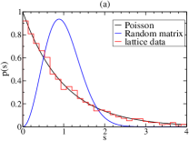
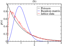
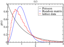
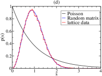
Figure 1: The unfolded level spacing distribution in different regions of the Dirac spectrum. The panels from (a) through (d) correspond to spectral windows going up in the spectrum. The dashed line indicates the exponential distribution corresponding to the localized (Poisson) case and the dotted line indicates the chiral unitary Wigner surmise expected in the delocalized (RMT) case.

Unfolding eliminates non-universal features of the spectral statistics and the resulting ULSD is fully universal. For localized eigenmodes and Poisson statistics the ULSD is the standard exponential distribution,

$$P(s)=\exp(-s).$$ (3)

For delocalized modes the ULSD can still be computed analytically and it is very precisely approximated by the Wigner surmise of the corresponding random matrix universality class. QCD with staggered quarks in the fundamental representation belongs to the unitary class and the corresponding Wigner surmise is

$$P(s)=\dfrac{32}{\pi^{2}}s^{2}\cdot\exp\left(-\dfrac{4}{\pi}s^{2}\right).$$ (4)

It is remarkable that these distributions do not have any free parameters and thus a precise agreement of the ULSD with either of these is a strong indication for the corresponding eigenmodes to be localized or delocalized respectively.

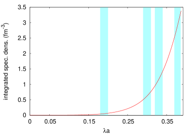
Figure 2: The integrated spectral density, normalized by the volume, in units of fm^-3 in the spectrum across the transition. The mobility edge is at $\lambda_{c}a=0.336$. The boxes correspond to the spectral windows of Fig. 1.

To demonstrate the transition from localized to delocalized states within the QCD Dirac spectrum, in Fig. 1 we show the ULSD in four different spectral windows starting from the lowest part of the spectrum and going upwards. The data is based on simulations with $N_{f}=2+1$ flavors of stout smeared staggered quarks. The temporal lattice size was $N_{t}=4$ and the lattice spacing $a=0.125$ fm, which corresponds to a temperature of $T=400$ MeV. Details of the action and the scale setting can be found in Ref. Aoki:2005vt . We also show the predictions for the ULSD coming from Poisson statistics and from RMT in Eqs. (3) and (4) respectively. It is clear that starting from the lowest modes and going upwards, the spectrum undergoes a transition from Poisson to Wigner-Dyson statistics. It is interesting to compare this with how the spectral density increases throughout the spectrum. In Fig. 2 we plot the integrated spectral density in the spectrum through the transition.

V Finite size scaling and the correlation length critical exponent

The transition in the spectral statistics is a clear indication that a localization-delocalization type transition takes place in the QCD Dirac spectrum. On the other hand, there is a finite spectral window where the statistics is clearly in between the two universal possibilities already indicated. This is, however, not unexpected. Transitions in finite systems are always smooth, and genuine critical behavior, exhibiting sharp transitions, can only occur in the thermodynamic limit. One possibility to decide whether there is such a transition for an infinite system is to study the dependence of the transition on the system size using finite size scaling. In this section we summarize the results of a finite size scaling study of the transition in the QCD spectrum. For more technical details of this analysis we refer the reader to Ref. Giordano:2013taa .

To quantify the sharpness of the transition we choose a particular quantity characterizing the unfolded level spacing distribution and monitor how it changes through the transition in systems of various sizes. In principle, any quantity that has different values for the limiting distributions of Eqs. (3) and (4) would be suitable for this purpose. A convenient choice is the integral of the probability density

$$I=\int_{0}^{s_{0}}P(s)\,ds$$ (5)

to the point $s_{0}\approx 0.5$ where the two limiting distributions cross. For our purposes $I$ is a good quantity since it decreases monotonically from the exponential to the Wigner-Dyson distribution and the difference of the values it takes in the limiting cases is large enough. At the same time $I$ receives contributions from a substantial fraction of the modes following the exponential distribution. This helps to improve the quality of the observable at the low-end of the spectrum where the statistics is otherwise rather limited due to the small spectral density there.

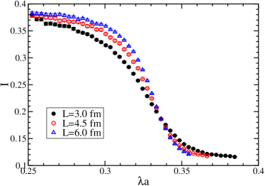
Figure 3: The quantity $I$ defined by Eq. (5) computed in narrow spectral windows across the transition. The different symbols represent data taken from systems of different spatial sizes indicated in the legends.

In Fig. 3 we show this quantity computed separately in different spectral windows across the spectrum. The different symbols correspond to linear spatial sizes of $L=3.0,4.5$ and $6.0$ fm. The transition clearly becomes sharper as the spatial volume of the system increases.

To obtain a more quantitative description of the dependence of the transition on the linear size of the system, $L$, we use finite size scaling based on a renormalization group (RG) argument. As is usual in Anderson transitions, we assume a single relevant variable controlling the correlation length. In our setup this can be taken to be $\lambda$, the location in the spectrum. To simplify the notation, in the following discussion we write $\lambda$ instead of $\lambda-\lambda_{c}$ where $\lambda_{c}$ is the mobility edge, that is the critical point in the spectrum where the transition occurs. We have to keep in mind that $\lambda_{c}$ is a parameter that also has to be determined from the finite size scaling.

We assume that the quantity $I$ that we consider here depends on $\lambda$, $L$ and some leading irrelevant variable that we call $\mu$. A blocking transformation with scale $b>1$ transforms these parameters as

$$\lambda\rightarrow b^{1/\nu}\lambda,\hskip 8.61108ptL\rightarrow b^{-1}L,\hskip 8.61108pt\mu\rightarrow b^{y_{\mu}}\mu,$$ (6)

where $\nu>0$ is the correlation length critical exponent and $y_{\mu}<0$ is the leading (smallest magnitude) irrelevant exponent and we used the linear approximation of the blocking transformation around the given fixed point. Other irrelevant operators are neglected. Since $I$ is a dimensionless RG-invariant quantity it does not change under a scale $b$ blocking transformation. It means that

$$I(\lambda,\mu,L)\;=\;I(b^{1/\nu}\lambda,b^{y_{\mu}}\mu,b^{-1}L).$$ (7)

Choosing the blocking factor $b$ to be proportional to the system size, $b=L/C$, systems of various sizes can be blocked down to the same “reference size” $C$ and compared. In this way the dependence of $I$ on the system size through its last argument can be eliminated and

$$I(\lambda,\mu,L) =\;I((CL)^{1/\nu}\lambda,(CL)^{y_{\mu}}\mu,C)\;$$ (8)

$$=\;f(L^{1/\nu}\lambda,L^{y_{\mu}}\mu),$$

where $f$ is a scaling function. Since $y_{\mu}$, being the exponent of an irrelevant operator, is negative, in principle the size of the system can be chosen large enough for $L^{y_{\mu}}\mu\approx 0$ and then $I$ depends only on the single variable $L^{1/\nu}\lambda$. Note that since the correlation length in an infinite system is proportional to $\lambda^{-\nu}$, this single independent variable is essentially the ratio of the system size and the correlation length.

Singular behavior is not expected in a finite system and as a result the dependence of $I$ on $\lambda$ is analytic and can be expanded as

$$I(\lambda,L)=F(L^{1/\nu}(\lambda-\lambda_{c}))=\sum_{n}F_{n}L^{\frac{n}{\nu}}(\lambda-\lambda_{c})^{n},$$ (9)

where we have restored the explicit dependence on the critical point, $\lambda_{c}$.

Finite size scaling relies on the first equality of Eq. (9). This means that data for $I$ computed on systems of different sizes, if plotted as a function of the appropriate scaling variable $L^{1/\nu}(\lambda-\lambda_{c})$, should all collapse on a single scaling curve . Our task is to determine the parameters $\lambda_{c}$ and $\nu$ resulting in such data collapse (see Fig. 4). The simplest way of doing that is by making use of the expansion in Eq. (9), truncated to an appropriate order, $n$. Data taken on different volumes can be fitted to this form to extract the parameters $\lambda_{c},\nu$ and $F_{0},F_{1},\ldots,F_{n}$. The truncation order, $n$, should be large enough to properly describe the scaling function, $F$, in the fitting range but small enough to ensure stability of the fits.

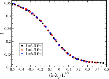
Figure 4: The quantity $I$ defined by Eq. (5) computed in narrow spectral windows across the transition. The different symbols represent data taken from systems of different spatial sizes indicated in the legends. The data is plotted against the scaling variable $L^{1/\nu}(\lambda-\lambda_{c})$ with the parameters $\nu$ and $\lambda_{c}$ obtained from the fit (see text).

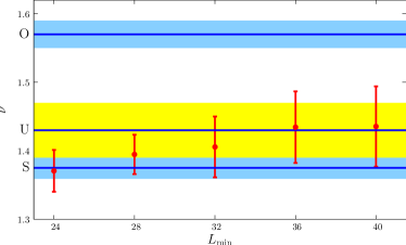
Figure 5: (Reprinted from Ref. Giordano:2013taa ) The fitted value of the critical exponent $\nu$ versus $L_{\mbox{\scriptsize min}}$, the linear size of the smallest system for which data was included in the fit. The three horizontal lines and shaded regions represent the critical exponents and their uncertainties for the Anderson models of orthogonal, unitary and symplectic symmetry classes (marked from top to bottom and obtained from Refs. corrections ; nu_unitary ; nu_symp ).

This procedure gives correct results only if the volumes included in the fit are large enough that corrections coming from the neglected irrelevant parameter(s) (see Eq. (8)) are small. Such corrections can be systematically accounted for by replacing Eq. (9) with a double expansion containing also the dependence of $I$ on the leading irrelevant variable, $\mu$. However, this makes the number of parameters to be fitted so large that very good quality data is needed to ensure a stable fit. For this reason we followed a different procedure. We did the fit using only subsets of the full data by omitting data for system sizes smaller than $L_{\mbox{\scriptsize min}}$. In Fig. 5 we show how the fitted value of the exponent $\nu$ depends on the smallest system size that is included in the fit. Naturally, if less data is used for the fit, its uncertainty increases but the fitted value stabilizes, showing that corrections to the assumed one-parameter scaling of Eq. (9) are not larger than the other sources of uncertainty. It is remarkable that the critical exponent we obtain for the QCD transition is consistent with that of the unitary Anderson model. This strongly indicates the these two seemingly very different models are in the same universality class.

VI Continuum limit and the temperature dependence of the mobility edge

We have demonstrated that the transition in the QCD Dirac spectrum is a genuine Anderson transition belonging to the same universality class as the Anderson model of the corresponding (unitary) symmetry class. However, this was done only at a fixed lattice spacing. Since the physical theory is defined only as the continuum limit of lattice QCD, it is important to check how the transition changes in the continuum limit. In this respect the most important quantity to look at is the mobility edge, $\lambda_{c}$. In finite temperature lattice simulations the temperature is controlled by the system size in the temporal direction as

$$T=\frac{1}{N_{t}a},$$ (10)

where $N_{t}$ is the temporal size of the box in lattice units and $a$ is the lattice spacing. Since $N_{t}$ is typically a small integer, if the lattice spacing is fixed, the temperature can be changed only in discrete steps. For this reason, in Ref. Kovacs:2012zq we studied both the temperature and the lattice spacing dependence of the mobility edge using the same set of simulations. For this we combined three different lattice spacings, $a=0.125,0.082$ and $0.062$ fm with $N_{t}=4,6,8$ (not all combinations were used). The parameters were chosen so that at $T=400$ MeV we had simulations with all three lattice spacings and the temperatures spanned the range between 260 MeV and 800 MeV.

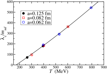
Figure 6: (Reprinted from Ref. Kovacs:2012zq ) The mobility edge normalized by the light quark mass versus the temperature. Different symbols represent data originating from simulations with different lattice spacings. The continuous line is a quadratic fit to all the data.

The mobility edge is a dimensionful quantity and it is not a renormalization group invariant. Since $\lambda_{c}$ characterizes the Dirac spectrum, it is expected to be renormalized as the quark mass (see Refs. Giusti:2008vb and Kovacs:2012zq for a discussion). For this reason the quantity that we considered was $\lambda_{c}/m_{\mbox{\scriptsize ud}}$, the mobility edge normalized by the light quark mass. In Fig. 6 we show the temperature dependence of this quantity. Since the data obtained at different lattice spacings are all on a smooth curve, we can conclude that scaling violations are small and the Anderson transition also takes place in the continuum limit.

Also in the same figure we show a quadratic fit of the form

$$\frac{\lambda_{c}}{m_{\mbox{\scriptsize ud}}}(T)=a\cdot\frac{T-T_{c}}{T_{c}}+b\cdot\left(\frac{T-T_{c}}{T_{c}}\right)^{2}$$ (11)

By construction, $T_{c}$ is the temperature where the mobility edge vanishes and, as a result, the Anderson transition ceases to exist. The fit yields $T_{c}=171(9)$ MeV which is consistent with the known location of the cross-over Borsanyi:2010bp ; Bazavov:2011nk . We also note that in Eq. (11) the dimensionless coefficient of the quadratic term coming from the fit is two orders of magnitude smaller than that of the linear term. The mobility edge thus increases sharply with the temperature and, to a good approximation, it scales linearly with the temperature.

VII Shape analysis

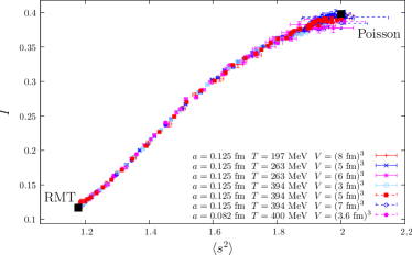
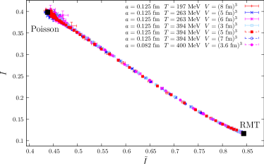
Figure 7: Shape analysis using $I$ (Eq. (5)) and the second moment of the ULSD $\langle s^{2}\rangle$ (top), and $I$ and $\tilde{I}$ (Eq. (12)) (bottom).

In Section V we analyzed in detail how $I$ changed in the spectrum through the Anderson transition. Our finite size scaling analysis was essentially based on a matching of points in the spectra of systems of different sizes where $I$ took the same value. That such a matching was possible by a simple transformation $\lambda\rightarrow L^{1/\nu}(\lambda-\lambda_{c})$ was indirect evidence that $I$ depended only on the ratio of the system size to the correlation length. This is natural to expect in the case of an Anderson transition since there is only one relevant variable around the fixed point characterizing the transition.

The quantity $I$ is just one parameter characterizing the ULSD. Through the transition the ULSD changes from the exponential distribution to the Wigner surmise in a continuous way. Thus the ULSD traverses a path in the infinite dimensional space of all possible distributions. An interesting question is how this path depends on the particular details of the system such as the volume, the lattice spacing and the physical temperature. A simple way to study this, known as shape analysis shape_analysis , is to compute different parameters of the ULSD and plot them one against another. If the ULSD of different systems follows the same universal path, the data coming from these systems should collapse on a single universal curve. This curve can be viewed as a two dimensional projection of the path that the ULSD traces.

In Fig. 7 we show the results of the shape analysis for two pairs of observables, namely $I$ and the second moment of the ULSD, and $I$ and the integrated ULSD $\tilde{I}$, defined as

$$\tilde{I}=\int_{s_{0}}^{s_{1}}ds\,P_{\lambda}(s)\,,$$ (12)

where $s_{1}\approx 1.8$ is the second crossing point of the exponential and the Wigner surmise. Data obtained with different lattice size, lattice spacing and/or temperature all fall on a universal curve, with deviations being smaller than the statistical errors for both pairs of observables. From this analysis one can conclude that the transition from Poisson to Wigner-Dyson statistics takes place on a universal path, up to small corrections. In turn, this hints to the local spectral statistics depending on the position in the spectrum and on the details of the system through a single quantity $\zeta$, i.e., the local ULSD $P=P(s;\lambda;L,a,T)$ is a function of the form $P(s;\lambda;L,a,T)=p(s;\zeta(\lambda,L,a,T))$, up to small corrections vanishing in the limit $L\to\infty$. In other words, the local ULSD is essentially determined by a single physical quantity, which is most likely a property of the corresponding eigenvectors, regardless of the details of the system. A natural candidate is the correlation length of the eigenvectors, which certainly is the appropriate quantity in the vicinity of the critical point, where one-parameter scaling applies.

The universal path in the space of probability distributions corresponds to a universal one-parameter family of random matrix models, describing the transition from Poisson to Wigner-Dyson behavior in the Dirac spectrum independently of the details of the system. A comparison with analogous results obtained in the Anderson model shows that the spectral statistics at the critical point in the two models are compatible Nishigaki . This provides further support to the claim that the localization/delocalization transitions found in the two models belong to the same universality class.

VIII Conclusions

We studied the transition from localized to delocalized states in the QCD Dirac spectrum at high temperature. We demonstrated that the transition is a genuine Anderson transition and that its critical exponent agrees with that of the corresponding Anderson model. However, there is an important difference between Anderson transitions in electronic systems and the transition in QCD. On the one hand, in electronic systems the Anderson transition is a genuine phase transition with the zero temperature conductivity having a singularity. On the other hand, in QCD, most likely there is no singular thermodynamic behavior associated with the Anderson transition. In fact, the finite temperature transition from the hadronic to the quark-gluon plasma state is known to be a cross-over Aoki:2006we . The resolution of this apparent paradox is that the QCD Dirac spectrum has no such direct physical interpretation as the spectrum of the one-electron Hamiltonian. Neither the appearance of low-lying localized states around $T_{c}$ nor the presence of a mobility edge above $T_{c}$ manifests itself in singular thermodynamic behavior. This is because there is no thermodynamic quantity in QCD that is sensitive enough to the abrupt change occurring at $\lambda_{c}$ in the spectrum.

However, this might not be the case for some other QCD-like theories. It is believed that if the quark masses were small enough the finite temperature cross-over would become a phase transition pisarski-wilczek . In that case the extension of the singular line $\lambda_{c}(T)$ in the “phase diagram” of Fig. 6 to $T_{c}$ might contain useful information about the chiral phase transition.

Even though in QCD the Anderson transition does not correspond to a genuine phase transition in observable quantities, the appearance of localized states in the Dirac spectrum can have important physical consequences. Correlators of hadronic operators can be written in terms of quark propagators which in turn admit a decomposition into Dirac eigenmodes. The eigenmodes in this decomposition are weighted with $(m+i\lambda)^{-1}$ where $m$ is the quark mass and $\lambda$ is the eigenvalue. Low-lying Dirac modes, therefore, give a large contribution to correlators. However, they can give a significant contribution to the correlators only on distance scales smaller than their localization length. Therefore, long-distance correlators are dominated by Dirac eigenmodes above the mobility edge. In this way the mobility edge plays the role of an effective gap in the spectrum, similar to the quark mass. In this connection it is remarkable that this gap increases sharply with the temperature and even around $T=2T_{c}$ it is already two orders of magnitude larger than the light quark mass (see Fig. 6). Asymptotic hadronic correlators at and above this temperature behave qualitatively as if the effective quark mass were comparable to $\lambda_{c}$. This might provide an explanation of the sharp increase of screening masses that was observed in lattice calculations above $T_{c}$ Cheng:2010fe .

There are several directions in which further study can provide interesting new insight. Firstly, the full physical implications of localized Dirac modes have certainly not been understood. The possible connections, if any, of the QCD Anderson transition to finite temperature phase transitions in QCD-like theories still remains to be explored. Secondly, there is much more to be learned from a detailed study of how the quark eigenmodes themselves change through the transition. The only information we have about this so far is through the inverse participation ratio (IPR). Using the IPR we estimated that the localization length of the localized modes is controlled by the inverse temperature Kovacs:2012zq . In Anderson transitions, however, it is known that the critical wave functions develop a peculiar multifractal structure that has recently been utilized to improve the finite size scaling analysis multifractal . It would be certainly interesting to explore this possibility in the QCD Anderson transition.

Both the Anderson model and the lattice QCD Dirac operator are sparse random matrices with a structure reflecting the geometry of space (or space-time). In this context it would be interesting to understand what are the necessary conditions of an Anderson-type transition in the spectrum of such a system. One might be tempted to speculate that it is the spectral density per unit volume that drives the transition. Indeed, a small spectral density per unit volume is almost surely a necessary condition for localized modes to appear, as otherwise fluctuations of the gauge field are likely to mix the modes due to their small energy differences. However, that this is certainly not the full story is shown by the example of QCD-like theories with many fermion flavors. Introducing enough fermion flavors can drive those systems into the deconfined chirally restored phase already at zero temperature; as a result, the spectral density at the low-end of the spectrum becomes arbitrarily small. However, no Anderson transition takes place in those systems Landa-Marban:2013oia ; Bietenholz:2013coa . This example also shows that there is much to be understood about Anderson transitions in QCD-like theories.

Finally, we would like to remark that phenomena apparently similar to the one described here were previously seen in quenched QCD at zero temperature. Golterman and Shamir found that just outside the Aoki phase there is a finite density of localized Dirac modes related to so called exceptional configurations, topological charge fluctuations on the scale of the lattice spacing Golterman:2003qe . However, these objects are very different from the ones that we studied here, as they are not driven by the temperature and are expected to be absent in the full theory with light dynamical quarks. Greensite et al. observed that in zero temperature quenched gauge backgrounds the covariant Laplacian also possesses localized eigenmodes at the edge of its spectrum Greensite:2005yu . Also in this case there is no indication that this phenomenon could be related to the transition in the spectrum at finite temperature described in the present paper.

References

- (1) T. G. Kovács and F. Pittler, Phys. Rev. Lett. 105, 192001 (2010) [arXiv:1006.1205 [hep-lat]].
- (2) P. W. Anderson, Phys. Rev. 109, 1492 (1958).
- (3) R. Dalichaouch, J.P. Armstrong, S. Schultz, P.M. Platzman, and S. L. McCall, Nature 354, 53 (1991).
- (4) H. Hu, A. Strybulevych, J.H. Page, S.E. Skipetrov, and B.A. Van Tiggelen, Nature Physics 4, 945 (2008).
- (5) J. Billy et al., Nature 453, 891 (2008); G. Roati et al., Nature 453, 895 (2008).
- (6) J. J. M. Verbaarschot and T. Wettig, Ann. Rev. Nucl. Part. Sci. 50, 343 (2000) [arXiv:hep-ph/0003017].
- (7) T. G. Kovács and F. Pittler, Phys. Rev. D 86, 114515 (2012) [arXiv:1208.3475 [hep-lat]].
- (8) M. Giordano, T. G. Kovács and F. Pittler, Phys. Rev. Lett. 112, 102002 (2014) [arXiv:1312.1179 [hep-lat]].
- (9) L. Susskind, Phys. Rev. D 16, 3031 (1977).
- (10) J. B. Kogut and L. Susskind, Phys. Rev. D 11, 395 (1975).
- (11) T. Banks et al. [Cornell-Oxford-Tel Aviv-Yeshiva Collaboration], Phys. Rev. D 15, 1111 (1977).
- (12) I. Montvay and G. Münster, “Quantum fields on a lattice,” Cambridge, UK: Univ. Pr. (1994) 491 p. (Cambridge monographs on mathematical physics).
- (13) A. M. Halász and J. J. M. Verbaarschot, Phys. Rev. Lett. 74, 3920 (1995) [hep-lat/9501025].
- (14) A. M. García-García and J. C. Osborn, Phys. Rev. D 75, 034503 (2007) [arXiv:hep-lat/0611019].
- (15) R. Narayanan and H. Neuberger, Phys. Rev. Lett. 71 (1993) 3251 [arXiv:hep-lat/9308011].
- (16) R. Narayanan and H. Neuberger, Nucl. Phys. B 412, 574 (1994) [arXiv:hep-lat/9307006].
- (17) R. Narayanan and H. Neuberger, Nucl. Phys. B 443, 305 (1995) [arXiv:hep-th/9411108].
- (18) H. Neuberger, Phys. Lett. B 417, 141 (1998) [hep-lat/9707022].
- (19) T. G. Kovács, Phys. Rev. Lett. 104, 031601 (2010) [arXiv:0906.5373 [hep-lat]].
- (20) T. Guhr, A. Müller-Groeling and H. A. Weidenmuller, Phys. Rept. 299, 189 (1998) [cond-mat/9707301].
- (21) Y. Aoki, Z. Fodor, S. D. Katz and K. K. Szabó, JHEP 0601, 089 (2006) [hep-lat/0510084];
- (22) K. Slevin and T. Ohtsuki, Phys. Rev. Lett. 82, 382 (1999).
- (23) K. Slevin and T. Ohtsuki, Phys. Rev. Lett. 78, 4083 (1997).
- (24) Y. Asada, K. Slevin and T. Ohtsuki, J. Phys. Soc. Jpn. 74 supplement, 238 (2005) [cond-mat/0410190 [cond-mat.dis-nn]].
- (25) L. Giusti and M. Lüscher, JHEP 0903, 013 (2009) [arXiv:0812.3638 [hep-lat]].
- (26) S. Borsányi et al. [Wuppertal-Budapest Collaboration], JHEP 1009, 073 (2010) [arXiv:1005.3508 [hep-lat]];
- (27) A. Bazavov, T. Bhattacharya, M. Cheng, C. DeTar, H. T. Ding, S. Gottlieb, R. Gupta and P. Hegde et al., Phys. Rev. D 85, 054503 (2012) [arXiv:1111.1710 [hep-lat]].
- (28) I. Varga, E. Hofstetter, M. Schreiber and J. Pipek, Phys. Rev. B 52, 7783 (1995).
- (29) S.M. Nishigaki, M. Giordano, T.G. Kovács and F. Pittler, PoS LATTICE 2013, 018 (2013).
- (30) Y. Aoki, G. Endrődi, Z. Fodor, S. D. Katz and K. K. Szabó, Nature 443, 675 (2006) [hep-lat/0611014].
- (31) R. D. Pisarski and F. Wilczek, Phys. Rev. D 29, 338 (1984).
- (32) M. Cheng, S. Datta, A. Francis, J. van der Heide, C. Jung, O. Kaczmarek, F. Karsch and E. Laermann et al., Eur. Phys. J. C 71, 1564 (2011) [arXiv:1010.1216 [hep-lat]].
- (33) A. Rodriguez, L.J. Vasquez, K. Slevin and R.A. Römer, Phys. Rev. Lett. 105, 046403 (2010); Phys. Rev. B 84, 134209 (2011).
- (34) D. Landa-Marbán, W. Bietenholz and I. Hip, arXiv:1307.0231 [hep-lat];
- (35) W. Bietenholz, I. Hip and D. Landa-Marbán, arXiv:1310.3427 [hep-lat].
- (36) M. Golterman and Y. Shamir, Phys. Rev. D 68, 074501 (2003) [hep-lat/0306002].
- (37) J. Greensite, S. Olejník, M. Polikarpov, S. Syritsyn and V. Zakharov, Phys. Rev. D 71, 114507 (2005) [hep-lat/0504008].