An in situ measurement of the radio-frequency attenuation in ice at Summit Station, Greenland

Abstract

We report an in situ measurement of the electric field attenuation length $L_{\alpha}$ at radio frequencies for the bulk ice at Summit Station, Greenland, made by broadcasting radio-frequency signals vertically through the ice and measuring the relative power in the return ground bounce signal. We find the depth-averaged field attenuation length to be $\langle L_{\alpha}\rangle=947^{+92}_{-85}$ m at 75 MHz. While this measurement has clear radioglaciological applications, the radio clarity of the ice also has implications for the detection of ultra-high energy (UHE) astrophysical particles via their radio emission in dielectric media such as ice. Assuming a reliable extrapolation to higher frequencies, the measured attenuation length at Summit Station is comparable to previously measured radio-frequency attenuation lengths at candidate particle detector sites around the world, and strengthens the case for Summit Station as a promising northern site for UHE neutrino detection.

1 Introduction

We report a measurement of the radio-frequency electric field attenuation length in the ice at the Summit Station site in Greenland. Our interest in the radio properties of glacial ice stems from the applications to particle astrophysics, but these measurements are also of interest for the development of radar systems that probe sub-surface features in glacial ice, such as ice strata and sub-glacial lakes and streams.

We are ultimately interested in building a detector to search for radio emission created when the highest energy astrophysical neutrinos interact in a large volume of a dielectric material (?????). Glaciers are the leading candidate medium for a detector for ultra-high energy (UHE) neutrinos because the cold ice temperature leads to a long radio attenuation length (?) and they have large volume. These two properties combine to allow for a large enough instrumented detector volume to have the sensitivity required to detect significant numbers of UHE neutrinos, which are very rare (?).

When a neutrino interacts with a dielectric material, such as glacial ice, it initiates a shower of charged particles approximately 0.1 m in diameter and tens of meters long. The charged particles in the shower move faster than the speed of light in the medium, which is reduced compared to the speed of light in a vacuum by the index of refraction of ice, $n$. This causes Cerenkov radiation, the electromagnetic analogue to a sonic boom. Because the size of the particle shower is small compared to the wavelength of radio waves, the radio component is emitted coherently at frequencies up to a few GHz, and for high-energy showers is the strongest component of the radiation (?). This coherence effect was later confirmed in the laboratory in a variety of media, including ice, using showers initiated by high-energy electron and photon beams (??).

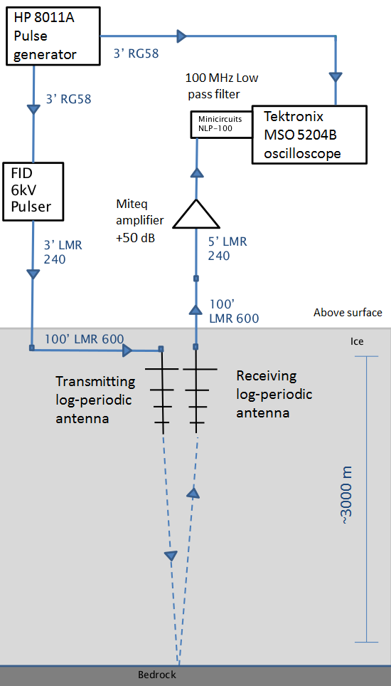
Figure 1: A drawing of the experimental setup for the ground bounce with low-frequency antennas. We used a FID Technologies 6 kV high voltage pulser, triggered by a Hewlett Packard 8011A pulse generator to transmit through a log-periodic antenna. We used a second log-periodic antenna coupled to a $+50$ dB Miteq amplifier to boost the received signal and a Tektronix MSO5204B to record the data.

The distance the radio-frequency signals can propagate depends on the properties of the glacial ice at the specific site; the attenuation length varies from site to site by large factors. Attenuation length corresponds to the rate of neutrino detection, so in situ measurements at specific sites are essential. Previous measurements have been made of the radio properties of the ice at sites in Antarctica (Taylor Dome, the South Pole, and the Ross Ice Shelf) to determine the best southern sites for UHE neutrino detection (?????), and have found a depth-averaged field attenuation length $\langle L_{\alpha}\rangle$ at 300 MHz of $1660^{+255}_{-120}$ m over the top 1500 m of ice at the South Pole (?).

There have been previous measurements in the frequency range of interest (hundreds of MHz) at Summit Station that have investigated layering in the ice (?) for their glaciologic implications, and the radar attenuation length has recently been measured at many sites across the Greenland Ice Sheet (?). In this paper, we report an in situ measurement of the radio attenuation length of the bulk glacial ice at the Summit Station site made using similar methods to previous measurements at other sites (?????).

2 Experimental Approach

Our approach is similar to previous work in our field (???). From the surface, we transmit a high-voltage impulse with broadband frequency content into the ice and measure the power in the return signal as a function of frequency with a second, identical antenna. We compare this ground bounce to the transmission of the same impulse through a short distance in air, directly from one antenna to the other. After accounting for the geometric factor $1/r$ (for electric field strength), where $r$ is the propagation distance, the remaining loss in electric field in the ground bounce return pulse is attributed to attenuation and scattering in the ice, which goes as $\mathrm{exp}(-r/\langle L_{\alpha}\rangle)$. We use this technique of comparing the through-air data to the in-ice data, rather than calculating the expected power in the return ground bounce signal from the known power transmitted by the system, to reduce systematic uncertainty.

We adopt a similar notation and technique to ?. We define $P_{\nu}$ to be the power spectral density at frequency $\nu$ of the impulse as received by a $50~{}\Omega$ receiver, and $V_{\nu}$ to be $\sqrt{P_{\nu}\times 50~{}\Omega}$. The quantity $V_{\nu,\mathrm{ice}}$ is $V_{\nu}$ measured after passing through the ice, bouncing off of the bedrock, and traveling back to the receiver over a total distance $d_{\mathrm{ice}}$, and $V_{\nu,\mathrm{air}}$ is $V_{\nu}$ after being transmitted directly through the air between the two antennas separated by $d_{\mathrm{air}}$.

Therefore,

$$V_{\nu,\mathrm{ice}}/V_{\nu,\mathrm{air}}=(d_{\mathrm{air}}/d_{\mathrm{ice}})e^{-d_{\mathrm{ice}}/\langle L_{\alpha}\rangle},$$ (1)

where $\langle L_{\alpha}\rangle$ is the depth-averaged field attenuation length over the entire depth of the ice.

Solving for $\langle L_{\alpha}\rangle$ gives

$$\langle L_{\alpha}\rangle=d_{\mathrm{ice}}/\ln(\frac{V_{\nu,\mathrm{air}}~{}d_{\mathrm{air}}}{V_{\nu,\mathrm{ice}}~{}d_{\mathrm{ice}}}).$$ (2)

The ratio of the power transmitted by the antenna into ice compared to air, $T_{\mathrm{ratio}}$, due to a small difference in coupling between the antenna and ice compared to air, affects the measured attenuation length $\langle L_{\alpha}\rangle$. The assumed power reflection coefficient $R$ at the ice-bedrock interface also affects the measured $\langle L_{\alpha}\rangle$. Including both of these effects, $\langle L_{\alpha}\rangle$ becomes

$$\langle L_{\alpha}\rangle=d_{\mathrm{ice}}/\ln(T_{\mathrm{ratio}}~{}\sqrt{R}~{}\frac{V_{\nu,\mathrm{air}}~{}d_{\mathrm{air}}}{V_{\nu,\mathrm{ice}}~{}d_{\mathrm{ice}}}).$$ (3)

In the above equation, we have included a factor of $\sqrt{T_{\mathrm{ratio}}}$ for the relative transmission of electric field for each antenna (the transmitter and the receiver), yielding a total factor of $T_{\mathrm{ratio}}$.

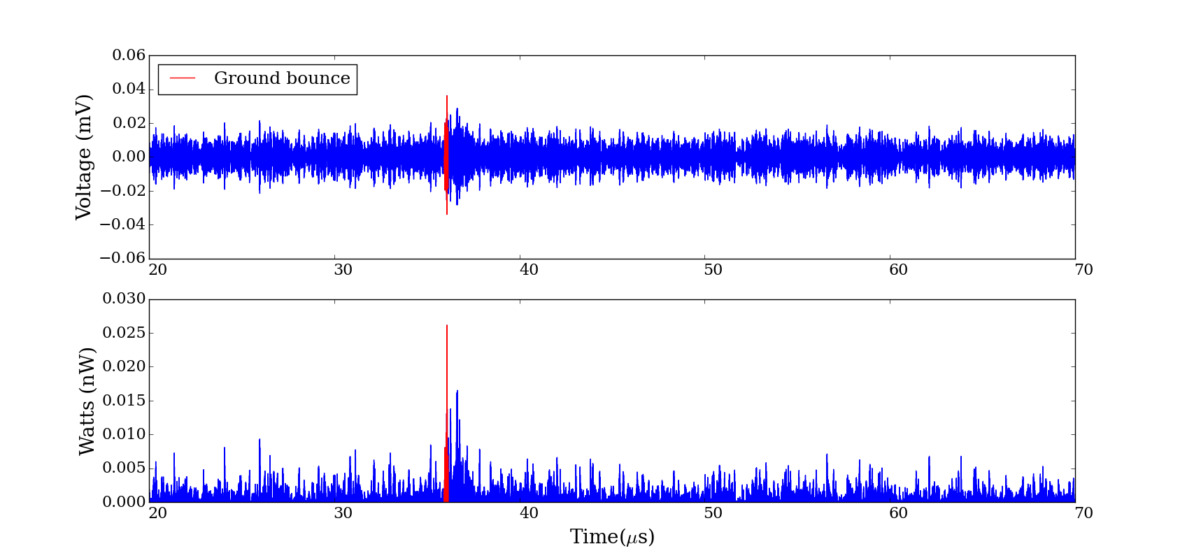
Figure 2: Top: The received voltage in a 50 $\Omega$ receiver as a function of time with the log-periodic antennas buried in the snow, pointed downward. A large reflection is evident at 36.1 $\mu$s (highlighted in red), consistent with a depth of $3014^{+48}_{-50}$ m. Bottom: The power received as a function of time, derived from the top panel. The red region denotes the 200 ns wide time window used for analysis.

2.1 Experimental Setup

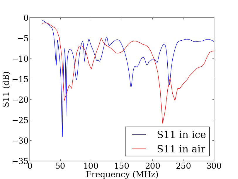
Figure 3: The return loss ($\mathrm{S}_{11}$) of the log-periodic antenna used for the ground bounce measurement for the antenna buried below the surface and packed with snow (blue), compared to the same antenna in air (red).

The measurement that we report here was performed in June 2013 at the Summit Station site, and is a ground bounce, described above and shown in a sketch in Figure 1. The measurements were made at N 72^∘ 37’ 20.7” W 38^∘ 27’ 34.7”, near Summit Station, the highest point on the Greenland ice sheet. We transmitted a fast, high-voltage impulsive signal, generated by a FID Technologies 6 kV high-voltage pulser. The high-voltage pulser was triggered by a Hewlett Packard 8011A pulse generator, which also triggered the oscilloscope that recorded the received signal. We transmitted the high-voltage impulse through 30 m of LMR-600 cable before sending it out of a high gain antenna aimed down toward the bottom of the glacier. We received the signal with an identical antenna, also aimed downward, 46 m away along the surface of the snow. We then amplified the received signal with a Miteq amplifier ($+50$ dB of gain, model AFS3-00200120-10-1P-4-L) before passing it through a 100 MHz low-pass filter and reading it out with a Tektronix MSO5204B oscilloscope that was set to average over 10,000 impulses. We included the 100 MHz low-pass filter in the system to reduce intermittent noise pickup from man-made sources. The antennas were buried in the snow and packed with snow to ensure the best coupling between the antenna and the snow, reducing Fresnel effects at the snow-air interface.

To record the signal that we transmitted through the system, we also took data with the antennas aimed toward each other through the air, 46 m apart. This normalization run through air had the same cabling and setup as the ground bounce measurement, but with an additional 40 dB attenuator on the input to the Miteq amplifier to avoid saturating the amplifier with the large signal.

To reduce the effect of reflections off of the surface of the snow in the normalization run through air, we took data with the antennas 2 m above the surface of the snow. We tested that the effect of reflections off of the surface of the ice on the received signal is small by varying the height of the antennas and looking for changes in the observed signal and saw none. We also used these antennas previously for testing in a high bay in a similar configuration, and placed radio frequency absorber along the surface of the floor and observed no significant change to the signal.

We used a pair of log-periodic antennas with good transmission between 60 and 100 MHz and $\sim 6$ dBi of gain. The return loss ($\mathrm{S}_{11}$) of the log-periodic antenna when buried below the surface and packed with snow compared to the antenna in air is shown in Figure 3. The transmission band of the antenna moves down slightly in frequency when coupled to the snow, evidenced by the change in the -3 dB point of the antenna and expected from the higher index of refraction of snow compared to air. There is good transmission in the frequency range used in analysis (65-85 MHz) in air and when coupled to the firn.

2.2 Data Analysis

The top panel of Figure 2 shows a long trace recorded with the low-frequency antennas pointed downward and buried in the snow. The bottom panel of the figure is the power in the return signal as a function of time, derived from the top panel. The trace has been filtered to 65-85 MHz using a Butterworth filter of order three to limit the noise contribution out of the band of the system (defined at the low frequency end by the antenna transmission coefficient and the high frequency end by the low-pass filter) and extract a clear signal. There is a clear reflection at an absolute time of 36.1 $\mu$s, which is consistent with the timing expected for a signal that bounced off of the ice-bedrock interface at a depth known from GRIP borehole measurements (?). From the absolute time of 36.1 $\mu$s, accounting for the measured system delay of 430 ns, we can measure the total round-trip distance through the ice, $d_{\mathrm{ice}}$, using the relationship

$$d_{ice}=c_{n}\Delta t,$$ (4)

where $c_{n}$ is the speed of light in the medium and $\Delta t$ is the total time of flight through the ice. $c_{n}$ is related to the dielectric constant of the medium via

$$c_{n}=\frac{c}{\sqrt{\epsilon^{\prime}}},$$ (5)

where $c$ is the speed of light in a vacuum and $\epsilon^{\prime}$ is the real component of the complex dielectric constant of the material. The index of refraction of the medium, $n$, is equal to $\sqrt{\epsilon^{\prime}}$. We use a firn model based on the measured density profile, $\rho$, at Summit Station from ? to determine the index of refraction as a function of depth for the firn layer. Our firn model has two regimes: one that describes the density from the surface to $15$ m below the surface, and a second that describes the firn from $15$ m to $100$ m below the surface. By $100$ m, the firn has transitioned to glacial ice. For radio propagation in glacial ice, the dielectric constant is related to the density of the ice (?) by

$$\epsilon^{\prime}=(1+0.845\rho)^{2},$$ (6)

allowing us to calculate $n$, and subsequently $c_{n}$, as a function of depth for the firn. We assume an index of refraction of glacial bulk ice of $1.78\pm 0.03$ for ice below $100$ m deep (?). We calculate that the depth of the observed ground bounce is $3014^{+48}_{-50}$ m, which leads to $d_{\mathrm{ice}}=6028^{+96}_{-100}$ m. This is consistent with the known depth of the ice at Summit Station from GRIP borehole measurements (?).

We note that there is a second and smaller reflection $0.6$ $\mu$s after this initial ground bounce (corresponding to 91 m farther). In principle, it is valid to choose any return signal, as long as we include the correct distance to the bounce in our calculations and make a realistic assumption about the power reflection coefficient at the interface, $R$. In practice, we ran our data analysis over each of the two return impulses (36.1 $\mu$s and 36.7 $\mu$s), and there is little difference in the extracted attenuation length value.

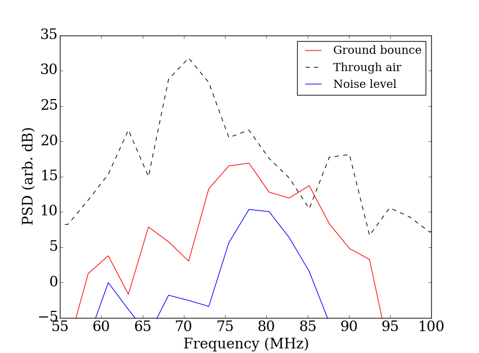
Figure 4: The power spectral density of the received ground bounce signal compared to the noise level in the trace. The power spectral density of the through-air normalization signal, with 40 dB of additional attenuation compared to the ground bounce signal, is shown for comparison with a dashed line. All data have been filtered (65-85 MHz), time-windowed, and zero-padded in the same way (see the text for more details).

Figure 4 shows the time-windowed power spectral density of the ground bounce in red, time-windowed on the red region (200 ns) in Figure 2, filtered to 65-85 MHz using a Butterworth filter of order three, and zero-padded in the time domain. The blue line in Figure 4 shows the typical noise level in the trace taken from a typical (noise-only) time window well after the observed ground bounce in time. It has been time-windowed, filtered, and zero-padded in the same way as the ground bounce signal region.

To measure the radio-frequency loss observed through the ice, we compare the power in the received ground bounce signal to the power in the signal measured through the air with the same setup but with the antennas 46 m apart and aimed directly toward each other. We use this method because the response of our system cancels out in the normalization between the ground bounce and the direct through-air signal. Figure 5 shows the waveform of the normalization signal transmitted directly through the air, filtered to 65-85 MHz in the same way as the ground bounce signal, and with an additional 40 dB attenuator inserted before the low-noise amplifier compared to the sketch in Figure 1. The power spectral density for the through-air normalization signal, with 40 dB of additional attenuation compared to the ground bounce signal, is shown with a dashed line in Figure 4. It has been time-windowed, filtered, and zero-padded in the same way as the ground bounce signal region.

From the ground bounce signal power, we subtract the power spectral density of the typical noise region shown in Figure 4. We process the through-air signal in the same way as the ground bounce and noise traces, producing a power spectral density of the through-air signal that is time-windowed, filtered, and zero-padded in the same way as the ground bounce. We then integrate the power between 65-85 MHz in the noise-subtracted ground bounce and the through-air signal. Using the square root of the total integrated power in this frequency range for $V_{ice}$ and $V_{air}$ and accounting for the 40 dB of additional attenuation on the receiver, we calculate the depth-averaged field attenuation length through the ice using Equation 3. We assume the power reflection coefficient $R$ to be 0.3, which is typical of the ice-bedrock interface (?), and the antenna transmission ratio $T_{\mathrm{ratio}}$ to be 1.0, which was the measured value at 75 MHz for similar antennas by ? on the Ross Ice Shelf. We calculate that $\langle L_{\alpha}\rangle=947$ m at 75 MHz.

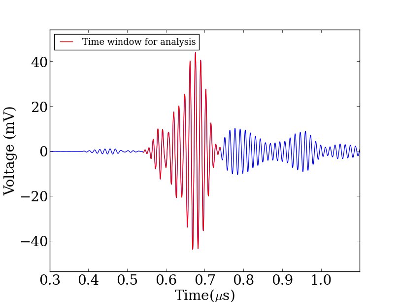
Figure 5: The transmitted impulsive signal received directly through 46 m of air, Butterworth filtered to 65-85 MHz. The system used is the same as for the ground bounce, but with 40 dB of additional attenuation on the receiver. The red region shows the time window used for analysis (200 ns wide).

2.3 Systematic Errors

Index of Refraction: One error on the attenuation length measurement comes from the uncertainty in the assumed index of refraction of ice, which translates linearly to an uncertainty on the distance to the ground bounce. The index of refraction of glacial ice has been measured to be temperature independent in the measured temperature range of the ice at Summit Station with $n=1.78\pm 0.03$ by ?, corresponding to an uncertainty on the depth of the ice of $3014^{+48}_{-50}$ m and on $\langle L_{\alpha}\rangle$ of ${}^{+18}_{-18}$ m.

Antenna Coupling: The transmission coefficient ($\mathrm{S}_{21}$) of the antennas changes when the antennas are coupled to the ice compared to when they are coupled to the air. We made measurements of the reflection coefficient ($\mathrm{S}_{11}$) for these antennas in the field (shown in Figure 3). Assuming that all power that is not reflected is transmitted, the antennas transmit over 98% of the power in the frequency range of interest for the analysis (65-85 MHz) both when coupled to ice and coupled to air, indicating that $T_{\mathrm{ratio}}=1.0$. We also use direct measurements of the transmission properties of similar antennas made by ?, which indicate a value of $T_{\mathrm{ratio}}=1.0$ at 75 MHz, with an uncertainty of about 10%. We include this 10% uncertainty in the power transmitted due to the different coupling to the air and snow of the log-periodic antennas ($T_{\mathrm{ratio}}$). This corresponds to an uncertainty on $\langle L_{\alpha}\rangle$ of ${}^{+14}_{-16}$ m.

Power Reflection Coefficient: The power reflection coefficient at the ice-rock interface is not well known. In our calculation, we assume a power reflection coefficient of 0.3, which is typical of a bedrock-ice interface. Table 1 shows the effect on field attenuation length for different assumptions on the power reflection coefficient. Assuming a perfect reflector at the bottom ($R=1$) is a conservative assumption, and yields a shorter attenuation length. We take the uncertainty on $\langle L_{\alpha}\rangle$ to be ${}^{+89}_{-82}$ m: the range of field attenuation lengths derived using a power reflection coefficient of $R=0.1$ to $R=1.0$.

Power Reflection Coefficient	Field Attenuation Length $\langle L_{\alpha}\rangle$
0.1	1038 m
0.3	947 m
1.0	865 m
1.25	853 m

Table 1: The depth-averaged electric field attenuation length as a function of the choice of power reflection coefficient at the ice-bedrock interface. We include a calculation with $R$=1.25, an extremely pessimistic case that would require magnification effects at the ice-bedrock interface.

Other Possible Sources of Error: Other possible sources of uncertainty include uncertainty in the density profile of the firn, the effect of birefringence in the ice, the effect of any physical bedrock features, and any change in gain of the antennas when coupled directly to the snow. The effect of the first on our measurement is small.

Birefringence has been shown in general to cause losses as large as 10 dB in our frequency range, but it is suspected that the loss due to birefringence is much smaller at places along an ice sheet divide such as the Summit Station site (?). This is due to the lack of strong horizontal preference in the ice crystal fabric because of slow ice flow and is evidenced by previous measurements at the site (?). We plan to make further measurements of the effect of birefringence on the measured attenuation length at the Summit Station site.

Features at the bedrock surface could serve to either magnify or demagnify the reflected signal, depending on the geometry of the surface. Our calculation assumes that the signal is reflected off of a flat, horizontal surface and suffers no magnification effects. This is a good approximation of the ice-bedrock layer around the Summit Station site, which does not have dramatic features at the bedrock surface (?).

Since the frequency response of the antennas shifts lower in frequency by $\sim 20\%$ when the antennas are placed in the snow (see Figure 3), the beam pattern at a given frequency in snow corresponds to a beam pattern at a $\sim 20\%$ higher frequency in air. For log-periodic antennas, we do not expect the gain to be dramatically different over the frequency range of interest, so the contribution to the total error is subdominant.

Total Error: Combining all of the quantifiable uncertainties (antenna coupling, index of refraction, and reflection coefficient), we find a the total uncertainty on $\langle L_{\alpha}\rangle$ of ${}^{+92}_{-85}$ m:

2.4 Results

We have calculated the depth-averaged electric field attenuation length at 75 MHz through an analysis of the ground bounce measurement, and have quantified the systematic errors associated with the measurement. We find the depth-averaged attenuation length including all quantifiable uncertainties to be $\langle L_{\alpha}\rangle=947^{+92}_{-85}$ m at 75 MHz.

3 Discussion and Summary

We combine our measurement of the depth-averaged field attenuation length $\langle L_{\alpha}\rangle$ with the measured temperature profile of the ice at the Summit Station Site from the GRIP borehole (??) and the measured dependence of attenuation length on temperature from ? (shown in Figure 6) to extract a profile of attenuation length as a function of depth. For the dependence of attenuation length on temperature, we assume the average slope of the two locations on which ? report, shown as the blue line in Figure 6. The field attenuation length as a function of depth is shown in Figure 7. The average field attenuation length over the upper 1500 m, from where the vast majority of the neutrino events that a surface or sub-surface radio detector could detect would originate, is $\langle L_{\alpha}\rangle$=$1149^{+112}_{-103}$ m at 75 MHz.

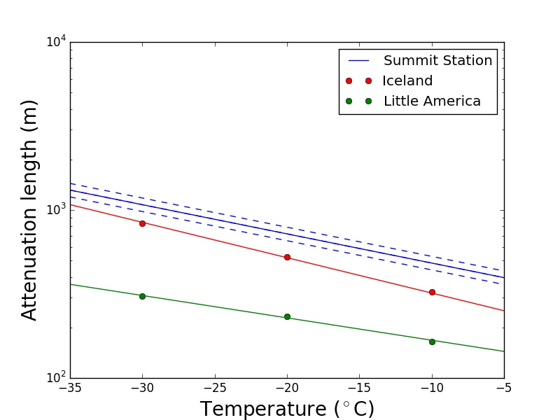
Figure 6: The electric field attenuation length as a function of temperature for the Summit Station site, shown with the blue line. We have assumed that the relationship between attenuation length and temperature is consistent with the measured attenuation length vs. temperature from ?, also shown on this plot (red and green lines). The dashed lines denote $\pm 1\sigma$.

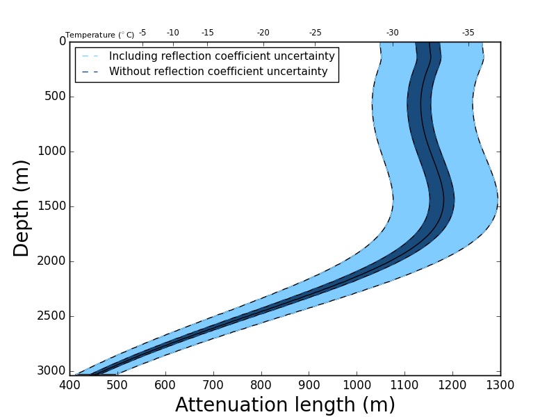
Figure 7: The extracted electric field attenuation length profile as a function of depth for the Summit Station site at 75 MHz. We have combined our measurements with the temperature profile measured for the GRIP borehole (??) and the measured attenuation length vs. temperature from ?. The shaded region denotes $\pm 1\sigma$. We have not included a firn density correction, which would be a small effect.

To compare with measurements made at the South Pole and on the Ross Ice Shelf, we extrapolate our results to 300 MHz (???). This is a model-dependent extrapolation. We use an ensemble of measurements of the attenuation length as a function of frequency of glacial ice from Antarctica, Iceland, and Greenland (??) and (Westphal cited in (?)) to perform a linear extrapolation. We take the average of the best and worst cases from this ensemble, yielding a linear extrapolation with a slope of $-0.55$ m/MHz. This yields an estimate of the field attenuation length in the top 1500 m at 300 MHz of $1022^{+230}_{-253}$ m. We note that this extrapolation introduces a large uncertainty (reflected in the error bars quoted) because the properties of glacial ice at different locations are variable, and a direct measurement at Summit Station at higher frequencies would be more robust. We take the additional uncertainty to be the scatter in the measurements of attenuation length as a function of frequency.

We also took data in a similar experimental configuration with Seavey broadband quad-ridged horn antennas from Antenna Research Associates that are sensitive between 200-1200 MHz. The experimental setup that we used for these higher frequencies did not have enough sensitivity make a direct measurement at 300 MHz due to a smaller antenna effective area and less power in the broadband high-voltage pulser. However, as a consistency check, we can place an upper limit on the depth-averaged attenuation length at 300 MHz from the higher-frequency data. Following the same procedure outlined previously, but at 300 MHz, we calculate that our system was sensitive to a depth-averaged attenuation length of 1100 m or longer at 300 MHz. Applying the frequency extrapolation described in this Section to the measured depth-averaged attenuation length $\langle L_{\alpha}\rangle$ of $947^{+92}_{-85}$ m at 75 MHz yields a depth-averaged attenutation length at 300 MHz of $823^{+189}_{-209}$ m, consistent with our directly-derived upper limit.

We compare the results of our measurement and extrapolation of the field attenuation length at Summit Station in the top 1500 m at 300 MHz of $1022^{+230}_{-253}$ m with other in situ measurements of radio attenuation at possible sites for neutrino detectors. For deep sites, we follow the convention established by ? and compare the attenuation length in the top 1500 m of the ice, since that is where the vast majority of neutrino events that a surface or sub-surface detector occur. For the site on the Ross Ice Shelf, we use the depth-averaged attenuation length, since the total depth of the ice is much less than 1500 m. At 300 MHz, the radio attenuation length measured on the Ross Ice Shelf (?) is $\langle L_{\alpha}\rangle=411$ m with an experimental uncertainty of about 40 m averaged over all depths for the 578 m thick ice. This measurement has been redone recently, with a consistent result (?). The attenuation length at the South Pole has been measured to be $\langle L_{\alpha}\rangle=1660^{+255}_{-120}$ m for the top 1500 m (?). The longer attenuation length at the South Pole in the upper 1500 m compared to Summit Station can mainly be attributed to the fact that the ice is colder in the upper 1500 m ($\sim-50^{\circ}$C at the South Pole compared to $\sim-30^{\circ}$C at the Summit Station site).

Our measurement of radio-frequency attenuation length at Summit Station is 25% longer than the comparison that we can make to the previously measured South Pole attenuation length (?), after accounting for the difference in temperature profiles between the South Pole and Summit Station and assuming the relationship between attenuation length and temperature as described above and from ?. This is not meant to be an exact prediction, but rather a comparison of the ice after removing obvious differences such as temperature and depth. Our measurement is also consistent with recent radar measurements of attenuation length at 195 MHz across the Greenland Ice Sheet, including near Summit Station (?).

The Summit Station site is an appealing choice to host a detector for UHE neutrinos. The site sits on top of the deepest part of the roughly 3 km deep Greenland ice sheet, providing a huge detection volume. The radio attenuation length of the ice is comparable to sites in the Antarctic. The development of a northern site for UHE neutrino detection will allow for different sky coverage compared to developing Antarctic arrays (??).

4 Acknowledgements

We would like to thank CH2MHill and the US National Science Foundation (NSF) for the dedicated, knowledgeable, and extremely helpful logistical support team, particularly to K. Gorham. We are deeply indebted to those who dedicate their careers to help make our science possible in such remote environments. This work was supported by the NSF’s Office of Polar Programs (PLR-1103553), the US Department of Energy, the Kavli Institute for Cosmological Physics at the University of Chicago, the University of California, Los Angeles, and the Illinois Space Grant Consortium. We would like to thank P. Gorham for support of C. Miki. We would also like to thank Warner Brothers Studios for lending us parkas for the expedition.

Bibliography

- Allison P and others (2012) Design and initial performance of the Askaryan Radio Array prototype EeV neutrino detector at the South Pole. Astroparticle Physics, 35, 457–477 (10.1016/j.astropartphys.2011.11.010)
- Arthern RJ and others (2013) Inversion for the density-depth profile of polar firn using a stepped-frequency radar. Journal of Geophysical Research (Earth Surface), 118, 1257–1263 (10.1002/jgrf.20089)
- Askaryan G (1962) Excess negative charge of an electron-photon shower and its coherent radio emission. Soviet Physics JETP, 14, 441–442
- Bamber JL, Layberry RL and Gogineni SP (2001) A new ice thickness and bed data set for the greenland ice sheet: 1. measurement, data reduction, and errors. Journal of Geophysical Research: Atmospheres (1984–2012), 106(D24), 33773–33780 (10.1029/2001JD900053)
- Barrella T, Barwick S and Saltzberg D (2011) Ross Ice Shelf (Antarctica) in situ radio-frequency attenuation. Journal of Glaciology, 57, 61–66 (10.3189/002214311795306691)
- Barwick S and others (2005) South Polar in situ radio-frequency ice attenuation. Journal of Glaciology, 51, 231–238 (10.3189/172756505781829467)
- Besson DZ and others (2008) In situ radioglaciological measurements near Taylor Dome, Antarctica and implications for ultra-high energy (UHE) neutrino astronomy. Astroparticle Physics, 29, 130–157 (10.1016/j.astropartphys.2007.12.004)
- Bogorodsky VV, Bentley CR and Gudmandsen P (1985) Radioglaciology. Reidel Publishing Co. (10.1007/978-94-009-5275-1)
- Gorham P and others (2007) Observations of the Askaryan Effect in Ice. Physical Review Letters, 99(17), 171101 (10.1103/PhysRevLett.99.171101)
- Gorham P and others (2009) The Antarctic Impulsive Transient Antenna ultra-high energy neutrino detector: Design, performance, and sensitivity for the 2006-2007 balloon flight. Astroparticle Physics, 32, 10–41 (10.1016/j.astropartphys.2009.05.003)
- Greenland Ice Core Project (1994) ftp://ftp.ncdc.noaa.gov/ pub/data/paleo/icecore/greenland/summit/grip/physical/ griptemp.txt
- Halzen F, Zas E and Stanev T (1991) Radiodetection of cosmic neutrinos. a numerical, real time analysis. Physics Letters B, 257(3), 432–436 (10.1016/0370-2693(91)91920-Q)
- Hanson JC and others (2015) Radar absorption, basal reflection, thickness, and polarization measurements from the Ross Ice Shelf, Antarctica. Journal of Glaciology, 61(227) (doi:10.3189/2015JoG14J214)
- Hoffman K and others (2007) AURA: The Askaryan Underice Radio Array. Journal of Physics Conference Series, 81(1), 012022 (10.1088/1742-6596/81/1/012022)
- Jiracek G (1967) Radio sounding of Antarctic ice. Univ. Wisconsin Geophys. Polar Res. Center Res. Rep. Ser., 67
- Johnsen SJ, Dahl-Jensen D, Dansgaard W and Gundestrup N (1995) Greenland palaeotemperatures derived from grip bore hole temperature and ice core isotope profiles. Tellus B, 47(5), 624–629 (10.1034/j.1600-0889.47.issue5.9.x)
- Klein SR and others (2013) A Radio Detector Array for Cosmic Neutrinos on the Ross Ice Shelf. IEEE Transactions on Nuclear Science, 60, 637–643 (10.1109/TNS.2013.2248746)
- Kovacs A, Gow A and Morey R (1995) The in-situ dielectric constant of polar firn revisited. Cold Regions Science and Technology, 23, 245–256 (10.1016/0165-232X(94)00016-Q)
- Kravchenko I and others (2003) Performance and simulation of the RICE detector. Astroparticle Physics, 19, 15–36 (10.1016/S0927-6505(02)00194-9)
- MagGregor JA and others (2015) Radar attenuation and temperature within the Greenland Ice Sheet. J. Geophys. Res. Earth Surf., 120, 983–1008 (doi:10.1002/2015JF003418)
- Paden J and others (2005) Wideband measurements of ice sheet attenuation and basal scattering. IEEE Geoscience and Remote Sensing Letters, 2 (10.1109/LGRS.2004.842474)
- Saltzberg D and others (2001) Observation of the Askaryan Effect: Coherent Microwave Cherenkov Emission from Charge Asymmetry in High-Energy Particle Cascades. Physical Review Letters, 86, 2802 (10.1103/PhysRevLett.86.2802)
- Walford MER (1968) Field measurements of dielectric absorption in Antarctic ice and snow at very high frequencies. Journal of Glaciology, 7, 89–94