PMU based Detection of Imbalance in Three-Phase Power Systems

Abstract

The problem of imbalance detection in a three-phase power system using a phasor measurement unit (PMU) is considered. A general model for the zero, positive, and negative sequences from a PMU measurement at off-nominal frequencies is presented and a hypothesis testing framework is formulated. The new formulation takes into account the fact that minor degree of imbalance in the system is acceptable and does not indicate subsequent interruptions, failures, or degradation of physical components. A generalized likelihood ratio test (GLRT) is developed and shown to be a function of the negative-sequence phasor estimator and the acceptable level of imbalances for nominal system operations. As a by-product to the proposed detection method, a constrained estimation of the positive and negative phasors and the frequency deviation is obtained for both balanced and unbalanced situations. The theoretical and numerical performance analyses show improved performance over benchmark techniques and robustness to the presence of additional harmonics.

I Introduction

The three-phase power system is designed to operate at a nominal frequency in a near-balanced fashion [1]. In practice, frequency deviation and load imbalance are the norm rather than the exception. According to the American National Standards Institute (ANSI) report [2], $2\%$ of the electrical distribution systems in USA have a significant undesirable degree of imbalance, leading to several serious consequences. First, frequency deviations and imbalances may be a precursor to more serious contingencies leading to possible blackouts [3], [4]. In addition, substantial power imbalance causes excessive losses, overheating, insulation degradation, a reduced lifespan of motors and transformers, and interruptions in production processes [5, 6, 7, 8].

Thus, the ability to detect potentially harmful levels of imbalance in various power systems is highly desirable for the benefit of both the utility and customer [4], [6]. However, in most phasor measurement applications it is common and acceptable [2] to have some degree of imbalance in the system due to unbalanced loads and untransposed transmission lines [1]. To this end, effective algorithms and sophisticated methods are crucial for estimating frequency deviations and phasors in the event of system imbalance and detecting an abnormal level of imbalance. It is in this context that modern sensing devices, such as phasor measurement units (PMUs), have the potential to provide rapid detection of contingencies and situational awareness (see [1] and references therein).

I-A Summary of results

In this paper we consider detection of voltage imbalance in three-phase power systems using the native frequency output of PMU. The contribution of the paper is threefold. First, we develop a statistical model that captures characteristics of imbalance from PMU output. In particular, we provide the noise statistics and demonstrate that, for a perfectly balanced power system, the PMU output is a single complex sinusoid, whereas, under imbalance, the symmetrical components at the PMU output have two related frequencies. The statistical model indicates that, at the nominal frequency, imbalance is undetectable by using only the positive-sequence. Therefore, detection of imbalance should be carried out by using the negative-sequence and/or the zero-sequence in addition to the positive-sequence. Second, we derive a hypothesis testing technique based on the principle of generalized likelihood ratio test (GLRT). The proposed GLRT uses the constrained maximum-likelihood (CML) estimators of the frequency deviation and the three symmetrical component phasors under the balanced and unbalanced system operating conditions. Third, we analyze the performance of the proposed GLRT and provide simulation results in practical settings. In particular, in Section IV, we present an analysis of false alarm probability from which we obtain a practical way of setting detection thresholds for given false alarm probabilities. Simulations studies are presented in Section V, where we demonstrate the performance of the proposed GLRT for single-phase magnitude and phase imbalances. We demonstrate that at high signal-to-noise ratios (SNR), the GLRT with estimated frequency coincides with the known-frequency GLRT and thus, the frequency estimation has no impact in this region. Of particular importance is the evaluation of the robustness of the proposed algorithm in the presence of higher-order harmonics. We show that the probability of detection of the GLRT for non-sinusoidal voltages is close to those of the sinusoidal case. Therefore, the proposed method can also be used in the presence of inter-harmonics.

I-B Related works

Under perfectly balanced three-phase operating conditions, the zero and negative sequences are absent, hence the state-estimation and signal analysis in this case are carried out using only the positive-sequence model [3, 9]. When system imbalance occurs, the zero and negative sequences are nonzero, and the PMU’s output exhibits nonstationary frequency deviations [4], [10]. In addition, the positive-sequence measurements become non-circular as described in [11], [12]. In the pioneering works of [11] and [12], new methods were derived for frequency-estimation based on non-circular models and the Clarke’s transformation. These methods use the positive and negative sequences and analyze the measurements in the time domain. The mismatch estimation error caused by using the balanced state estimation under imbalance is studied in [3] and the influence of imperfect synchronization on the state estimation is described in [13]. In [14] a distribution system state estimator suitable for monitoring unbalanced distribution networks is presented. A practical procedure to decrease the state estimation error introduced by load imbalances is developed in [15].

In the literature, various definitions are given for imbalance in a power system, where the fundamental performance measures are the voltage unbalance factor (VUF) [4], [16], [17] and the percent voltage unbalance (PVU) [18]. The VUF is the ratio of the magnitudes of negative- and positive-sequence voltages and the PUV is equal to the ratio of the maximum voltage magnitude deviation of the zero, positive, and negative sequences from the average of the three-phase voltage magnitudes [19]. The phase angle imbalance, which is not reflected in either the VUF or PVU measures, can be described by the phase voltage unbalance factor (PVUF) [20] and the complex VUF (CVUF) [21], [22]. The limitations of these commonly-used methods can be found, for example, in [23]. An online identification method of the level, location, and effects of voltage imbalance in a distribution network is derived in [6] based on distribution system state estimation. However, the existing non-parametric methods for detection of imbalance are insufficient (e.g., [23, 21, 22, 24]). Derivation of parametric detection methods is expected to improve the detection performance.

A particularly relevant prior work is [25] where the authors develop the first parametric GLRT for detecting voltage and phase imbalances based on time domain measurements. While [25] and this paper both use GLRT principle, the models considered and the statistics used are quite different. Specifically, the approach presented here is based on the native PMU (frequency domain) output that is less informative than the time domain measurements used in [25] but more readily accessible. More significance, perhaps, is the formulation of hypotheses. The GLRT derived in [25] tests the hypothesis that the system is perfectly balanced against any amount of imbalance in the system. Our approach, on the other hand, aims to detect substantial imbalance. The presence of imbalance in the null hypothesis (the nominal case) presents nontrivial technical difficulties, which cannot be dealt with by simply changing the detection threshold on a test designed for a perfectly balanced system operating at the nominal frequency. Finally, since usually the zero-sequence power does not propagate to the machine terminals [4], [26, 27, 28], the information which is used by the proposed GLRT includes only the positive and negative sequence components, while [25] uses the three sequences and investigates the influence of the zero sequence on the detection performance.

In most situations, frequency deviations and minor imbalances can be mitigated by frequency regulation or load compensation techniques [29]. In the literature, several mitigation techniques have been suggested to correct significant voltage imbalance problems [4], on both the power system and user facility levels. Voltage imbalance is ultimately fixed by manually or automatically rebalancing loads and removing asymmetric network line configurations [6], where these are costly processes and inappropriate for frequent but small imbalances. For example, the compensation of the voltage imbalance can be achieved by reducing the negative-sequence voltage using a series active power filter or based on shunt compensation, as described in [30], or by advanced control strategies [31, 32, 33]. In addition, the compensation of voltage harmonics, which can be generated by a nonlinear unbalanced load, can be considered by separating the positive and negative sequences of each harmonic order [30].

Nomenclature

$V_{a},V_{b},V_{c}$ Three-phase voltage magnitudes $\varphi_{a},\varphi_{b},\varphi_{c}$ Three-phase voltage phases ${\bf{v}}$ $\left[V_{a}e^{j\varphi_{a}},V_{b}e^{j\varphi_{b}},V_{c}e^{j\varphi_{c}}\right]^{\mbox{\tiny T}}$ $\omega_{0}$ Nominal grid-frequency $\Delta$ Frequency deviation $\hat{\Delta}^{(i)}$ ML frequency-deviation estimator under hypothesis $i=0,1$ $\hat{\Delta}_{s}$ Suboptimal frequency-deviation estimator $N$ Samples per cycle at time domain $K$ Samples at the frequency domain $v_{a}[n],v_{b}[n],v_{c}[n]$ Three-phase voltages at time $n$ $V_{0}[k],V_{+}[k],V_{-}[k]$ Frequency domain zero, positive, and negative phasor sequences at time $k$ ${\bf{w}}_{a,b,c}[n]$ Gaussian noise sequences at time $n$ $W_{0}[k],W_{+}[k],W_{-}[k]$ Complex Gaussian noise sequences at frequency-time $k$ $\sigma^{2}$ Noise variance ${\bf{I}}_{K}$ $K\times K$ identity matrix ${\mathbf{1}}_{K}$ Vector of ones of size $K$ $\alpha$ $e^{j2\pi/3}$ $\gamma$ $\frac{2\pi}{N}$ $C_{0},C_{+},C_{-}$ Zero, positive, and negative phasors $\hat{C}_{+}^{(i)},\hat{C}_{-}^{(i)}$ Positive and negative phasor CML estimators under hypothesis $i$ $\hat{C}_{-}^{(uc)}$ Negative phasor ML estimator $\tilde{{\mbox{\boldmath$\nu$}}}_{0},\tilde{{\mbox{\boldmath$\nu$}}}_{+},\tilde{{\mbox{\boldmath$\nu$}}}_{-}$ PMU’s measurement vectors ${\mbox{\boldmath$\nu$}}_{0},{\mbox{\boldmath$\nu$}}_{+},{\mbox{\boldmath$\nu$}}_{-}$ Whitened PMU’s measurement vectors $\theta$ Unknown parameters vector $L({\mbox{\boldmath$\theta$}})$ Likelihood function at $\theta$ $T_{\text{GLRT}}$ GLRT detector $T_{\text{GLRT-SNH}}$ GLRT-SNH detector $T_{\text{VUF}}$ VUF detector $\tau$ Detector’s threshold $P_{e}(\tau)$ GLRT false alarm probability at $\tau$ $P_{e}^{(a)}(\tau)$ False alarm asymptotic probability at $\tau$ $r$ Authorized level of imbalances.

I-C Organization and notations

The remainder of the paper is organized as follows: Section II presents the mathematical model and outlines several special cases. The GLRT detector and CML estimators for detecting imbalance are derived in Section III. In Section IV, a performance analysis of the proposed GLRT is developed. Finally, the proposed method is evaluated via simulations in Section V and the conclusion appear in Section VI.

In the rest of this paper we denote vectors by boldface lowercase letters and matrices by boldface uppercase letters. The operators $(\cdot)^{*}$, $(\cdot)^{\mbox{\tiny$T$}}$, $(\cdot)^{\mbox{\tiny$H$}}$, and $(\cdot)^{-1}$ denote the complex conjugate, transpose, Hermite, and inverse operators, respectively. The operator ${\text{Real}}\{\cdot\}$ denotes the real part of its argument. For convenience, variables are cataloged in the Nomenclature Table.

II Measurement model

The system and measurement models considered here are conventional (see, e.g., [1, 10]). In this section we present the model in a statistical signal processing formulation that includes a description of the noise statistics, and it is more convenient for developing estimation and detection algorithms [34]. In particular, we describe the statistical behavior of the PMU output, i.e. after the sampling, symmetrical transformation, and nominal-frequency discrete Fourier transform (DFT) operation.

II-A Off-nominal unbalanced system phasors

The voltages in a three-phase power system are assumed to be pure sinusoidal signals of frequency $\omega_{0}+\Delta$, where $\omega_{0}$ is the known nominal-frequency ($100\pi$ or $120\pi$) and $\Delta$ is the frequency deviation from this nominal value. The magnitudes and phases of the three voltages are denoted by $V_{a},V_{b},V_{c}\geq 0$ and $\varphi_{a},\varphi_{b},\varphi_{c}\in[0,2\pi]$, respectively. The three-phase power system is balanced or symmetrical if $V_{a}=V_{b}=V_{c}$ and $\varphi_{a}=\varphi_{b}+\frac{2\pi}{3}=\varphi_{c}-\frac{2\pi}{3}$. The PMU samples these real signals $N$ times per cycle of the nominal-frequency, $\omega_{0}$, to produce the following discrete-time, noisy measurements model (e.g. [1], pp. 51-52 and [35]):

$$\left[\begin{array}[]{c}v_{a}[n]\\ v_{b}[n]\\ v_{c}[n]\end{array}\right]=\left[\begin{array}[]{c}V_{a}\cos\left(\gamma\frac{\omega_{0}+\Delta}{\omega_{0}}n+\varphi_{a}\right)\\ V_{b}\cos\left(\gamma\frac{\omega_{0}+\Delta}{\omega_{0}}n+\varphi_{b}\right)\\ V_{c}\cos\left(\gamma\frac{\omega_{0}+\Delta}{\omega_{0}}n+\varphi_{c}\right)\end{array}\right]+{\bf{w}}_{a,b,c}[n]\hskip 2.84544pt$$ (7)

$$={\text{Real}}\left\{e^{j\gamma\frac{\omega_{0}+\Delta}{\omega_{0}}n}{\bf{v}}\right\}+{\bf{w}}_{a,b,c}[n]\hskip 54.06006pt$$

$$=\frac{1}{2}e^{j\gamma\frac{\omega_{0}+\Delta}{\omega_{0}}n}{\bf{v}}+\frac{1}{2}e^{-j\gamma\frac{\omega_{0}+\Delta}{\omega_{0}}n}{\bf{v}}^{*}+{\bf{w}}_{a,b,c}[n],$$ (8)

for all $n\in{\mathbb{Z}}$, where $\gamma\stackrel{{\scriptstyle\triangle}}{{=}}\frac{2\pi}{N}$ and ${\bf{v}}\stackrel{{\scriptstyle\triangle}}{{=}}\left[V_{a}e^{j\varphi_{a}},V_{b}e^{j\varphi_{b}},V_{c}e^{j\varphi_{c}}\right]^{\mbox{\tiny T}}$. The noise sequence, $\{{\bf{w}}_{a,b,c}[n]\}_{n\in{\mathbb{R}}}$, is assumed to be a real white Gaussian noise sequences with known covariance matrix $\sigma^{2}{\bf{I}}_{3}$. The derived method can be easily extended to the more general case of a correlated three-phase system [6] by using a non-diagonal covariance matrix. The error covariance matrix can be obtained, for example, as described in [6].

The PMU constructs the complex representation of the signals by using a DFT operator over one cycle of the nominal-frequency [1], [10]. That is, the PMU DFT operation on any arbitrary signal $x[n]$ results in the following phasor sequence:

$$X[k]=\frac{\sqrt{2}}{N}\sum_{n=k}^{k+N-1}x[n]e^{-j\gamma n},~{}~{}~{}k=0,\ldots,K-1,$$ (9)

where the index $k$ refers to the beginning of the DFT window. By substituting the three sequences, $v_{a}[n]$, $v_{b}[n]$, and $v_{c}[n]$, for all $n\in{\mathbb{Z}}$ from (7) in (9). Using the identity [36],

$$\sum_{n=k}^{k+N-1}e^{j\alpha n}=\frac{\sin(\alpha N/2)}{\sin(\alpha/2)}e^{j\alpha\left(k+\frac{N-1}{2}\right)},~{}\forall\alpha\in{\mathbb{R}},$$

we obtain the following phasor sequences measurements:

$$\left[\begin{array}[]{c}V_{a}[k]\\ V_{b}[k]\\ V_{c}[k]\end{array}\right] = \frac{\sqrt{2}}{N}\left[\begin{array}[]{c}\sum_{n=k}^{k+N-1}v_{a}[n]e^{-j\gamma n}\\ \sum_{n=k}^{k+N-1}v_{b}[n]e^{-j\gamma n}\\ \sum_{n=k}^{k+N-1}v_{c}[n]e^{-j\gamma n}\end{array}\right]$$ (17)

$$= \frac{1}{\sqrt{2}}Pe^{j\gamma\frac{\Delta}{\omega_{0}}k}{\bf{v}}+\frac{1}{\sqrt{2}}Qe^{-j\gamma\frac{2\omega_{0}+\Delta}{\omega_{0}}k}{\bf{v}}^{*}$$

$$+\frac{\sqrt{2}}{N}\sum_{n=k}^{k+N-1}{\bf{w}}_{a,b,c}[n]e^{-j\gamma n},$$

$k=0,\ldots,K-1$, where

$$P = \frac{\sin(\gamma N\frac{\Delta}{2\omega_{0}})}{N\sin(\gamma\frac{\Delta}{2\omega_{0}})}e^{j\gamma\frac{\Delta}{\omega_{0}}\frac{N-1}{2}}$$ (18)

$$Q = \frac{\sin(\gamma N\frac{2\omega_{0}+\Delta}{2\omega_{0}})}{N\sin(\gamma\frac{2\omega_{0}+\Delta}{2\omega_{0}})}e^{-j\gamma\frac{2\omega_{0}+\Delta}{\omega_{0}}\frac{N-1}{2}}.$$ (19)

It is seen, then, that $P$ and $Q$ are functions of the unknown frequency deviation, $\Delta$, but independent of $k$.

Finally, the three symmetrical voltage sequences are calculated from three-phase voltages by the PMU using the symmetrical component transformation (e.g. [1] pp. 63-67):

$$\left[\begin{array}[]{c}V_{0}[k]\\ V_{+}[k]\\ V_{-}[k]\end{array}\right]=\frac{1}{3}\underbrace{\left[\begin{array}[]{ccc}1&1&1\\ 1&\alpha&\alpha^{2}\\ 1&\alpha^{2}&\alpha\end{array}\right]}_{\stackrel{{\scriptstyle\triangle}}{{=}}{\bf{H}}}\left[\begin{array}[]{c}V_{a}[k]\\ V_{b}[k]\\ V_{c}[k]\end{array}\right],$$ (20)

for all $k=0,1,\ldots,K-1$, where $V_{0}[k],V_{+}[k]$, and $V_{-}[k]$ are the zero, positive, and negative sequences, respectively, and $\alpha=e^{j2\pi/3}$. By substituting (17) in (20), we obtain

$$V_{0}[k]=Pe^{j\gamma\frac{\Delta}{\omega_{0}}k}C_{0}+Qe^{-j\gamma\frac{2\omega_{0}+\Delta}{\omega_{0}}k}C_{0}^{*}+W_{0}[k]$$ (21)

$$V_{+}[k]=Pe^{j\gamma\frac{\Delta}{\omega_{0}}k}C_{+}+Qe^{-j\gamma\frac{2\omega_{0}+\Delta}{\omega_{0}}k}C_{-}^{*}+W_{+}[k]$$ (22)

$$V_{-}[k]=Pe^{j\gamma\frac{\Delta}{\omega_{0}}k}C_{-}+Qe^{-j\gamma\frac{2\omega_{0}+\Delta}{\omega_{0}}k}C_{+}^{*}+W_{-}[k]$$ (23)

$k=0,\ldots,K-1$, where

$$\left[C_{0},C_{+},C_{-}\right]^{T}=\frac{\sqrt{2}}{6}{\bf{H}}{\bf{v}}$$

and

$$\left[W_{0}[k],W_{+}[k],W_{-}[k]\right]^{\mbox{\tiny$T$}}=\frac{\sqrt{2}}{3N}{\bf{H}}\sum_{n=k}^{k+N-1}{\bf{w}}_{a,b,c}[n]e^{-j\gamma n},$$

for all $k=0,\ldots,K-1$. Since ${\bf{H}}{\bf{H}}^{\mbox{\tiny$H$}}=3{\bf{I}}_{3}$, the noise sequences, $W_{0}[k]$, $W_{+}[k]$, $W_{-}[k]$, $k=1,\ldots,K-1$, are independent complex circularly symmetric Gaussian noise sequences where each sequence has a variance of $\frac{2\sigma^{2}}{3N}$. However, it should be noted that if the original three-phase noise signals are correlated, which is the case in distribution systems [6], [37], then, the noise sequences of the three symmetrical components are also correlated. It can be seen that the PMU output in (21)-(23) includes samples of the symmetrical sequences, $W_{0}[k],W_{+}[k],W_{-}[k]$, at the nominal-frequency bin, that are different from the true value of the input sequence phasors, $C_{0}$, $C_{+}$, and $C_{-}$.

In this work, we are interested in the detection of imbalances based on $K$ measurements of the positive and negative sequences from (21)-(23). The PMU output of the zero sequence, $V_{0}[0],\ldots,V_{0}[K-1]$ is usually non observable and is described in this paper for the sake of completeness. The models for these $K$ measurements can be written in matrix form as follows:

$$\tilde{{\mbox{\boldmath$\nu$}}}_{0} = PC_{0}\tilde{{\bf{e}}}_{1}+QC_{0}^{*}\tilde{{\bf{e}}}_{2}+\tilde{{\bf{w}}}_{0}$$ (24)

$$\tilde{{\mbox{\boldmath$\nu$}}}_{+} = PC_{+}\tilde{{\bf{e}}}_{1}+QC_{-}^{*}\tilde{{\bf{e}}}_{2}+\tilde{{\bf{w}}}_{+}$$ (25)

$$\tilde{{\mbox{\boldmath$\nu$}}}_{-} = PC_{-}\tilde{{\bf{e}}}_{1}+QC_{+}^{*}\tilde{{\bf{e}}}_{2}+\tilde{{\bf{w}}}_{-},$$ (26)

where

$$\tilde{{\mbox{\boldmath$\nu$}}}_{0} \stackrel{{\scriptstyle\triangle}}{{=}} [V_{0}[0],\ldots,V_{0}[K-1]]^{T},$$

$$\tilde{{\mbox{\boldmath$\nu$}}}_{+} \stackrel{{\scriptstyle\triangle}}{{=}} [V_{+}[0],\ldots,V_{+}[K-1]]^{T},$$

$$\tilde{{\mbox{\boldmath$\nu$}}}_{-} \stackrel{{\scriptstyle\triangle}}{{=}} [{V}_{-}[0],\ldots,{V}_{-}[K-1]]^{T},$$

$$\tilde{{\bf{e}}}_{1} \stackrel{{\scriptstyle\triangle}}{{=}} \left[1,e^{j\gamma\frac{\Delta}{\omega_{0}}},\ldots,e^{j\gamma\frac{\Delta}{\omega_{0}}(K-1)}\right]^{T},$$

$$\tilde{{\bf{e}}}_{2} \stackrel{{\scriptstyle\triangle}}{{=}} \left[1,e^{-j\gamma\frac{2\omega_{0}+\Delta}{\omega_{0}}},\ldots,e^{-j\gamma\frac{2\omega_{0}+\Delta}{\omega_{0}}(K-1)}\right]^{T}.$$

The vectors in $\tilde{{\bf{e}}}_{1}$ and $\tilde{{\bf{e}}}_{2}$ are identical to the steering vector for a uniform linear array [38]. The noise vectors, $\tilde{{\bf{w}}}_{0}$, ,$\tilde{{\bf{w}}}_{+}$, and $\tilde{{\bf{w}}}_{-}$, are independent zero-mean complex, circularly symmetric, colored Gaussian noise sequences with covariance matrix ${\bf{R}}$, where ${\bf{R}}$ is a $K\times K$ matrix with the following $(k,l)$th element

$$[{\bf{R}}]_{k,l}=\frac{2\sigma^{2}}{3N^{2}}\left\{\begin{array}[]{lr}N-|k-l|&{\text{if }}-N\leq k-l\leq N\\ 0&{\text{otherwise}}\end{array}\right..$$

Since the error covariance matrix is known, the signals in (24)-(26) can be prewhitened. The whitening operation is performed by left-multiplication of the terms in (24)-(26) by ${\bf{R}}^{-\frac{1}{2}}$:

$${\mbox{\boldmath$\nu$}}_{0} = {\bf{R}}^{-\frac{1}{2}}\tilde{{\mbox{\boldmath$\nu$}}}_{0}=PC_{0}{{\bf{e}}}_{1}+QC_{0}^{*}{{\bf{e}}}_{2}+{{\bf{w}}}_{0}$$ (27)

$${\mbox{\boldmath$\nu$}}_{+} = {\bf{R}}^{-\frac{1}{2}}\tilde{{\mbox{\boldmath$\nu$}}}_{+}=PC_{+}{{\bf{e}}}_{1}+QC_{-}^{*}{{\bf{e}}}_{2}+{{\bf{w}}}_{+}$$ (28)

$${\mbox{\boldmath$\nu$}}_{-} = {\bf{R}}^{-\frac{1}{2}}\tilde{{\mbox{\boldmath$\nu$}}}_{-}=PC_{-}{{\bf{e}}}_{1}+QC_{+}^{*}{{\bf{e}}}_{2}+{{\bf{w}}}_{-},$$ (29)

where ${{\bf{e}}_{m}}\stackrel{{\scriptstyle\triangle}}{{=}}{\bf{R}}^{-\frac{1}{2}}\tilde{{\bf{e}}}_{m}$, $m=1,2$. The modified noise vectors, ${{\bf{w}}}_{0}={\bf{R}}^{-\frac{1}{2}}\tilde{{\bf{w}}}_{0}$, ${{\bf{w}}}_{+}={\bf{R}}^{-\frac{1}{2}}\tilde{{\bf{w}}}_{+}$, ${{\bf{w}}}_{-}={\bf{R}}^{-\frac{1}{2}}\tilde{{\bf{w}}}_{-}$ have an identity covariance matrix, ${\bf{I}}_{K}$. Similarly, the prewhitening procedure can be performed for the more general case of a correlated three-phase system, when the three sequences are dependent.

II-B Special cases

II-B1 Perfectly balanced system

For the special case of a perfectly balanced system, the three-phase voltages satisfy $V_{a}=V_{b}=V_{c}$ and $\varphi_{a}=\varphi_{b}+\frac{2\pi}{3}=\varphi_{c}-\frac{2\pi}{3}$. Therefore, it can be verified that for this case $C_{0}=0$, $C_{-}=0$, and the model in (27)-(29) is reduced to

$$\left\{\begin{array}[]{l}{\mbox{\boldmath$\nu$}}_{0}={\bf{w}}_{0}\\ {\mbox{\boldmath$\nu$}}_{+}=PC_{+}{\bf{e}}_{1}+{\bf{w}}_{+}\\ {\mbox{\boldmath$\nu$}}_{-}=QC_{+}^{*}{\bf{e}}_{2}+{\bf{w}}_{-}\end{array}\right..$$ (33)

The model in (33) indicates that for perfectly balanced systems the zero-sequence is a noise-sequence and the positive and negative sequences create sinusoidal signals.

II-B2 Nominal-frequency system

If the input signal is a pure sinusoid at the nominal-frequency, i.e. $\Delta=0$, then, by using (18), (19), and the L’H$\hat{\text{o}}$pital’s rule, it can be seen that $\lim\limits_{\Delta\rightarrow 0}P=1$, $\lim\limits_{\Delta\rightarrow 0}Q=0$, and $\tilde{{\bf{e}}}_{1}={\mathbf{1}}_{K}$. By substituting these terms in (27)-(29), the output of the PMU for the nominal-frequency case is given by

$$\left\{\begin{array}[]{l}{\mbox{\boldmath$\nu$}}_{0}=C_{0}{\bf{R}}^{-\frac{1}{2}}{\mathbf{1}}_{K}+{\bf{w}}_{0}\\ {\mbox{\boldmath$\nu$}}_{+}=C_{+}{\bf{R}}^{-\frac{1}{2}}{\mathbf{1}}_{K}+{\bf{w}}_{+}\\ {\mbox{\boldmath$\nu$}}_{-}=C_{-}{\bf{R}}^{-\frac{1}{2}}{\mathbf{1}}_{K}+{\bf{w}}_{-}\end{array}\right..$$ (37)

For a perfectly balanced system at the nominal-frequency we substitute $C_{-}=C_{0}=0$ in (37) and obtain

$$\left\{\begin{array}[]{l}{\mbox{\boldmath$\nu$}}_{0}={\bf{w}}_{0}\\ {\mbox{\boldmath$\nu$}}_{+}=C_{+}{\bf{R}}^{-\frac{1}{2}}{\mathbf{1}}_{1}+{\bf{w}}_{+}\\ {\mbox{\boldmath$\nu$}}_{-}={\bf{w}}_{-}\end{array}\right..$$ (41)

Therefore, it can be seen from (37) and (41) that for a system operated at nominal-frequency, system imbalance is undetectable using only the positive-sequence phasors since the model of the positive-sequence, ${\mbox{\boldmath$\nu$}}_{+}$, is identical under both circumstances. This is in contrast to state estimation and signal analysis, which are carried out using only the positive-sequence model [3, 9]. Thus, in order to detect unbalanced situations versus perfectly unbalanced situation we should also use the zero- and/or the negative-sequence.

III Detection of imbalance and the GLRT

III-A The hypothesis-testing problem

The objective of this study is to develop a method for significant system imbalance detection based on the PMU output. In most phasor measurement applications, it is common to have some degree of imbalance in the system [2]. Therefore it is important that the detector is robust to modest level of imbalance. Furthermore, in the vast majority of cases, the zero-sequence signal does not propagate to the machine terminals [4], [26, 27, 28]. Therefore the problem of imbalance detection is developed in this section based only on the whitened positive and negative sequence components. For the special case of independent three-phase signals, the three symmetrical measurements sequences in (27)-(29) are also independent and the problem of imbalance detection based on the positive and negative sequences is independent of the zero-sequence.

The detection problem can be formulated as the following composite hypothesis testing problem:

$$\left\{{\begin{array}[]{l}H_{0}:|C_{-}|^{2}\leq r^{2}\\ H_{1}:|C_{-}|^{2}>r^{2}\end{array}}\right.$$ (42)

where $r$ is an authorized level of imbalance, and hypotheses $H_{0}$ and $H_{1}$ represent the balanced and imbalanced hypothesis, respectively. That is, the measurement model under either hypotheses is given in (27)-(29), i.e., the likelihood functions are identical, and the difference between the hypotheses is the magnitude of $|C_{-}|$. This problem is known in the literature as a constrained hypothesis testing problem [39].

The detection problem in (42) is a composite test, i.e. the measurement likelihood functions depend on unknown parameters, $C_{+}$, $C_{-}$, and $\Delta$. Hence, the GLRT is a natural choice for this problem. The GLRT adopts the general alternative $H_{1}$ against $H_{0}$ if the ratio of the likelihood functions is greater than a threshold, where the unknown parameters are replaced by their respective maximum-likelihood (ML) estimators [38]. In the presence of parametric constraints, the ML estimators should be replaced by the CML estimators [39].

III-B State estimation

Let $\hat{{\mbox{\boldmath$\theta$}}}_{i}^{(i)}$ denote the ML estimator of ${\mbox{\boldmath$\theta$}}=[C_{+},C_{-},\Delta]^{\mbox{\tiny T}}$ under hypothesis $i$ and $f({\mbox{\boldmath$\nu$}}_{+},{\mbox{\boldmath$\nu$}}_{-};{\mbox{\boldmath$\theta$}})$ is the probability density function (pdf) of ${\mbox{\boldmath$\nu$}}_{+}$ and ${\mbox{\boldmath$\nu$}}_{-}$. Based on the model described in (27)-(29), the likelihood function is given by

$$L({\mbox{\boldmath$\theta$}}) \stackrel{{\scriptstyle\triangle}}{{=}} \log f({\mbox{\boldmath$\nu$}}_{+},{\mbox{\boldmath$\nu$}}_{-};{\mbox{\boldmath$\theta$}})$$ (43)

$$= 2K\log\pi-\left|\left|{{\mbox{\boldmath$\nu$}}}_{+}-PC_{+}{{\bf{e}}}_{1}-QC_{-}^{*}{{\bf{e}}}_{2}\right|\right|^{2}$$

$$-\left|\left|{{\mbox{\boldmath$\nu$}}}_{-}-PC_{-}{{\bf{e}}}_{1}-QC_{+}^{*}{{\bf{e}}}_{2}\right|\right|^{2}.$$

In this Section, we develop the CML estimators under the balanced/unbalanced system constraints.

III-B1 The CML estimators for balanced systems

Under the balanced system constraint, $|C_{-}|^{2}\leq r^{2}$, the CML estimator of $\theta$ under $H_{0}$ is given by

$$\hat{{\mbox{\boldmath$\theta$}}}^{(0)}=\arg\max_{{\mbox{\boldmath{\scriptsize$\theta$}}}}L({\mbox{\boldmath$\theta$}})~{}~{}~{}\mbox{subject to}~{}~{}~{}|C_{-}|^{2}\leq r^{2}.$$

Therefore, under $H_{0}$ we maximize the following Lagrangian:

$$Q_{0}=L({\mbox{\boldmath$\theta$}})-\mu_{0}^{2}\left(|C_{-}|^{2}-r^{2}\right),$$ (44)

where $\mu_{0}^{2}$ is the Karush-Kuhn-Tucker (KKT) multiplier [40] under $H_{0}$. For a fixed $\Delta$, by equating the complex derivatives of the right hand side (r.h.s.) of (44) with respect to (w.r.t.) $C_{+}$ and $C_{-}$ to zero, one obtains

$$\hat{C}_{+}^{(0)} = \frac{z_{+}-\kappa_{2}(\hat{C}_{-}^{(0)})^{*}}{\kappa_{1}}$$ (45)

$$\hat{C}_{-}^{(0)} = \frac{z_{-}-\kappa_{2}(\hat{C}_{+}^{(0)})^{*}}{\kappa_{1}+\mu_{0}^{2}},$$ (46)

where $z_{+}\stackrel{{\scriptstyle\triangle}}{{=}}P^{*}{{\bf{e}}}_{1}^{H}{{\mbox{\boldmath$\nu$}}}_{+}+Q{{\mbox{\boldmath$\nu$}}}_{-}^{H}{\bf{e}}_{2},$ $z_{-}\stackrel{{\scriptstyle\triangle}}{{=}}P^{*}{\bf{e}}_{1}^{H}{{\mbox{\boldmath$\nu$}}}_{-}+Q{{\mbox{\boldmath$\nu$}}}_{+}^{H}{\bf{e}}_{2},$ $\kappa_{1}\stackrel{{\scriptstyle\triangle}}{{=}}{|P|^{2}{\bf{e}}_{1}^{H}{\bf{e}}_{1}+|Q|^{2}{\bf{e}}_{2}^{H}{{\bf{e}}}_{2}},$ and $\kappa_{2}\stackrel{{\scriptstyle\triangle}}{{=}}2P^{*}Q{{\bf{e}}}_{1}^{H}{{\bf{e}}}_{2}.$ By using some mathematical manipulations, the CML estimators in (45)-(46) can be rewritten as:

$$\hat{C}_{+}^{(0)} = \frac{(\kappa_{1}+\mu_{0}^{2})z_{+}-\kappa_{2}z_{-}^{*}}{(\kappa_{1}+\mu_{0}^{2})\kappa_{1}-|\kappa_{2}|^{2}}$$ (47)

$$\hat{C}_{-}^{(0)} = \frac{\kappa_{1}z_{-}-\kappa_{2}z_{+}^{*}}{(\kappa_{1}+\mu_{0}^{2})\kappa_{1}-|\kappa_{2}|^{2}}.$$ (48)

It should be noted that, according to (47) and (48), the magnitude constraints have no influence on the phase of the estimator $\hat{C}_{-}^{(0)}$. By using the primal feasibility and complementary slackness KKT conditions [40], it can be shown that the KKT multiplier satisfies:

$$\mu_{0}^{2}=\left\{\begin{array}[]{lr}0&{\text{if }}\left|\hat{C}_{-}^{(uc)}\right|^{2}\leq r^{2}\\ \frac{\kappa}{r}\left(\left|\hat{C}_{-}^{(uc)}\right|-r\right)&{\text{otherwise}}\end{array}\right.,$$ (51)

where

$$\hat{C}_{-}^{(uc)}\stackrel{{\scriptstyle\triangle}}{{=}}\frac{\kappa_{1}z_{-}-\kappa_{2}z_{+}^{*}}{\kappa_{1}^{2}-|\kappa_{2}|^{2}},$$ (52)

which is the unconstrained ML estimator of the negative phasor, and $\kappa\stackrel{{\scriptstyle\triangle}}{{=}}\frac{\kappa_{1}^{2}-|\kappa_{2}|^{2}}{\kappa_{1}}$. By substituting (51) in (48), one obtains the CML negative phasor estimator:

$$\hat{C}_{-}^{(0)}=\left\{\begin{array}[]{lr}\hat{C}_{-}^{(uc)}&{\text{if }}\left|\hat{C}_{-}^{(uc)}\right|^{2}\leq r^{2}\\ r\frac{\hat{C}_{-}^{(uc)}}{\left|\hat{C}_{-}^{(uc)}\right|}&{\text{otherwise}}\end{array}\right.,$$ (55)

where the positive-sequence phasor can be calculated by substituting (55) in (45).

III-B2 The CML estimators for unbalanced systems

Similarly, under the imbalanced system hypothesis, $H_{1}$, the CML estimator of $\theta$ is given by

$$\hat{{\mbox{\boldmath$\theta$}}}^{(1)}=\arg\max_{{\mbox{\boldmath{\scriptsize$\theta$}}}}L({\mbox{\boldmath$\theta$}})~{}~{}~{}\mbox{subject to}~{}~{}~{}|C_{-}|^{2}>r^{2}.$$

Similar to the derivations of the CML estimators for the balanced system in (45) and (55), it can be shown that the solution of the maximization in (III-B2) is given by

$$\hat{C}_{+}^{(1)} = \frac{z_{+}-\kappa_{2}(\hat{C}_{-}^{(1)})^{*}}{\kappa_{1}}$$ (56)

$$\hat{C}_{-}^{(1)} = \left\{\begin{array}[]{lr}\hat{C}_{-}^{(uc)}&{\text{if }}\left|\hat{C}_{-}^{(uc)}\right|^{2}>r^{2}\\ r\frac{\hat{C}_{-}^{(uc)}}{\left|\hat{C}_{-}^{(uc)}\right|}&{\text{otherwise}}\end{array}\right..$$ (59)

III-B3 Frequency-deviation estimation

If the frequency deviation is unknown then, the phasor estimators $\hat{C}_{+}^{(i)}$ and $\hat{C}_{-}^{(i)}$, $i=0,1$ are function of the frequency-deviation estimate. Similar to [34], it can be shown that the ML frequency-deviation estimator is found by maximizing the likelihood function in (43) after substituting the phasor CML estimators, which results in the following frequency-deviation ML estimator under $H_{i}$:

$$\hat{\Delta}^{(i)}=\arg\max_{\Delta}\left[\frac{|z_{+}|^{2}}{\kappa_{1}}-\kappa\left|\hat{C}_{-}^{(i)}\right|^{2}\right.$$

$$\left.+2\kappa{\text{Real}}\left\{\hat{C}_{-}^{(i)}(\hat{C}_{-}^{(uc)})^{*}\right\}\right],$$ (60)

$i=0,1$. However, in practice, since the ML frequency-deviation estimator in (III-B3) is based on a high complexity search, many other low-complexity frequency estimation methods are used in power systems (e.g. [1, 11, 34, 41]). In this work we use the state-of-the-art frequency-estimation method, which is based on the positive-sequence and given by [10]:

$$\hat{\Delta}_{s}=\frac{\omega_{0}}{\gamma}\frac{1}{K}\sum\nolimits_{k=0}^{K-2}{\text{angle}}\left(V_{+}[k+1]\right)-{\text{angle}}\left(V_{+}[k]\right).$$ (61)

III-C The GLRT

The GLRT for the hypothesis-testing problem in (42) declares $H_{1}$ only if $T_{\text{GLRT}}$ is higher than a given threshold, where the GLRT is given by [38]

$$T_{\text{GLRT}}\stackrel{{\scriptstyle\triangle}}{{=}}L(\hat{{\mbox{\boldmath$\theta$}}}^{(1)})-L(\hat{{\mbox{\boldmath$\theta$}}}^{(0)})\hskip 51.21504pt$$

$$=L\left(\hat{{\mbox{\boldmath$\theta$}}}^{(1)}=[\hat{C}_{+}^{(1)},\hat{C}_{-}^{(1)},\hat{\Delta}_{s}]^{T}\right)\hskip 2.84544pt$$

$$-L\left(\hat{{\mbox{\boldmath$\theta$}}}^{(0)}=[\hat{C}_{+}^{(0)},\hat{C}_{-}^{(0)},\hat{\Delta}_{s}]^{T}\right),$$ (62)

where the last equality is under the assumption that we can use the low-complexity frequency-deviation estimator, $\hat{\Delta}_{s}$, under both hypotheses. By substituting (43) in (III-C), the GLRT is given by

$$T_{\text{GLRT}}=-\kappa_{1}\left(|\hat{C}_{+}^{(1)}|^{2}+|\hat{C}_{-}^{(1)}|^{2}-|\hat{C}_{+}^{(0)}|^{2}-|\hat{C}_{-}^{(0)}|^{2}\right)\hskip 17.07182pt$$

$$+2{\text{Real}}\left\{\left(\hat{C}_{+}^{(1)}-\hat{C}_{+}^{(0)}\right)z_{+}^{*}+\left(\hat{C}_{-}^{(1)}-\hat{C}_{-}^{(0)}\right)z_{-}^{*}\right.$$

$$-\left.\kappa_{2}^{*}\left(\hat{C}_{+}^{(1)}\hat{C}_{-}^{(1)}-\hat{C}_{+}^{(0)}\hat{C}_{-}^{(0)}\right)\right\}.\hskip 71.13188pt$$ (63)

Substitution of (45) and (56) in (III-C), results in the following GLRT detector:

$$T_{\text{GLRT}}=\kappa\left(-\left|\hat{C}_{-}^{(1)}\right|^{2}+\left|\hat{C}_{-}^{(0)}\right|^{2}\right.\hskip 79.6678pt$$

$$\left.+2{\text{Real}}\left\{\left(\hat{C}_{-}^{(1)}-\hat{C}_{-}^{(0)}\right)\frac{\kappa_{1}z_{-}^{*}-\kappa_{2}^{*}z_{+}}{\kappa_{1}^{2}-|\kappa_{2}|^{2}}\right\}\right).$$ (64)

By using (55) and (59), the GLRT can be rewritten as

$$T_{\text{GLRT}}=\kappa\left(|\hat{C}_{-}^{(uc)}|-r\right)^{2}{\text{sign}}\left(|\hat{C}_{-}^{(uc)}|^{2}-r^{2}\right),$$ (65)

where $\hat{C}_{-}^{(uc)}$ is defined in (52) and the sign function is equal to $1$ for positive arguments and $-1$ otherwise. Since the given threshold of the GLRT in (III-C) should be always nonnegative [38], the detector declares $H_{0}$ for any nonpositive $T_{\text{GLRT}}$. Therefore, the detector declares $H_{0}$ if $|\hat{C}_{-}^{(uc)}|^{2}\leq r^{2}$. Thus, by applying a monotonically increasing transformation on the r.h.s. of (65), the GLRT in this case decides $H_{1}$ if

$$T_{\text{GLRT}}=\sqrt{\kappa}\left(\left|\hat{C}_{-}^{(uc)}\right|-r\right)>\tau,$$ (66)

where $\tau\geq 0$.

The GLRT for detecting imbalances in (66) can be interpreted as a detector of the presence of the negative-sequence, which is consistent with the hypothesis testing as formulated in (42). That is, the detector $T_{\text{GLRT}}$ is proportional to the unconstrained estimated negative phasor magnitude, while the estimated phase of $\hat{C}_{-}^{(uc)}$ has no impact. Since the positive-sequence appears in both the balanced and unbalanced situations, the positive-sequence phasor ML estimator is absent from the GLRT in (66).

III-D Special cases

III-D1 Perfectly balanced system

In the special case of a perfectly balanced system under $H_{0}$, i.e. $r=0$, we obtained the perfectly-balanced system CML estimators $\hat{C}_{-}^{(0)}=0$ and $\hat{C}_{+}^{(0)}=\frac{z_{+}}{\kappa_{1}}$. By substituting $r=0$ in (66), the GLRT in this case decides $H_{1}$ only if

$${T}_{\text{GLRT-SNH}}=\sqrt{\kappa}\left|\hat{C}_{-}^{(uc)}\right|>\tau.$$ (67)

The detector in (67), named GLRT under simple null hypothesis (GLRT-SNH), detects a perfectly balanced versus unbalanced system. Observing (66) and (67), it can be seen that the GLRT from (67) can be rewritten as

$$T_{\text{GLRT}}={T}_{\text{GLRT-SNH}}-\sqrt{\kappa}r.$$ (68)

Therefore, for a known frequency deviation, the detection of imbalances versus imperfect balanced system is identical to the detection of an imbalances versus a perfect balanced system with a shifted threshold by $\sqrt{\kappa}r$. As a result, the proposed GLRT can be enhanced by adjusting the threshold decision, taking into account the desirable balance level, $r$, and the desirable probability of detection, which decreases as the threshold increases. For estimated frequency deviation, however, $\sqrt{\kappa}r$ is a random parameter and these two detectors are different.

III-D2 Nominal-frequency system

For $\Delta=0$, by using $P=1$ and $Q=0$, we obtain $z_{-}={\bf{e}}_{1}^{H}{{\mbox{\boldmath$\nu$}}}_{-}$, $\kappa_{1}={\bf{e}}_{1}^{H}{\bf{e}}_{1}$, and $\kappa_{2}=0$. By substituting these values in (52), it can be verified that the unconstrained estimator of the negative phasor given for this case satisfies

$$\hat{C}_{-}^{(uc)}=\frac{{\bf{e}}_{1}^{H}{{\mbox{\boldmath$\nu$}}}_{-}}{{\bf{e}}_{1}^{H}{\bf{e}}_{1}}.$$

Thus, the estimator is only a function of the negative sequence. As a result, the GLRT from (66) in this case is only a function of the negative sequence. This result is consistent with our result from Subsection II-B2: For a system operated at nominal-frequency, imbalance is undetectable when based on the positive-sequence phasors, and the detection should be based on the negative sequence.

IV Theoretical performance analysis and threshold assessment

In order to calibrate the test threshold and analyze the detector’s performance, the GLRT distribution has to be determined. An exact analysis of the GLRT in (66) is complicated because of the nonlinear nature of the frequency-deviation estimator and the constrained phasors estimation. Therefore in this section we provide a theoretical performance analysis of the GLRT detector for two special cases: 1) known frequency deviation for the GLRT in (66); and 2) asymptotic analysis. for the GLRT-SNH in (67). These analyses provide only an upper bound on the detection probability [38].

IV-1 Performance analysis for known frequency deviation

By using the independence between ${\mbox{\boldmath$\nu$}}_{+}$ and ${\mbox{\boldmath$\nu$}}_{-}$ for a given frequency deviation, the unconstrained ML estimator of the negative phasor from (52) satisfies

$$\hat{C}_{-}^{(uc)}\sim\left\{\begin{array}[]{lr}{\cal{CN}}\left(0,\frac{1}{\kappa}\right)&{\text{ Under }}H_{0}\\ {\cal{CN}}\left(C_{-},\frac{1}{\kappa}\right)&{\text{ Under }}H_{1}\end{array}\right.,$$ (71)

where ${\cal{CN}}(\mu,\sigma^{2})$ represents the complex circularly symmetric Gaussian pdf with mean $\mu\in{\mathbb{C}}$ and variance $\sigma^{2}\in{\mathbb{R}}$. Therefore, the GLRT-SNH from (67) admits (e.g. [38] pp. 30-32):

$$2{T}_{\text{GLRT-SNH}}=2\sqrt{\kappa}\left|\hat{C}_{-}^{(uc)}\right|\hskip 92.47145pt$$

$$\sim\left\{\begin{array}[]{lr}{\text{Rayleigh}}(1)&{\text{ Under }}H_{0}\\ {\text{Rician}}\left(4{\kappa}\left|C_{-}\right|^{2},1\right)&{\text{ Under }}H_{1}\end{array}\right.,$$ (74)

where ${\text{Rayleigh}}(\lambda)$ denotes the Rayleigh distribution with the mode parameter $\lambda$, and ${\text{Rician}}(\left|C_{-}\right|^{2},\lambda)$ denotes the Rician distribution with the parameters and $\lambda$. By using (68) and (IV-1), the false alarm probability for the GLRT, i.e. the probability that ${T}_{\text{GLRT}}$ is higher than a threshold $\tau$ under $H_{0}$, is given by:

$$P_{e}(\tau) = \Pr\left(T_{\text{GLRT}}>\tau;H_{0},{\mbox{\boldmath$\theta$}}\right)$$ (75)

$$= \Pr\left(2T_{\text{GLRT-SNH}}>2\tilde{\tau};H_{0},{\mbox{\boldmath$\theta$}}\right),$$

where, according to (68), $\tilde{\tau}\stackrel{{\scriptstyle\triangle}}{{=}}\tau+\sqrt{\kappa}r$. By substituting the pdf from (IV-1) in (75), one obtains

$$P_{e}(\tau)=\int_{2\tilde{\tau}}^{\infty}xe^{-\frac{x^{2}}{2}}{\,\mathrm{d}}x=e^{-\tilde{\tau}^{2}},~{}~{}~{}\forall\tau,r\geq 0.$$ (76)

Inverting (76) gives the threshold for the GLRT detector, where, by using this threshold, the false alarm probability, $P_{e}(\tau)$, does not exceed a predefined level. The detection probability for the GLRT detector, $\Pr\left({T}_{\text{GLRT}}>\tau;H_{1},{\mbox{\boldmath$\theta$}}\right)$, can be calculated in similar manner.

IV-2 Asymptotic performance for the GLRT-SNH

In this Subsection we consider the asymptotic (i.e., as $K$ tends to infinity) performance of the GLRT-SNH in (67), $T_{\text{GLRT-SNH}}$. In [38] pp. 205-206, it is shown that under suitable regularity conditions, the GLRT without any constraints, i.e. the GLRT-SNH with the ML frequency-deviation estimator in this case, has the following probability of error of the GLRT-SNH:

$$P_{e}^{(a)}(\tau) \stackrel{{\scriptstyle a}}{{=}} \Pr\left({T}_{\text{GLRT-SNH}}>\tau;H_{0},{\mbox{\boldmath$\theta$}}\right)$$ (77)

$$= \int_{2{\tau}^{2}}^{\infty}\frac{1}{2}e^{-\frac{x}{2}}{\,\mathrm{d}}x=e^{-\tau^{2}},$$

for all $\tau\geq 0$. By comparing (76) and (77), it can be seen that for large $K$ the GLRT-SNH performance is the same whether the frequency deviation is known or not. Since the asymptotic pdf under $H_{0}$ does not depend on the unknown parameters, the threshold required to maintain a specific false alarm probability can be found by (76). This type of detector is referred to as a constant false alarm rate (CFAR) detector [38]. However, the general GLRT detector, $T_{\text{GLRT}}$, is not CFAR since the threshold and the performance are also functions of $\sqrt{\kappa}r$, which is function of the estimated frequency deviation. In addition, it should be noted that under unknown frequency deviation the noncentrality parameter is decreased, hence the reduction of detection probability. This can be interpreted as information reduction caused by the need to estimate additional parameters for use in the detector [38].

V Simulations

In this section, the performances of the ML frequency deviation estimation and the proposed GLRT in (66) are evaluated. We consider a single PMU and a sampling rate of $N=48$ samples per cycle of the nominal grid frequency, $\omega_{0}=2\pi\cdot 60$, and $K=12$ frequency samples. The performance is evaluated using $5000$ Monte-Carlo simulations. Unless otherwise specified, the frequency of the input signal is assumed to have a $\Delta=0.1\times 2\pi$ offset from the nominal-frequency. The SNR is defined as ${\text{SNR}}=\frac{3V_{a}^{2}}{\sigma^{2}}$. The voltage magnitudes and phases are considered to be $V_{a}=1$, $V_{c}=\beta V_{a}$ per unit (p.u.), $\varphi_{a}=\frac{\pi}{4}$ and $\varphi_{c}=\varphi_{a}+\frac{2\pi}{3}+\epsilon$. For an almost balanced system, we set $V_{b}=1.03V_{a}$, $\varphi_{b}=\varphi_{a}-\frac{2\pi}{3}-\frac{3}{100}\pi$, $\beta=1$, and $\epsilon=0$. A single-phase voltage magnitude and angle imbalance is implemented by setting $\beta>1.03$ and $|\epsilon|>\frac{3}{100}\pi$. The authorized level of imbalances of the GLRT is chosen to be $r=0.03$.

V-A Frequency estimation performance

The estimation performance of the normalized frequency deviation, $\frac{\gamma{\Delta}}{\omega_{0}}$, is evaluated for an imbalanced model with $\beta=3$ and $\epsilon=0$. The mean-square-error (MSE) of the state-of-the-art frequency-estimator from (61) and the CML estimators from (III-B3), under both $H_{0}$ and $H_{1}$, are presented in Figs. 1.a and 1.b for $\Delta=0.1\times 2\pi$ and $\Delta=2.5\times 2\pi$, respectively. It can be seen that for low SNR, the CML estimators under $H_{0}$ and $H_{1}$ perform well and have similar performances for both frequencies. However, for high SNR, the CML estimator that assumes unbalanced system is significantly better than the CML estimator which assumes balanced system. The MSE of the CML estimator under $H_{1}$, i.e. under the unbalanced system assumption, is the lowest for any SNR. However, the CML estimators suffer from high complexity and are affected by the search resolution. It can be seen that the state-of-the-art frequency-estimator from (61) performs well for small frequency deviations, which is the typical scenario in real-world power systems [42]. For higher frequency deviations we derived in [34] a low-complexity frequency estimation method for unbalanced system, which is beyond of the scope of this paper.

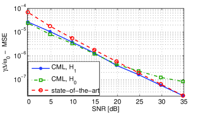
(a) $\Delta=0.1\times 2\pi$

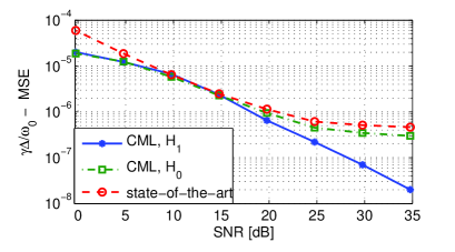
(b) $\Delta=2.5\times 2\pi$

Figure 1: The MSE of the normalized frequency deviation, $\gamma\frac{\Delta}{\omega_{0}}$, estimators for $K=12$, $N=48$, and for (a) $\Delta=0.1\times 2\pi$; and (b) $\Delta=2.5\times 2\pi$.

V-B Single-phase magnitude and phase imbalances

The performance of the proposed GLRT is compared with the performance of the commonly-used VUF method for detecting voltage imbalance [4], [16], [17]. The VUF test is defined as the ratio of the negative-sequence voltage magnitude to the positive-sequence voltage magnitude. In order to make a fair comparison, we use the VUF definition with $K$ phasor measurements of the positive- and negative-sequence:

$$T_{\text{VUF}}=\frac{\frac{1}{K}\sum_{k=0}^{K-1}\left|V_{-}[k]\right|}{\frac{1}{K}\sum_{k=0}^{K-1}\left|V_{+}[k]\right|},$$ (78)

which is based only on the voltage magnitudes. It should be noted that there is no analytical procedure for setting the threshold of the VUF detector, $T_{\text{VUF}}$. In the following, we chose the threshold to maximize the probability of detection for each scenario.

In addition, in order to demonstrate power loss due to the unknown frequency deviation, i.e. reduction in detection probability for a given probability of error ratio, we also compare the results with a GLRT for known frequency deviation, $\Delta$. This detector is given by the GLRT in (66), in which we substitute the known frequency deviation in $P$, $Q$, ${\bf{e}}_{1}$, and ${\bf{e}}_{2}$, which affects the ML phasor estimators and $\kappa_{1},\kappa_{2}$. When the estimation error is small, the known frequency-deviation GLRT is expected to be close to the proposed GLRT.

In this case, single-phase voltage magnitude and phase imbalance is considered by changing the voltage magnitude and phase of the single-phase $c$, i.e. by changing $\beta$ and $\epsilon$. In Figs. 2.a and 2.b, the probability of detection is presented versus different values of $\beta$ and $\epsilon$, respectively, for a constant false alarm probability of $15\%$. When $\beta$ approaches $1.03$ or $\epsilon$ approaches $\frac{3}{100}\pi$, a reduction occurs in the detection probability since the magnitude or phase voltage imbalance is smaller and identical to the balanced scenario. In this case, the probability of detection is equal to the probability of error, i.e. equal to $0.15$. It can be seen that the detection probability of the GLRT is significantly higher than that of the VUF for any scenario. In addition, for high SNR the performance of the GLRT with estimated frequency deviation coincides with the known-frequency GLRT. It can be seen that the GLRT and VUF are robust to this scenario outside the local region of small insignificant imbalances and these detectors are able to distinguish between true imbalances (higher than $3\%$) and low unbalances. The GLRT detection probability is higher than that of the VUF in this case too. Fig. 2.b examines that the proposed methods are symmetric w.r.t. clockwise and anticlockwise movement of phasor $c$.

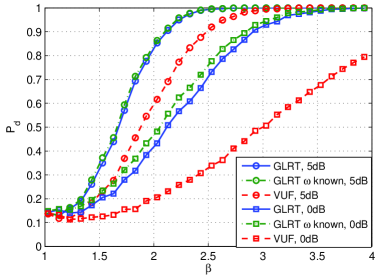
(a) Magnitude imbalance

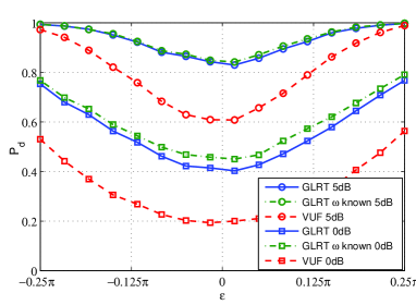
(b) Phase imbalance

Figure 2: Magnitude and phase imbalances: The probability of detection of VUF and GLRT with known/unknown frequency deviation for a constant probability of false alarm of $15\%$ and $K=12$, $N=48$, $\Delta=0.1\times 2\pi$, $V_{a}=1$, $\varphi_{a}=0.25\pi$ and SNR$=0,5$ dB are presented: (a) versus $\beta$ for $\epsilon=0$; and (b) versus $\epsilon$ for $\beta=2$.

In order to examine the influence of the number of samples at the frequency domain, $K$, on the detection performance, the probability of detection is presented versus $K$ in 3 for a constant false alarm probability of $15\%$ and SNR$=0,5$ dB. It can be seen that for a large number of frequency domain samples, $K$, the effect of frequency deviation is reduced. In particular, for $K>15$, the performance of the GLRT with estimated frequency deviation is very close to the performance of the known-frequency GLRT for both SNR. In contrast to the GLRTs, for low SNR an increase in $K$ does not improve the performance since the VUF is not robust to the local-imbalances scenario. For high SNR, the probability of detection of the VUF increases with $K$ but it is lower than the probability of detection of the two GLRTs.

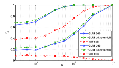
Figure 3: The probability of detection of VUF and GLRT with known/unknown frequency deviation versus $K$ for a constant probability of false alarm of $15\%$ and $\epsilon=0$, $\beta=2$, $N=24$, $\Delta=0.1\times 2\pi$, $V_{a}=1$, $\varphi_{a}=0.25\pi$ and SNR$=0,5$ dB.

V-C Case study: Imbalance detection in the presence of higher order harmonics

Usually, there are additional harmonics where the harmonics frequencies are multiples of the prevailing off-nominal network frequency [1]. The performance of the GLRT is influenced by the imbalance degree and the voltage signal harmonic distortion. In order to model the influence of the harmonics, we replace the model in (7) by (e.g. [1]):

$$\left[\begin{array}[]{c}v_{a}[n]\\ v_{b}[n]\\ v_{c}[n]\end{array}\right]=\left[\begin{array}[]{c}V_{a}\sum_{p=1}^{P}a_{p}\cos\left(p(\gamma\frac{\omega_{0}+\Delta}{\omega_{0}}n+\varphi_{a})\right)\\ V_{b}\sum_{p=1}^{P}a_{p}\cos\left(p(\gamma\frac{\omega_{0}+\Delta}{\omega_{0}}n+\varphi_{b})\right)\\ V_{c}\sum_{p=1}^{P}a_{p}\cos\left(p(\gamma\frac{\omega_{0}+\Delta}{\omega_{0}}n+\varphi_{c})\right)\end{array}\right]$$ (85)

$$+{\bf{w}}_{a,b,c}[n],\hskip 128.0374pt$$

where we set $P=4$, $a_{1}=1$, $a_{2}=0.2$, $a_{3}=0$, and $a_{4}=0.5$. The other parameters are chosen to be the same parameters as in Subsection V-B. The detectors’ performance is presented for the case of non-sinusoidal and voltage imbalance in Fig. 4. By comparing the probabilities of detection in 4 and 2 it can be seen that the performance degradation is not significant and the proposed GLRT methods, as well as the existing VUF method, is not sensitive to inter-harmonics. Therefore, the proposed methods for detection of unbalances can be used also in the presence of harmonics.

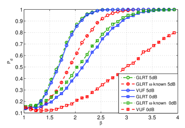
(a) Magnitude imbalance

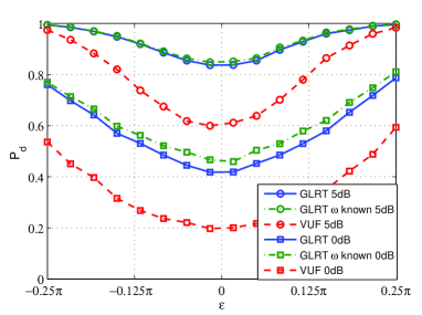
(b) Phase imbalance

Figure 4: Magnitude and phase imbalances for non-sinusoidal signals: The probability of detection of VUF and GLRT with known/unknown frequency deviation for a constant probability of false alarm of $15\%$ and $K=12$, $N=48$, $\Delta=0.1\times 2\pi$, $V_{a}=1$, $\varphi_{a}=0.25\pi$ and SNR$=0,5$ dB and with two additional harmonics are presented: (a) versus $\beta$ for $\epsilon=0$; and (b) versus $\epsilon$ for $\beta=2$.

V-D Probability of error

The simulated false alarm probability of the GLRT and GLRT-SNH with known/unknown frequency deviation and the theoretical probability of error from (76) are presented in Fig. 5 versus the threshold, $\tau$, for an unbalanced system with $\beta=2$, $\epsilon=0.1\pi$, $K=12$ frequency samples, and for an SNR of $10$ dB. According to (76), the probability of error is a function of the threshold $\tau$ and $r$, but is independent of the noise level. Therefore, Fig. 5 represents the results for any SNR. It can be seen that the theoretical false alarm probability captures the behavior of the actual false alarm probability of the GLRT and GLRT-SNH even in the unknown-frequency case. That is, the theoretical asymptotic performance (or equivalently, the performance in the known frequency-deviation case) adequately summarizes the actual performance for data records as short as $K=12$ samples. Thus, we can conclude that although the asymptotic bound theoretically requires an infinite number of observations, it still provides a tight lower bound on the probability of error when there is a sufficiently large observation window for both GLRT and GLRT-SNH. In addition, it can be verified that for the same threshold value, the GLRT-SNH has higher probability of error.

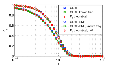
Figure 5: The asymptotic and simulated probability of error of the GLRT and GLRT-SNH with known/unknown frequency deviation for $K=12$, $N=48$, $\Delta=0.1\times 2\pi$, $V_{a}=1$, $\varphi_{a}=0.25\pi$, $\beta=1.75$, $\epsilon=0.1\pi$, and SNR$=0$ dB.

VI Conclusion

In this study we demonstrate the detection of imbalances by using the PMU output of the symmetrical components when the voltage measurements are noise contaminated. We formulate the detection of imbalance as a hypothesis testing problem with unknown constrained parameters within the framework of detection theory. The GLRT is derived for this problem and the CML phasors’ estimators are developed for both balanced and unbalanced systems and can be used for general state-estimation in a smart grid. The known-frequency and asymptotic performance of the proposed GLRT detector has been provided and can be used as a benchmark. In detection theory, different tests induce different thresholds that the likelihood ratio is compared to [38]. Thus, the threshold setting is the key component of the hypothesis testing. In this context, a new formulation is devised for setting the threshold that also interpolates the authorized level of imbalances.

Simulation results have verified that the proposed GLRT with either known or estimated frequency deviation yields competitive performance, compared to the state-of-the-art VUF method and is better for magnitude imbalance detection. In addition, we demonstrate that the proposed method is not sensitive to additional harmonics. Topics for future research include the derivation of mitigation techniques that use the proposed GLRT as an imbalance measure in order to correct unbalanced voltage problems more efficiently. In addition, real-time implementation of the proposed detectors can be very important, especially the derivation of a change detection method for imbalances.

References

- [1] A. Phadke and J. Thorp, Synchronized Phasor Measurements and Their Applications. New York: Springer Science, 2008.
- [2] “Electric power systems and equipment voltage ratings (60 Hertz),” ANSI Standard Publication, no. ANSI C84.1, 1995.
- [3] S. Zhong and A. Abur, “Effects of nontransposed lines and unbalanced loads on state estimation,” in IEEE Power Engineering Society Winter Meeting, vol. 2, Jan. 2002, pp. 975–979.
- [4] A. Von Jouanne and B. Banerjee, “Assessment of voltage unbalance,” IEEE Trans. Power Delivery, vol. 16, no. 4, pp. 782–790, Oct. 2001.
- [5] N. D. Tleis, Power Systems Modelling and Fault Analysis: Theory and Practice. Oxford : Newnes, 2008.
- [6] N. Woolley and J. Milanovic, “Statistical estimation of the source and level of voltage unbalance in distribution networks,” IEEE Trans. Power Delivery, vol. 27, no. 3, pp. 1450–1460, July 2012.
- [7] M. T. Bina and A. Kashefi, “Three-phase unbalance of distribution systems: Complementary analysis and experimental case study,” International Journal of Electrical Power & Energy Systems, vol. 33, no. 4, pp. 817–826, 2011.
- [8] T. H. Chen, C. H. Yang, and N. C. Yang, “Examination of the definitions of voltage unbalance,” International Journal of Electrical Power & Energy Systems, vol. 49, pp. 380–385, 2013.
- [9] A. Gomez-Exposito, A. Abur, A. de la Villa Jaen, and C. Gomez-Quiles, “A multilevel state estimation paradigm for smart grids,” Proceedings of the IEEE, vol. 99, no. 6, pp. 952–976, June 2011.
- [10] A. G. Phadke, J. S. Thorp, and M. G. Adamiak, “A new measurement technique for tracking voltage phasors, local system frequency, and rate of change of frequency,” IEEE Trans. Power Apparatus and Systems, vol. PAS-102, no. 5, pp. 1025–1038, May 1983.
- [11] Y. Xia, S. Douglas, and D. Mandic, “Adaptive frequency estimation in smart grid applications: Exploiting noncircularity and widely linear adaptive estimators,” IEEE Signal Processing Magazine, vol. 29, no. 5, pp. 44–54, Sep. 2012.
- [12] Y. Xia and D. Mandic, “Widely linear adaptive frequency estimation of unbalanced three-phase power systems,” IEEE Trans. Instrumentation and Measurement, vol. 61, no. 1, pp. 74–83, Jan. 2012.
- [13] P. Yang, Z. Tan, A. Wiesel, and A. Nehorai, “Power system state estimation using PMUs with imperfect synchronization,” IEEE Trans. Power Systems, vol. 28, no. 4, pp. 4162–4172, Nov. 2013.
- [14] A. Angioni, C. Muscas, S. Sulis, F. Ponci, and A. Monti, “Impact of heterogeneous measurements in the state estimation of unbalanced distribution networks,” in Instrumentation and Measurement Technology Conference (I2MTC), 2013 IEEE International, May 2013, pp. 935–939.
- [15] B. Van Tuykom, J. C. Maun, and A. Abur, “Use of phasor measurements and tuned weights for unbalanced system state estimation,” in North American Power Symposium (NAPS), 2010, Sep. 2010, pp. 1–5.
- [16] P. Pillary and M. Manyage, “Definitions of voltage unbalance,” IEEE Power Eng. Rev., vol. 21, no. 5, pp. 49–51, May 2001.
- [17] M. H. J. Bollen, “Definitions of voltage unbalance,” IEEE Power Eng. Rev., vol. 22, no. 11, pp. 49–50, Nov. 2002.
- [18] A. Singh, G. Singh, and R. Mitra, “Some observations on definitions of voltage unbalance,” in Power Symposium, 2007. NAPS ’07. 39th North American, 2007, pp. 473–479.
- [19] C. Y. Lee, “Effects of unbalanced voltage on the operation performance of a three-phase induction motor,” IEEE Trans. Energy Conversion, vol. 14, no. 2, pp. 202–208, June 1999.
- [20] J.-G. Kim, E.-W. Lee, D.-J. Lee, and J.-H. Lee, “Comparison of voltage unbalance factor by line and phase voltage,” in Electrical Machines and Systems, 2005. ICEMS 2005. Proceedings of the Eighth International Conference on, vol. 3, Sep. 2005, pp. 1998–2001 Vol. 3.
- [21] P. Pillay and P. Hofmann, “Derating of induction motors operating with a combination of unbalanced voltages and over- or undervoltages,” in IEEE Power Engineering Society Winter Meeting, 2001., vol. 3, 2001, pp. 1365–1371.
- [22] J. Faiz, H. Ebrahimpour, and P. Pillay, “Influence of unbalanced voltage on the steady-state performance of a three-phase squirrel-cage induction motor,” IEEE Trans. Energy Conversion, vol. 19, no. 4, pp. 657–662, Dec. 2004.
- [23] A. Ferreira Filho, J. Cormane, D. Garcia, M. V. C. Costa, M. A. G. Oliveira, and F. do Nascimento, “Analysis of the complex voltage unbalance factor behavior resulting from the variation of voltage magnitudes and angles,” in International Conference on Harmonics and Quality of Power (ICHQP), Sep. 2010, pp. 1–7.
- [24] J. Faiz and H. Ebrahimpour, “Precise derating of three-phase induction motors with unbalanced voltages,” in Industry Applications Conference, IAS Annual Meeting, vol. 1, Oct. 2005, pp. 485–491.
- [25] M. Sun, S. Demirtas, and Z. Sahinoglu, “Joint voltage and phase unbalance detector for three phase power systems,” IEEE Signal Processing Letters, vol. 20, no. 1, pp. 11–14, Jan. 2013.
- [26] J. Arrillaga, M. H. J. Bollen, and N. Watson, “Power quality following deregulation,” Proceedings of the IEEE, vol. 88, no. 2, pp. 246–261, Feb. 2000.
- [27] D. Santos-Martin, J. Rodriguez-Amenedo, and S. Arnalte, “Direct power control applied to doubly fed induction generator under unbalanced grid voltage conditions,” IEEE Trans. Power Electronics, vol. 23, no. 5, pp. 2328–2336, Sep. 2008.
- [28] M. Davoudi, A. Bashian, and J. Ebadi, “Effects of unsymmetrical power transmission system on the voltage balance and power flow capacity of the lines,” in International Conference on Environment and Electrical Engineering (EEEIC), May 2012, pp. 860–863.
- [29] A. Ghosh and A. Joshi, “A new approach to load balancing and power factor correction in power distribution system,” IEEE Trans. Power Delivery, vol. 15, no. 1, pp. 417–422, Jan. 2000.
- [30] M. Savaghebi, A. Jalilian, J. Vasquez, and J. Guerrero, “Autonomous voltage unbalance compensation in an islanded droop-controlled microgrid,” IEEE Trans. Industrial Electronics, vol. 60, no. 4, pp. 1390–1402, Apr. 2013.
- [31] A. Bidram and A. Davoudi, “Hierarchical structure of microgrids control system,” IEEE Trans. Smart Grid, vol. 3, no. 4, pp. 1963–1976, Dec. 2012.
- [32] A. Elnady and M. Salama, “Mitigation of voltage disturbances using adaptive perceptron-based control algorithm,” IEEE Trans. on Power Delivery, vol. 20, no. 1, pp. 309–318, Jan. 2005.
- [33] B. Meersman, B. Renders, L. Degroote, T. Vandoorn, and L. Vandevelde, “Three-phase inverter-connected DG-units and voltage unbalance,” Electric Power Systems Research, vol. 81, no. 4, pp. 899–906, 2011.
- [34] T. Routtenberg and L. Tong, “Joint frequency and phasor estimation in unbalanced three-phase power systems,” in ICASSP 2014, May 2014, pp. 3006–3010.
- [35] D. Fan and V. Centeno, “Phasor-based synchronized frequency measurement in power systems,” IEEE Trans. Power Delivery, vol. 22, no. 4, pp. 2010–2016, 2007.
- [36] J. Li, X. Xie, J. Xiao, and J. Wu, “The framework and algorithm of a new phasor measurement unit,” in IEEE International Conference on Electric Utility Deregulation, Restructuring and Power Technologies (DRPT), vol. 2, Apr. 2004, pp. 826–831.
- [37] Y. Wang, “Modeling of random variation of three-phase voltage unbalance in electric distribution systems using the trivariate gaussian distribution,” Generation, Transmission and Distribution, IEE Proceedings-, vol. 148, no. 4, pp. 279–284, July 2001.
- [38] S. M. Kay, Fundamentals of Statistical Signal Processing: Detection Theory. Englewood Cliffs (N.J.): Prentice Hall PTR, 1998, vol. 2.
- [39] T. Moore and B. Sadler, “Constrained hypothesis testing and the Cramr-Rao bound,” in Proc. Sensor Array and Multichannel Signal Processing Workshop (SAM) 2010, Oct. 2010, pp. 113–116.
- [40] S. Boyd and L. Vandenberghe, Convex Optimization. New York, NY, USA: Cambridge University Press, 2004.
- [41] V. Terzija, N. Djuric, and B. Kovacevic, “Voltage phasor and local system frequency estimation using Newton type algorithm,” IEEE Trans. Power Delivery, vol. 9, no. 3, pp. 1368–1374, July 1994.
- [42] P. Top, M. Bell, E. Coyle, and O. Wasynczuk, “Observing the power grid: Working toward a more intelligent, efficient, and reliable smart grid with increasing user visibility,” IEEE Signal Processing Magazine, vol. 29, no. 5, pp. 24–32, 2012.