Fisher-Shannon product and quantum revivals in wavepacket dynamics

Abstract

We show the usefulness of the Fisher-Shannon information product in the study of the sequence of collapses and revivals that take place along the time evolution of quantum wavepackets. This fact is illustrated in two models, the quantum bouncer and a graphene quantum ring.

1 Introduction

Sequences of collapses and revivals in the wavepackets temporal evolution are a well known aspect of quantum dynamics. This phenomenon has been theoretically understood [1] and to date it has been observed in striking experiments with atoms and molecules [2, 3], Bose-Einstein condensates [4, 5] and recently in coherent states in a Kerr medium [6]. Moreover, quantum revivals have been studied theoretically in low-dimensional quantum structures as graphene, graphene quantum dots and rings in perpendicular magnetic fields [7, 8, 9, 10, 11, 12, 13, 14, 15]

In this paper we show that the analysis of wavepacket quantum revivals can be carried out using the Fisher-Shannon product $P_{\rho}$, defined as [16]:

$$P_{\rho}=I_{\rho}N_{\rho}$$ (1)

with

$$I_{\rho}=\int\frac{|\nabla\rho(x)|^{2}}{\rho(x)}dx$$ (2)

being the Fisher information,

$$S_{\rho}=-\int\rho(x)\ln\rho(x)dx$$ (3)

the Shannon entropy, and $N_{\rho}=\exp{(2S_{\rho}})/(2\pi e)$ the so-called entropy power [17]. It is known that these information measures show complementary descriptions of the spreading or concentration of the probability density, where the Fisher information gives a local measure of the spreading (due to the gradient in the functional form), whereas the Shannon entropy provides a global one. This entropic product has proved useful in the analysis of different physical situations, i. e., electronic correlation [16], atomic physics [18, 19, 20], chemical reactions [21], quantum phase transitions [22], astrophysics [23] or in the study of geophysical phenomena [24]. There is a generalization of the Fisher-Shannon product, the so-called Fisher-Rényi product [25]. Note here the existence of other important complexity measures which have also been used in the description of a great variety of systems (see [26] and references therein).

We shall consider the Fisher-Shannon information product as it applies to quantum revival phenomena. In particular, we shall show the role of this quantity in the dynamics of two model systems that exhibits sequences of quantum collapses and revivals: the so-called quantum ‘bouncer’ (that is a quantum particle bouncing against a hard surface under the influence of gravity) and a graphene quantum ring model.

2 Wave packet dynamic and Fisher-Shannon product

It is well known that the temporal evolution of localized bound states $\psi$ for a time independent Hamiltonian is given in terms of the eigenvectors $u_{n}$ and eigenvalues $E_{n}$ as

$$\psi(t)=\sum_{n=0}c_{n}u_{n}e^{-iE_{n}t/\hbar},$$ (4)

where $c_{n}=\langle u_{n},\psi\rangle$ are the Fourier components of the vector $\psi$, and $n$ is the main quantum number of the system (in general one has to consider the set of quantum numbers corresponding to the system, see [1], but in this paper we will consider only systems with one quantum number). Now, a wavepacket is constructed with the coefficients $c_{n}$ tightly centered around a large value of $n_{0}\gg|n-n_{0}|$, with $n_{0}\gg 1$. The exponential factor in (4) can then be written as a Taylor expansion around $n_{0}$ (within this approximation, $n$ is a continuous variable) as

$$\exp\left(-iE_{n}t/\hbar\right) =\exp\left[-i(E_{n_{0}}+E_{n_{0}}^{\prime}(n-n_{0})+E_{n_{0}}^{\prime\prime}/2(n-n_{0})^{2}+\cdots)t/\hbar\right]$$

$$= \exp\left(-i\omega_{0}t-2\pi i(n-n_{0})t/T_{\rm Cl}-2\pi i(n-n_{0})^{2}t/T_{\rm R}+\cdots\right)$$ (5)

where each term in the exponential (except for the first one, which is a global phase) defines a characteristic time scale, that is, $T_{\rm R}\equiv\frac{4\pi\hbar}{|E_{n_{0}}^{\prime\prime}|}$ and $T_{\rm Cl}\equiv\frac{2\pi\hbar}{|E_{n_{0}}^{\prime}|}$ (see [1] for more details). The so called fractional revival times can be given in terms of the quantum revival time-scale by $t=pT_{\rm R}/q$, where $p$ and $q$ are mutually prime.

Next, we study the wave packet dynamics by means of the so-called entropy product, i.e., the product of the Fisher information and the Shannon entropy power, $N_{\rho}$, to conclude that it provides another framework for visualizing fractional revival phenomena. Again, we expect that the formation of a number of minipackets of the original packet will correspond to relative minima of the information product. Before proceeding, recall that $P_{\rho}$ satisfies the isoperimetric inequality [17]

$$P_{\rho}=I_{\rho}N_{\rho}\geq 1.$$ (6)

The equality is reached for Gaussian densities. By combining the above inequality with the Stam uncertainty principle [27]

$$I_{\rho}\geq\frac{4}{\hbar^{2}}(\Delta p)^{2},$$ (7)

and the power entropy inequality [28]

$$N_{\rho}\leq(\Delta x)^{2},$$ (8)

leads to the usual formulation of the uncertainty principle in terms of the variance in conjugate spaces, $\Delta p\Delta x\geq\hbar/2$. It is straightforward to show that the equality limit of these four inequalities is reached for Gaussian densities.

2.1 Quantum bouncer

Quantum states of matter in a gravitational field have been recently realized experimentally with neutrons [29, 30]. These were allowed to fall towards a horizontal mirror which, together with the Earth’s gravitational field, provided the necessary confining potential well. From a theoretical point of view, this constitutes an example of the quantum variant of a classical particle subject to a uniform downward force, above an impermeable flat surface. The revival behavior of quantum bouncers has been discussed in [31, 32] and an entropy-based approach was carried out in [33, 34]. Here, we shall evaluate the goodness of the entropy-product when applied to a quantum bouncer.

The time dependent solution of the Schrödinger equation for the potential $V(z)=mgz$ if $z\geq 0$ and $V(z)=0$ otherwise reads

$$\Psi(z,t)=\sum_{n=1}^{\infty}c_{n}e^{-iE_{n}t/\hbar}\varphi_{n}(z),$$ (9)

where the eigenfunctions and eigenvalues are given by [32]

$$E^{\prime}_{n}=z_{n};\quad\varphi_{n}(z^{\prime})={\mathcal{N}}_{n}{\rm Ai}(z^{\prime}-z_{n});\quad n=1,2,3,\ldots.$$ (10)

In the above equation, position and energy variables have been rescaled, $z^{\prime}=z/l_{g}$, $E^{\prime}=E/mgl_{g}$, and are denoted by primed symbols. $l_{g}=\left(\hbar/2gm^{2}\right)^{1/3}$ is a characteristic gravitational length, ${\rm Ai}(z)$ is the Airy function, $-z_{n}$ denotes its zeros, and ${\mathcal{N}}_{n}$ is the $\varphi_{n}(z^{\prime})$ normalization factor. $z_{n}$ and ${\mathcal{N}}_{n}$ were determined numerically by using scientific subroutine libraries for the Airy function, although accurate analytic approximations for them can be found in [32]. In the remainder of this paper, the primes on the energy and position variables will be omitted and we shall assume initial conditions that correspond to Gaussian wave packets localized at a height $z_{0}$ above the surface, with a width $\sigma$ and an initial momentum $p_{0}=0$,

$$\Psi(z,0)=\left(\frac{2}{\pi\sigma^{2}}\right)^{1/4}e^{-(z-z_{0})^{2}/\sigma^{2}}.$$ (11)

The corresponding coefficients $c_{n}$ of the wave function (9) can be obtained analytically as [35],

$$c_{n}= {\mathcal{N}}_{n}\left(2\pi\sigma^{2}\right)^{1/4}\exp\left[\frac{\sigma^{2}}{4}\left(z_{0}-z_{n}+\frac{\sigma^{4}}{24}\right)\right]$$ (12)

$$\times{\rm Ai}\left(z_{0}-z_{n}+\frac{\sigma^{4}}{16}\right),$$

with ${\mathcal{N}}_{n}=|{\rm Ai}^{\prime}(-z_{n})|$. It is now a straightforward calculation to obtain for the classical period and the revival time $T_{\rm Cl}=2\sqrt{z_{0}}$ and $T_{\rm R}=4z_{0}^{2}/\pi$, respectively [32]. The temporal evolution of the wave packet in momentum-space is obtained numerically by the fast Fourier transform method.

We have computed the temporal evolution of the entropy product (1) for the initial conditions $z_{0}=100$, $p_{0}=0$, and $\sigma=1$. Figure 1 displays $P_{\rho}$ and the location of the main fractional revivals. It can be neatly observed that the entropic product decreases and reaches a minimum at most of the fractional revivals, where the quasiclassical behavior and a Gaussian shape are recovered.

Notice how the initial value of unity for the information product is approximately recovered at the full revival, when the Gaussian form of the wavepacket is roughly restored.

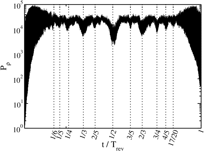
Figure 1: Time dependence of the Fisher-Shannon product for an initial Gaussian wave packet with $z_{0}=100,p_{0}=0$, and $\sigma=1$ in a quantum bouncer. The main fractional revivals are indicated by vertical dotted lines.

2.2 Graphene quantum ring

We shall consider the behavior of the Fisher-Shannon information in another physical situation. Let us consider a graphene quantum ring within a simplified model [36, 37, 38, 39] which is described by the Hamiltonian

$$H=v_{F}\vec{p}\hskip 1.42271pt\vec{\sigma}+\tau\Delta\sigma_{z},$$ (13)

where $\tau=\pm 1$ corresponds to each of the two inequivalent corners $K$ and $K^{\prime}$ of the first Brillouin zone, $\vec{p}$ is the momentum measured relatively to the $K$ ($K^{\prime}$) point, $\Delta$ a finite mass term, $v_{F}\simeq 10^{6}$ m/s is the Fermi velocity, and $\vec{\sigma}=(\sigma_{x},\sigma_{y},\sigma_{z})$ where the components are the Pauli matrices. We shall work using a geometrical approximation of a zero width ring with radius $R$ (used in [36, 37, 38, 39]). The eigenstates and eigenfunctions are given in polar coordinates by [36]

$$\Phi_{m}(R,\phi)=\left(\begin{array}[]{cc}\phi_{A}(R)e^{im\phi}\\ i\phi_{B}(R)e^{i(m+1)\phi}\\ \end{array}\right),$$ (14)

$$\phi_{A}(R)=1,\quad\quad\phi_{B}(R)=\frac{m+\frac{1}{2}}{\epsilon+\tau\nu},$$ (15)

$$\epsilon=\pm\sqrt{(m+1)m+\nu^{2}+1/4},$$ (16)

where $E_{0}\equiv\hbar v_{F}/R$, $\nu\equiv\Delta/E_{0}$ and $\epsilon\equiv E/E_{0}$, and with $\hbar(m+1/2)$ with $m=-j$, $-j+1$, $\ldots j$ being the eigenvalue of the total angular momentum $J_{z}=L_{z}+\hbar S_{z}$.

Now we shall construct the initial wave packet centered around an eigenvalue $E_{m_{0}}$. In Fig. 2 the Fisher-Shannon product for a ring of $R=50$ nm, $\Delta=50$ meV and $E_{m_{0}}\approx 200$ meV is depicted. We can observe a quasiclassical evolution (with a period of $T_{\rm R}=0.078$ ns) at early times, which corresponds to a minimum in the Fisher-Shannon product. We can see that at $T_{\rm R}/2$ (and at multiples times of it), where the wave-packet recovers its quasiclassical behavior, we have a relative minimum again.

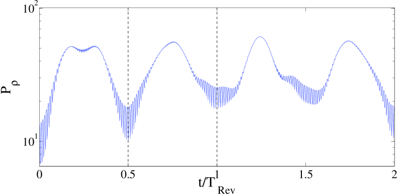
Figure 2: Time dependence of the entropic product for an initial Gaussian wavepacket with $E_{m_{0}}\approx 200$ meV, $\sigma=13$, for a quantum ring with $R=50$ nm, $\Delta=50$ meV.

3 Summary

We have presented an analysis of quantum wavepacket revival phenomena in the quantum bouncer and a graphene ring, based on the information product. We have shown that this theoretical tool (which has proved to be useful for the analysis of different phenomena in atomic physics, molecular reactions, solids, and even in geophysics) appropriately describes the dynamics of wavepackets. In particular, we have found that the revivals and fractional revivals of wavepackets correspond to relative minima in the entropic product, signaling the recovery of the quasiclassical behavior of the wavepacket.

4 Acknowledgments

This work was supported by the Spanish Projects No. MICINN FIS2009-08451, No. FQM-02725 (Junta de Andalucía), and No. MICINN FIS2011-24149.

References

- [1] R. W. Robinett, Phys. Rep. 392 1, (2004).
- [2] G. Rempe, H. Walther, and N. Klein, Phys. Rev. Lett. 58, 353 (1987); J. A. Yeazell, M. Mallalieu, and C. R. Stroud, Jr., Phys. Rev. Lett. 64, 2007 (1990); T. Baumert et al., Chem. Phys. Lett. 191, 639 (1992); M.J.J. Vrakking, D. M. Villeneuve, and A. Stolow, Phys. Rev. A 54, R37-R40 (1996); A. Rudenko et al T. Ergler, and B. Feuerstein et al., Chem. Phys. 329, 193 (2006).
- [3] S. Will, T. Best, U. Schneider, L. Hackermüller, D. Lühmann and I. Bloch, Nature 465, 197 (2010)
- [4] M. Greiner, M. O. Mandel, T. Hänsch, and I. Bolch, Naure 419, 51 (2002).
- [5] J. Sebby-Strabley et al. Phys. Rev. Lett. 98, 200405 (2007).
- [6] G. Kirchmair, B. Vlastakis, Z. Leghtas, S. E. Nigg, H. Paik, E. Ginossar, M. Mirrahimi, L: Frunzio, S. M. Girvin and R. J. Schoelkopf, Nature 495, 205 (2013).
- [7] E. Romera and F. de los Santos, Phys. Rev. B 80, 165416 (2009).
- [8] V. Krueckl and T. Kramer, New J. Phys. 11, 093010 (2009).
- [9] A. Chaves, L. Covaci, Kh. Yu. Rakhimov, G. A. Farias, and F. M. Peeters, Phys. Rev. B 82, 205430 (2010).
- [10] J. Luo, D. Valencia, and J. Lu, J. of Chem. Phys. 135, 224707 (2011).
- [11] Y. Wang, Y. He and S. Xiong, Mod. Phys. Lett. 26, 1250139 (2012).
- [12] A. López, Z. Z. Sun, and J. Schliemann, Phys. Rev. B, 85 205428 (2012).
- [13] Tomasz M. Rusin and Wlodek Zawadzki, Phys. Rev. B, 78, 215419 (2008).
- [14] John Schliemann, New J. Phys. 10, 043024 (2008).
- [15] V. Ya. Demikhovskii, G. M. Maksimova, A. A. Perov and A. V. Telezhnikov, Phys. Rev. A, 85, 022105 (2012).
- [16] E. Romera, and J. S. Dehesa, J. Chem. Phys. 120, 8906 (2004).
- [17] See A. Dembo, T.M. Cover, and J.A. Thomas, IEEE Trans. Inf. Theory 37, 1501 (1991), and references therein.
- [18] Á. Nagy and E. Romera I. J. Quan. Chem. 109 2490 (2009).
- [19] J. Sañudo and R. López-Ruiz, Phys. Lett. A 372, 2549 (2009).
- [20] S. Liu J. Chem. Phys. 126, 191107 (2007).
- [21] R. O. Esquivel et al. Theo. Chem. Acc. 124, 445 (2009).
- [22] Á. Nagy, E. Romera Physica A 391 3650 (2012).
- [23] M. Lovallo et al. J. Stat. Mech. 2011, P03029 (2011)
- [24] L. Telesca, M. Lovallo, A. Chamoli, V. P. Dimri, K. Srivastava Physica A, 392, 3424 (2013).
- [25] E. Romera, and Á. Nagy, Phys. Lett. A 372, 6823 (2008).
- [26] R. López-Ruiz et al. J. Math. Phys. 50, 123528 (2009).
- [27] A.J. Stam, Information and Control 2, 101 (1959).
- [28] I. Bialynicki-Birula and J. Mycielski, Comm. Math. Phys. 44, 129 (1975); W. Beckner, Ann. Math. 102, 159 (1975).
- [29] Valery V. Nesvizhevsky et al Nature 415, 297-299 (2002); V.V. Nesvizhevsky, A.K. Petukhov, K.V. Protasov, and A.Yu. Voronin, Phys. Rev. A 78, 033616 (͑2008).
- [30] V.V. Nesvizhevsky and K.V. Protasov, Quantum states of neutrons in the Earth’s gravitational field: state of the art , applications, perspectives, in Trends in Quantum Gravity Research Editor David C. Moore, pp. 65-107 Nova Science Publishers, Inc. (2006).
- [31] M.A. Doncheski and R. W. Robinett, Am. J. Phys. 69 2001
- [32] J. Gea-Banacloche, Am. J. Phys. 67, 776 (1999).
- [33] E. Romera and F. de los Santos, Phys. Rev. Lett. 99, 263601 (2007).
- [34] E. Romera and F. de los Santos, Phys. Rev. A 78, 013837 (2008).
- [35] O. Vallée , Am. J. Phys. 68, 672 (2000).
- [36] M. Zarenia, J. Milton Pereira, A. Chaves, F. M. Peeters, and G. A. Farias, Phys. Rev. B 81, 045431 (2010); Phys. Rev. B 81, 045431(E) (2010).
- [37] F. E. Meijer, A. F. Morpurgo and T. M. Klapwijk, Phys. Rev. B 66, 033107 (2002).
- [38] B. Molnár, F. M. Peeters, and P. Vasilopoulos, Phys. Rev. B 69, 155335 (2004).
- [39] T. García, S. Rodríguez-Bolivar, N. Cordero and E. Romera, J. Phys: Condens. Matter 25, 235301 (2013).