Resonances in the
Two-Centers Coulomb Systems

Abstract

We investigate the existence of resonances for two-centers Coulomb systems with arbitrary charges in two dimensions, defining them in terms of generalised complex eigenvalues of a non-selfadjoint deformation of the two-centers Schrödinger operator. We construct the resolvent kernels of the operators and prove that they can be extended analytically to the second Riemann sheet. The resonances are then analysed by means of perturbation theory and numerical methods.

Mathematics Subject Classification: 34E20, 34F15, 35P15, 81U05, 81V55

1 Introduction

Our work concerns the study of the quantum mechanical two-fixed-centers Coulomb systems in two dimensions. The two-dimensional restriction of the two-centers problem arises naturally in the analysis of the three-dimensional problem and, as described in [48], it is essential to be able to analyse that case.

Since three centuries the two-centers Coulombic systems have been studied, from a classical and later also from a quantum mechanical point of view, starting from pioneering works of Euler, Jacobi [28] and Pauli [43] and going on until the recent years. For an historical overview we refer the reader to [48].

The interest for the quantum mechanical version of the problem comes mainly from molecular physics. Indeed it defines the simplest model for one-electron diatomic molecules (e.g. the ions ${\rm H}_{2}^{+}$ and ${\rm He}\,{\rm H}^{++}$) and a first approximation of diatomic molecules in the Born-Oppenheimer representation.

In fact many of the results in the literature are related to the hard problem of finding algorithms to obtain good numerical approximations of the discrete spectrum and of the scattering waves [22, 23, 35, 36, 47], and to the asymptotic analysis of spectral properties in the very small or very large center distance [10, 15, 21, 31]. In contrast, really little is known on the regularity of the solutions with respect to the parameters of the system [52] and even less on the problem of resonances.

Quantum resonances are a key notion of quantum physics: roughly speaking these are scattering states (i.e. states of the essential spectrum) that for long time behave like bound states (i.e. eigenfunctions). They are usually defined as poles of a meromorphic function, but note that there is no consensus on their definition and their study [62]. On the other hand, it is known that many of their definitions coincide in some settings [26] and that their existence is related to the presence of some classical orbits “trapped” by the potential.

If a quantum systems has a potential presenting a positive local minimum above its upper limit at infinity, for example, it is usually possible to find quantum resonances, called shape resonances. These are related to the classical bounded trajectories around the local minimum [27]. These are not the only possible ones: it has been proven in [7, 8, 20, 50] that there can be resonances generated by closed hyperbolic trajectories or by a non-degenerate maximum of the potential. The main difference is that the shape resonances appear to be localised much closer to the real axis with respect to these last ones.

Even the presence or absence of these resonances is strictly related to the classical dynamics. In fact it is possible to use some classical estimates, called non-trapping conditions, to prove the existence of resonance free regions (see for example [6, 38, 39]).

A major shortcoming of the actual theory of resonances is that the existence and localisation results require the potentials to be smooth or analytic everywhere, with the exception of few results concerning non-existence [38, 39] or restricting to centrally symmetric cases [3].

In this sense, the two-centers problem represents a very good test field. In fact, it is not centrally symmetric but presents still enough symmetries to be separated (see Theorem 2.7). This allows us to shift most of the analysis from the theory of PDEs with singular potentials to the theory of ODEs, simpler and more explicitly accessible.

Moreover, the two-centers models present all the previously cited classical features related to the existence of resonances: the non-trapping condition fails to hold [11], there are closed hyperbolic trajectories with positive energies [32, 49] and there is a family of bounded trajectories with positive energies [49]. At the same time, the energy ranges corresponding to the closed hyperbolic trajectories and to the bounded ones are explicitly known [49].

In general the relation between different definitions of resonances is not fully understood, even for smooth symbols. In this work we define a notion of resonances for the two-centers Coulomb system. These are defined as poles of the meromorphic extension of the Green’s functions of the separated equations. We then show how to approximate them in different semiclassical energy regimes.

These approximations lead to strong evidence that relates the energies of the resonances far from the real axis (i.e. not-exponentially close to it w.r.t. the semiclassical parameter) to that of the closed hyperbolic trajectories.

Our work is strongly inspired by [3] but we treat a more interesting situation since the scattering by two nuclei is richer than the one by one nucleus. We get similar results as in [3], except for the expansion of the Green function in partial waves. In [3], the latter can be justified thanks to a special property of spherical harmonics. We did not succeed in proving it in our context (and this would be an important result). This explains why we did not completely connect our definition of resonances to usual ones.

Compared to other results on resonances, we provide quite precise informations in an usually unpleasant context since our potential (as in [3]) contains Coulomb singularities. Except for some results in Section 6.2, our main contributions are not of semi-classical nature in contrast to those in [6, 7, 8, 50].

The structure of the paper is as follows.

In Section 2 we introduce the two-centers problem both in its classical and quantum mechanical formulation. We describe its main properties and the separation of the differential equation associated to the operator into radial and angular equations.

In Section 3 we describe the spectrum of the operator obtained from the angular differential equation and the properties of its analytic continuation.

In Section 4 we focus on the spectrum of the operator obtained from the radial differential equation and the analytic continuation of its resolvent. This is done constructing explicitly two linearly independent solutions with prescribed asymptotic behaviour. They mimic the incoming and outgoing waves of scattering theory, in fact we will use them to construct the Jost functions, and consequently define and analyse the Green’s function and the scattering matrix. The main results are contained in Theorem 4.5 and Theorem 4.14 and their corollaries. In particular they provide the key ingredients to define the Jost functions and their analytic continuation in Corollary 4.19. In Theorem 4.5 is proven the existence and uniqueness of the incoming and outgoing waves for real and complex values of the parameters. In Theorem 4.14, it is shown that these solutions admit an analytic continuation across the positive real axis into the second Riemann sheet.

In Section 5 we explain how the resolvent of the two-centers system relates to the angular and radial operators.

In Section 6 we apply the theory developed for the angular and radial operators to the objects described in Section 5. Here we define the resonances for the two-centers problem (see (6.2)) and analyse some of their properties. The rest of the section is devoted to the computation of approximated values of the resonances in different semiclassical energy regimes, see in particular (6.9), (6.18) and (6.22).

In Section 7 we use the approximations obtained in the previous section to compute the resonances and study their relationship with the structure of the underlying classical systems. The numerics strongly support the relation between the resonances that we’ve found and the classical closed hyperbolic trajectories.

In Section 8 we make some additional comments relating our results for the planar two-centers problem to the three-dimensional one and to the $n$-centers problem.

In the Appendix A we describe how to modify the generalised Prüfer transformation in the semi-classical limit to get precise high-energy estimates. These results are needed for the high-energy approximation obtained in Section 6.5.

Notation. In this article ${\mathbb{N}}=\{1,2,3,\ldots\}$, ${\mathbb{R}}^{*}:={\mathbb{R}}\setminus\{0\}$.

2 The two-centers system on $L^{2}({\mathbb{R}}^{2})$

2.1 The two-centers Coulomb system

We consider the operator in $L^{2}({\mathbb{R}}^{2})$, given by

$${\mathcal{H}}:=-h^{2}\Delta+V(q)\quad\mbox{with}\quad V(q):=\frac{-Z_{1}}{|q-s_{1}|}+\frac{-Z_{2}}{|q-s_{2}|},$$ (2.1)

where $h>0$ is a small parameter.

This describes the motion of an electron in the field of two nuclei of charges $Z_{i}\in{\mathbb{R}}^{*}={\mathbb{R}}\setminus\{0\}$, fixed at positions $s_{1}\neq s_{2}\in{\mathbb{R}}^{2}$, taking into account only the electrostatic force. By the unitary realisation $Uf(x):=|\det A|^{-1/2}f(Ax+b)$ of an affinity of ${\mathbb{R}}^{2}$ we assume that the two centers are at $s_{1}:=a:=\left(\begin{smallmatrix}1\\ 0\end{smallmatrix}\right)$ and $s_{2}:=-a$.

Remarks 2.1.

• Notice that if we set $Z_{1}=Z_{2}>0$ in the operator in (2.1), we get the Schrödinger operator for the simply ionized hydrogen molecule ${\rm H}_{2}^{+}$ [10, 15, 53], whereas for $Z_{1}=-Z_{2}$ it describes an electron moving in the field of a proton and an anti-proton [21, 31]. Another example covered by this model is the doubly charged helium-hydride molecular ion ${\rm He}\,{\rm H}^{++}$, with $Z_{1}=2Z_{2}>0$, see [60].

• Even if (2.1) does not directly describe the interactions in molecules, it is related to the study of scattering theory for such systems. In Example 1.3 in [11], the scattering of a heavy particle by a molecule is partially studied and, thanks to a natural physical assumption, the Hamiltonian of the heavy particle is given by (2.1) plus an additional potential correction. In the paper [29], scattering cross sections for diatomic molecules are estimated in a semi-classical regime related to the Born-Oppenheimer approximation. A Schrödinger operator of the type (2.1) enters in the computations as an effective Hamiltonian for the scattering process. $\Diamond$

2.2 Elliptic coordinates

The restriction to the rectangle $M:=(0,\infty)\times(-\pi,\pi)$ of the map

$$G:{\mathbb{R}}^{2}\to{\mathbb{R}}^{2}\quad\mbox{,}\quad\left(\begin{smallmatrix}\xi\\ \eta\end{smallmatrix}\right)\mapsto\left(\begin{smallmatrix}\cosh(\xi)\cos(\eta)\\ \sinh(\xi)\sin(\eta)\end{smallmatrix}\right)$$ (2.2)

defines a $C^{\infty}$ diffeomorphism

$$G:M\to G(M)$$ (2.3)

whose image $G(M)={\mathbb{R}}^{2}\setminus({\mathbb{R}}\times\{0\})$ is dense in ${\mathbb{R}}^{2}$. Moreover it defines a change of coordinates from $q\in{\mathbb{R}}^{2}$ to $(\xi,\eta)\in M$. These new coordinates are called elliptic coordinates.

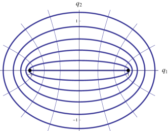
Figure 2.1: Elliptic coordinates.

Remarks 2.2.

1. In the $(q_{1},q_{2})$-plane the curves $\xi=c$ are ellipses with foci at $\pm a$, while the curves $\eta=c$ are confocal half hyperbolas, see Figure 2.1.

2. The Jacobian determinant of $G$ equals

   $$F(\xi,\eta):=\det(DG(\xi,\eta))=\sinh^{2}(\xi)+\sin^{2}(\eta)=\cosh^{2}(\xi)-\cos^{2}(\eta).$$ (2.4)

   Thus the coordinate change (2.2) is degenerate at the points $(\xi,\eta)\in\{0\}\times\{0,\pm\pi\}$ in $\overline{M}$. For $\xi=0$ the $\eta$ coordinate parametrizes the $q_{1}$-axis interval between the two centers. For $\eta=0$ ($\eta=\pm\pi$) the $\xi$ coordinate parametrizes the positive (negative) $q_{1}$-axis with $|q_{1}|>1$. $\Diamond$

2.3 Classical results

The classical analogue of (2.1) is described by the Hamiltonian function on the cotangent bundle $T^{*}Q_{2}$ of $Q_{2}:={\mathbb{R}}^{2}\setminus\{\pm a\}$ relative to the two-center potential given by:

$$H:T^{*}Q_{2}\to{\mathbb{R}}\quad\mbox{,}\quad H(p,q):=\frac{|p|^{2}}{2}+\frac{-Z_{1}}{|q-a|}+\frac{-Z_{2}}{|q+a|}.$$ (2.5)

Lemma 2.3 (see e.g. [49]).

Using $G$ defined in (2.3), and $Z_{\pm}:=Z_{2}\pm Z_{1}$, $H$ is transformed by the elliptic coordinates into

$$H\circ{(G^{-1})^{*}}(p_{\xi},p_{\eta},\xi,\eta)=\frac{1}{F(\xi,\eta)}\big{(}H_{1}(p_{\xi},\xi)+H_{2}(p_{\eta},\eta)\big{)}$$ (2.6)

where $(G^{-1})^{*}:T^{*}M\to T^{*}Q_{2}$ is the cotangential lift of $G^{-1}$, and

$$H_{1}(p_{\xi},\xi):=\frac{p_{\xi}^{2}}{2}-Z_{+}\cosh(\xi)\quad\mbox{,}\quad H_{2}(p_{\eta},\eta):=\frac{p_{\eta}^{2}}{2}+Z_{-}\cos(\eta).$$ (2.7)

There are two functionally independent constants of motion $H$ and $L:=H_{1}-\cosh^{2}(\xi)H$ with values $E$ and $K$ respectively.

Taken together, the constants of motion define a vector-valued function on the phase space of a Hamiltonian. We can study the structure of the preimages of this function (its level sets), in particular their topology. In the simplest case the level sets are mutually diffeomorphic manifolds.

Definition 2.4.

(see [1, Section 4.5]) Given two manifolds $M,N$, $f\in C^{\infty}(M,N)$ is called locally trivial at $y_{0}\in N$ if there exists a neighborhood $V\subseteq N$ of $y_{0}$ such that $f^{-1}(y)$ is a smooth submanifold of $M$ for all $y\in V$ and there there is a map $g\in C^{\infty}(f^{-1}(V),f^{-1}(y_{0}))$ such that $f\times g:f^{-1}(V)\to V\times f^{-1}(y_{0})$ is a diffeomorphism.

The bifurcation set of $f$ is the set

$${\mathcal{B}}(f):=\{y_{0}\in N\mid f\mbox{ is not locally trivial at }y_{0}\}.$$

Notice that if $f$ is locally trivial, the restriction $g{\mathbin{\upharpoonright}}\raise-2.15277pt\hbox{$\scriptstyle f^{-1}(y)$}:f^{-1}(y)\to f^{-1}(y_{0})$ is a diffeomorphism for every $y\in V$.

Remark 2.5.

The critical points of $f$ lie in ${\mathcal{B}}(f)$ (see [1, Prop. 4.5.1]), but the converse is true only in the case $f$ is proper (i.e. it has compact preimages). $\Diamond$

Define the function on the phase space as follows (omitting a projection in the second component)

$${\mathcal{F}}:=\left(\begin{smallmatrix}H\\ H_{\xi}\circ G^{*}\end{smallmatrix}\right):T^{*}Q_{2}\to{\mathbb{R}}^{2},$$ (2.8)

where $H_{\xi}(p_{\xi},\xi):=H_{1}(p_{\xi},\xi)-\cosh^{2}(\xi)E$.

Theorem 2.6 ([49]).

Let $(Z_{1},Z_{2})\in{\mathbb{R}}^{*}\times{\mathbb{R}}^{*}$, then the bifurcation set of (2.8) for positive energies equals

$${\mathcal{B}}\left({\mathcal{F}}\right)\cap\;({\mathbb{R}}_{+}\times{\mathbb{R}})=\left\{(E,K)\in{\mathcal{L}}\mid E\geq 0\text{ and }K_{+}(E)\leq K\leq K_{-}(E)\right\}.$$

Here ${\mathcal{L}}:={\mathcal{L}}_{0}\cup{\mathcal{L}}_{-}^{1}\cup{\mathcal{L}}_{-}^{2}\cup{\mathcal{L}}_{-}^{3}\cup{\mathcal{L}}_{+}^{2}\cup{\mathcal{L}}_{+}^{3}{\subset{\mathbb{R}}^{2}}$ with

$$\begin{array}[]{lcl}{\mathcal{L}}_{0}:=\{E=0\},&&{\mathcal{L}}_{-}^{1}:=\{K=Z_{-}-E\},\\ {\mathcal{L}}_{+}^{2}:=\{K=-Z_{+}-E\},&&{\mathcal{L}}_{-}^{2}:=\{K=-Z_{-}-E\},\\ {\mathcal{L}}_{+}^{3}:=\{4EK=Z_{+}^{2}\},&&{\mathcal{L}}_{-}^{3}:=\{4EK=Z_{-}^{2}\},\end{array}$$ (2.9)

and $K_{+}$ and $K_{-}$ are defined by

$$K_{+}(E):=\begin{cases}-\infty,&E>0\\ -(Z_{+}+E),&E\leq\min\left(-\frac{Z_{+}}{2},0\right)\\ \frac{Z_{+}^{2}}{4E},&0\geq E>\min\left(-\frac{Z_{+}}{2},0\right)\end{cases},$$

$$K_{-}(E):=\begin{cases}Z_{-}-E,&E\leq\frac{Z_{-}}{2}\\ \frac{Z_{-}^{2}}{4E},&E>\frac{Z_{-}}{2}\end{cases}.$$

The energies lying on the line ${\mathcal{L}}^{2}_{+}$ are the ones associated with the closed hyperbolic trajectory bouncing between the two centers [49].

Moreover, for $|Z_{+}|<Z_{-}$ the set of energy parameters included in the region $\{E\geq 0\}\cap\left\{(E,K)\in{\mathcal{L}}_{+}^{3}\;\middle|\;E<\frac{|Z_{+}|}{2}\right\}$ and contained between the curves ${\mathcal{L}}_{+}^{2}$ and ${\mathcal{L}}_{+}^{1}$ is somewhat special: on the configuration space they are associated with a family of bounded trajectories trapped near the attracting center [49].

2.4 Separation in elliptic coordinates

The importance of the change of coordinate (2.3) for the quantum problem is clarified by the following well-known theorem (see e.g. [5]). Here we enlarge the domain of $G$ to $\overline{M}$.

Theorem 2.7.

Let $u\in C_{a}({\mathbb{R}}^{2}):=\left\{u\in C({\mathbb{R}}^{2})\;\Big{|}\;u{\upharpoonright}_{{\mathbb{R}}^{2}\setminus\{\pm a\}}\text{ is twice continuously differentiable}\right\}$. The eigenvalue equation

$$\big{(}-h^{2}\Delta+V(q)\big{)}u(q)=Eu(q),\quad E\in{\mathbb{R}},$$

transformed to prolate elliptic coordinates, separates with the ansatz

$$u\circ G(\xi,\eta)=f(\xi)g(\eta)$$

into the decoupled system of ordinary differential equations

$$\begin{cases}\left(-h^{2}\partial_{\xi}^{2}-Z_{+}\cosh(\xi)-E\cosh^{2}(\xi)+\mu\right)f(\xi)=0\\ \left(-h^{2}\partial_{\eta}^{2}+Z_{-}\cos(\eta)+E\cos^{2}(\eta)-\mu\right)g(\eta)=0,\end{cases}$$

where $\mu\in{\mathbb{C}}$ is the separation constant,

$$f \in\ C^{2}_{N}([0,\infty))\ :=\left\{h\in C^{2}([0,\infty))\mid h^{\prime}(0)=0\right\},$$

$$g \in\ C^{2}_{\rm per}([-\pi,\pi])\ :=\left\{h\in C^{2}([-\pi,\pi])\mid h^{(k)}(-\pi)=h^{(k)}(\pi)\text{ for }k=0,1\right\}$$

and we have set $Z_{\pm}:=Z_{2}\pm Z_{1}$ and $\partial_{\alpha}=\frac{\partial}{\partial\alpha}$.

Remark 2.8.

Without loss we assume $Z_{-}\in[0,\infty)$ and $Z_{+}\in{\mathbb{R}}$, $Z_{+}\neq Z_{-}$, i.e. $Z_{2}\geq Z_{1}$. $\Diamond$

Remark 2.9.

Since $G$ is a diffeomorphism and since $F$ defined in (2.4) equals $\det(DG)$, the transformation to prolate elliptic coordinates $(\xi,\eta)$ defines a unitary operator

$${\mathcal{G}}:L^{2}({\mathbb{R}}^{2},dq)\to L^{2}(M,d\chi)\quad\mbox{, with}\quad d\chi:=F(\xi,\eta)\,d\xi\,d\eta.$$

$\Diamond$

Proof of 2.7. We set $r_{1}:=|q-s_{1}|$, $r_{2}:=|q-s_{2}|$ and transform to elliptic coordinates. We have

$$r_{2,1}^{2}=(q_{1}\pm 1)^{2}+q_{2}^{2}=\big{(}\cosh(\xi)\pm\cos(\eta)\big{)}^{2}.$$

Thus the distances from the centers equal

$$r_{1}=\cosh\xi-\cos\eta\quad\mbox{and}\quad r_{2}=\cosh\xi+\cos\eta.$$

For $F(\xi,\eta)=\sinh^{2}(\xi)+\sin^{2}(\eta)=\cosh^{2}(\xi)-\cos^{2}(\eta)$ we obtain

$$V\circ G(\xi,\eta)=-\frac{Z_{1}}{|q-a|}-\frac{Z_{2}}{|q+a|}={-\frac{Z_{+}\cosh(\xi)-Z_{-}\cos(\eta)}{F(\xi,\eta)}}$$

and the Laplacian $\Delta$ acts in elliptic coordinates as

$$\Delta_{{\mathcal{G}}}:=\frac{1}{F(\xi,\eta)}\left(\partial_{\xi}^{2}+\partial_{\eta}^{2}\right).$$ (2.10)

With the ansatz

$$\widetilde{u}(\xi,\eta)=f(\xi)g(\eta)\quad\mbox{ with }\quad f\in C^{2}_{N}([0,\infty))\mbox{ and }g\in C^{2}_{\rm per}([-\pi,\pi])$$

the first equation separates and we obtain the decoupled system of ordinary differential equations

$$-h^{2}\partial_{\xi}^{2}f(\xi)+\left(V_{\xi}(\xi)+\mu\right)f(\xi)=0\quad\mbox{,}\quad-h^{2}\partial_{\eta}^{2}g(\eta)+\left(V_{\eta}(\eta)-\mu\right)g(\eta)=0$$ (2.11)

where $V_{\xi}$ and $V_{\eta}$ are the multiplication operators for the functions

$$V_{\xi}(\xi):=-Z_{+}\cosh(\xi)-E\cosh^{2}(\xi)\quad\mbox{,}\quad V_{\eta}(\eta):=Z_{-}\cos(\eta)+E\cos^{2}(\eta)$$ (2.12)

∎

Remark 2.10.

Here the separation constant $\mu$ plays the role of the spectral parameter in time independent Schrödinger equations, and energy $E$ the one of a coupling constant. $\Diamond$

Proposition 2.11.

The operator ${\mathcal{H}}$ on $L^{2}({\mathbb{R}}^{2})$ defined as in (2.1) is unitarily equivalent to the operator in $L^{2}(M,d\chi)$, given by

$${\mathcal{H}}_{{\mathcal{G}}}:=-h^{2}\Delta_{{\mathcal{G}}}+V_{{\mathcal{G}}}\quad\mbox{with}\quad V_{{\mathcal{G}}}(\xi,\eta):=-\frac{Z_{+}\cosh(\xi)-Z_{-}\cos(\eta)}{F(\xi,\eta)}.$$

${\mathcal{H}}_{\mathcal{G}}$ has form core

$${\mathcal{G}}\left(C_{0}^{\infty}({\mathbb{R}}^{2})\right)=\left\{f\in C_{0}^{\infty}\left(\overline{M}\right)\mid f(\xi,\pi)=f(\xi,-\pi)\mbox{ and }\partial_{\xi}f|_{\xi=0}=0\right\}.$$

It admits a unique self-adjoint realisation with domain ${\mathcal{G}}(D({\mathcal{H}}))$ with

$$D({\mathcal{H}}):=\left\{u\in L^{2}({\mathbb{R}}^{2})\mid Vu\in L^{1}_{\rm loc}({\mathbb{R}}^{2}),\;u\in H^{1}_{\rm loc}({\mathbb{R}}^{2}),\;{\mathcal{H}}u\in L^{2}({\mathbb{R}}^{2})\right\},$$ (2.13)

where ${\mathcal{H}}u$ is to be understood in distributional sense.

Proof.

It is well-known that ${\mathcal{H}}$ has a self-adjoint realisation on $L^{2}({\mathbb{R}}^{2})$. The proof is based on the infinitesimal form boundedness of $V$ w.r.t. $\Delta$ [2, Theorem 3.2] and the KLMN Theorem [44, Theorem X.17]. In this way the operator is well-defined and has form domain $H^{1}({\mathbb{R}}^{2})$. Moreover its domain $D({\mathcal{H}})$ is given by (2.13), see [2, Theorem 3.2].

The domain of the unitarily transformed ${\mathcal{H}}_{{\mathcal{G}}}={\mathcal{G}}{\mathcal{H}}{\mathcal{G}}^{-1}$ is then transformed to ${\mathcal{G}}(D({\mathcal{H}}))$.

Finally $C_{0}^{\infty}({\mathbb{R}}^{2})$ is a form core for the quadratic form associated to ${\mathcal{H}}$, therefore it is unitarily transformed to a form core for the quadratic form associated to ${\mathcal{H}}_{\mathcal{G}}$. See [46, Section VIII.6] for the definitions. The form of the operator is given by Theorem 2.7. ∎

It is natural at this point to move our point of view from the study of ${\mathcal{H}}_{{\mathcal{G}}}-E$ on $L^{2}(M,d\chi)$ to the study of the separable operator

$$K_{E}:=K_{\xi}\otimes{\rm 1\mskip-4.0mul}+{\rm 1\mskip-4.0mul}\otimes K_{\eta}$$

acting on $L^{2}(M,d\xi\,d\eta)=L^{2}([0,\infty),d\xi)\otimes L^{2}([-\pi,\pi],d\eta)$. Here

$$\begin{split}K_{\xi}(h)&:=K_{\xi,E,h}:=-h^{2}\partial_{\xi}^{2}-Z_{+}\cosh(\xi)-E\cosh^{2}(\xi),\\ K_{\eta}(h)&:=K_{\eta,E,h}:=-h^{2}\partial_{\eta}^{2}+Z_{-}\cos(\eta)+E\cos^{2}(\eta).\end{split}$$ (2.14)

In fact, the separation reduces the problem to the study of two Sturm-Liouville equations

$$(K_{\xi}+\mu)f(\xi)=0\quad\mbox{ and }\quad(K_{\eta}-\mu)g(\eta)=0.$$ (2.15)

Following the standard convention used in the literature, we will call the first equation radial equation and the second equation angular equation. For the proper boundary conditions on $L^{2}([0,\infty),d\xi)$ respectively $L^{2}([-\pi,\pi],d\eta)$ they define essentially self-adjoint operators.

More specifically the eigenvalue equation of $K_{\eta}(h)$ is in the class of the so called Hill’s equation. In view of Proposition 2.11, we are interested in the $2\pi$-periodic solutions of the equation, i.e. we look for $g\in L^{2}([-\pi,\pi],d\eta)$ such that

$$g(-\pi)=g(\pi)\quad\mbox{and}\quad g^{\prime}(-\pi)=g^{\prime}(\pi).$$

For $K_{\xi}(h)$ it is clear that $0$ is a regular point, we will see later how to treat the singular point $\infty$ (we refer the reader to [61] for additional information concerning regular and singular points of Sturm-Liouville Problems). For what concerns the boundary conditions in $0$, as suggested by Proposition 2.11 we will require

$$f^{\prime}(0)=0.$$ (2.16)

The transformation needed to move from ${\mathcal{H}}_{\mathcal{G}}-E$ to (2.14) is obviously not unitary, as we are passing from a semibounded operator to a family of non-semibounded ones. On the other hand, their spectra are related, and we will study $\sigma({\mathcal{H}}_{\mathcal{G}})$ by means of the spectra associated to (2.14).

3 Spectrum of the angular operator and its analytic continuation

We now turn the attention to the second equation in (2.15), the angular equation. Let

$$T:=T_{\eta}(Z_{-},h,\mu,E):=h^{-2}K_{\eta}(h)-h^{-2}E,$$ (3.1)

with parameters $Z_{-}\in{\mathbb{R}}$ and $E\in(0,\infty)$. With this definition, $h^{2}[T\psi](\eta)=0$ denotes the eigenvalue equation for $K_{\eta}$.

We start considering the simpler case of equal charges ($Z_{-}=0$). Then the eigenvalue equation $[T\psi](\eta)=0$ is the Mathieu equation

$$[T\psi](\eta)=-\partial_{\eta}^{2}\psi(\eta)-\frac{2\mu-E}{2h^{2}}\psi(\eta)+2\frac{E}{4h^{2}}\cos(2\eta)\psi(\eta)=0$$ (3.2)

with periodic boundary conditions in $[-\pi,\pi]$. We apply Floquet theory (see [16, 37, 41, 55]), using the fundamental matrix

$${\mathcal{F}}(\lambda,\delta):=\left(\begin{smallmatrix}f_{1}&f_{2}\\ f_{1}^{\prime}&f_{2}^{\prime}\end{smallmatrix}\right)(\pi;\lambda,\delta),\qquad\lambda:=\frac{2\mu-E}{2h^{2}},\;\delta:=\frac{E}{4h^{2}},$$ (3.3)

built from the fundamental system of solutions $\eta\mapsto f_{i}(\eta;\lambda,\delta)$, with

$$f_{1}(0;\lambda,\delta)=1=f_{2}^{\prime}(0;\lambda,\delta)\quad\mbox{,}\quad f_{2}(0;\lambda,\delta)=0=f_{1}^{\prime}(0;\lambda,\delta)$$ (3.4)

(henceforth the prime ^′ means the partial derivative w.r.t. the first variable). The potential $V(\eta):=\cos(2\eta)$ being even, it follows that all the $2\pi$-periodic solutions must be either $\pi$-periodic or $\pi$-antiperiodic in $[0,\pi]$ (or $[-\pi,0]$).

The structure of the periodic solutions and their eigenvalues for the Mathieu equation is well-understood (see [41, Chapter 2]): For each integer $n\geq 0$ one finds two solutions $\operatorname{ce}_{n}(\bullet;\delta)$ and $\operatorname{se}_{n+1}(\bullet;\delta)$, called Mathieu Cosine and Mathieu Sine respectively, that have exactly $n$ zeroes in $(0,\pi)$ and that are $\pi$-periodic for even $n$ and $\pi$-antiperiodic for odd $n$, the corresponding eigenvalues being $\lambda^{+}_{n}(\delta)$ and $\lambda^{-}_{n+1}(\delta)$ respectively. For parameter values $E\in{\mathbb{R}}$, $\delta\in(0,\infty)$ the $\lambda^{+}_{n}$ and $\lambda^{-}_{n+1}$ are real and

$$\lambda^{+}_{0}<\lambda^{-}_{1}<\lambda^{+}_{1}<\lambda^{-}_{2}<\lambda^{+}_{2}<\cdots.$$

The following facts are proved in [30, Chapter VII.3.3], [40, Chapter 2.4], [41, Chapter 2.2] and [58].

1. The eigenvalues of the Mathieu operators are real-analytic functions in $\delta\in{\mathbb{C}}$, whose algebraic singularities all lie at non-real branch points.

2. They can be defined uniquely as functions $\lambda^{\pm}_{n}(\delta)$ of $\delta$ by introducing suitable cuts in the $\delta$-plane. Moreover they admit an expansion in powers of $\delta$ with finite convergence radius $r_{n}$ such that $\liminf_{n\to\infty}\frac{r_{n}}{n^{2}}\geq C$ for some $C>0$.

3. The number of branch points is countably infinite, and there are no finite limit points.

4. The operator $T$ corresponding to (3.2) can be decomposed according to

   $$L^{2}([-\pi,\pi])=L_{0}^{+}\oplus L_{1}^{+}\oplus L_{0}^{-}\oplus L_{1}^{-}$$

   where the superscripts $\pm$ denote respectively the sets of even and odd functions and where the subscripts $0$ and $1$ denote respectively the sets of functions symmetric and antisymmetric with respect to $x=\pi/2$.

5. The restrictions of $T$ to the four subspaces $L^{\pm}_{0/1}$ are self-adjoint and have only simple eigenvalues, as given by the following scheme:

   $$L_{0}^{+} \;:\;\lambda_{n}^{+},\psi_{n}^{+},\qquad n=0,2,4,6,\ldots;$$

   $$L_{1}^{+} \;:\;\lambda_{n}^{+},\psi_{n}^{+},\qquad n=1,3,5,\ldots;$$

   $$L_{0}^{-} \;:\;\lambda_{n}^{-},\psi_{n}^{-},\qquad n=1,3,5,\ldots;$$

   $$L_{1}^{-} \;:\;\lambda_{n}^{-},\psi_{n}^{-},\qquad n=2,4,6,\ldots.$$

6. All the eigenvalues in each of the four groups of the previous remark belong to the same analytic function, i.e. the eigenvalues in the same group lie on the same Riemann surface [41, 59].

7. The eigenfunctions $\eta\mapsto\psi_{n}^{\pm}(\eta)$ are themselves analytic functions of $x$ and $\delta$. For all $n\in{\mathbb{N}}$ they coincide with the Mathieu Cosine and the Mathieu Sine introduced above, namely $\psi_{n}^{+}\equiv\operatorname{ce}_{n}$ and $\psi_{n+1}^{-}\equiv\operatorname{se}_{n+1}$ ($n\in{\mathbb{N}}_{0}$).

Despite the completeness and the clarity of perturbation theory for one-parameter analytic families of self-adjoint operators, the situation is much more intricate and much less complete in presence of more parameters. On the other hand we can use our restrictions on the parameters and the special symmetries of the potential to play in our favor.

For a general value of $Z_{-}$, the eigenvalue equation is

$$[T\psi](\eta)=-\partial_{\eta}^{2}\psi(\eta)+\left(\frac{Z_{-}}{h^{2}}\cos(\eta)+\frac{E}{2h^{2}}\cos(2\eta)-\frac{2\mu-E}{2h^{2}}\right)\psi(\eta)=0,$$ (3.5)

with periodic boundary conditions on $[-\pi,\pi]$ and eigenvalue $\mu$. Let us call

$$\lambda:=\frac{2\mu-E}{2h^{2}},\qquad\gamma_{1}:=\frac{Z_{-}}{h^{2}},\qquad\gamma_{2}:=\frac{E}{2h^{2}}.$$ (3.6)

Notice that the main difference between (3.5) and the Mathieu equation is that now the period of the potential is no more smaller than the length of the considered interval. Thus, in applying Floquet theory we do not anymore look for solutions which are (anti-)periodic under translation by $\pi$.

Remark 3.1.

By standard Sturm-Liouville theorems (see for instance [16, Theorems 2.3.1 and 3.1.2]) we know that for every choice of $\gamma_{1}$ and $\gamma_{2}$ the spectrum of $K_{\eta}(h)$ is discrete, at most doubly degenerate and accumulates only at infinity. Anyhow it follows from [37, Theorem 7.10] using a change of variable that in this case there cannot be coexistence of $2\pi$-periodic eigenfunctions for the same eigenvalue. Thus the spectrum is non-degenerate. $\Diamond$

It is proved in [54] that, for real-valued $E$ and $Z_{-}$, the eigenvalues of $h^{-2}K_{\eta}(h)$ form a countably infinite set $\{\lambda_{n}(\gamma_{1},\gamma_{2},h)\}_{n\geq 0}$ of transcendental real analytic (actually entire) functions of the parameters $\gamma_{1},\gamma_{2}\in{\mathbb{R}}$, so that in the $(\gamma_{1},\gamma_{2},\lambda)$ space the sets

$$\left\{\left(\gamma_{1},\gamma_{2},\lambda_{n}(\gamma_{1},\gamma_{2})\right)\mid(\gamma_{1},\gamma_{2})\in{\mathbb{R}}^{2}\right\}$$

define a countably infinite number of uniquely defined real-analytic surfaces.

We can apply analytic perturbation theory [30, Chapter VII] to

$$T(\beta):=T+\beta(1+\cos(2\eta))$$

where $T$ is defined in (3.1) and $\beta$ is assumed to be defined by $h$ and some real parameter $E_{\rm im}$ as follows

$$\beta(E_{\rm im},h):=i\frac{E_{\rm im}}{2h^{2}}\qquad(\text{with }i=\sqrt{-1},\;h\in(0,\infty)).$$

Therefore $T(\beta)$ is merely (3.5) with complex $E$. It is evident that $T(\beta)$ defines a self-adjoint analytic family of type (A) in the sense of Kato. Therefore [30, Chapter VII] each $\lambda_{n}(\gamma_{1},\gamma_{2},\beta)$ admits an analytic extension on the complex plane around each real $E$ that can be expanded as a series in $\beta=iE_{\rm im}/2h^{2}$ with an $n$-dependent convergence radius $\rho_{n}$. Remark 3.1 concerning the simplicity of the spectrum and the construction described at points 4. and 5. on page 4 is still valid. Therefore we may continue to regard each eigenvalue as simple restricted on its proper subspace and consider the lower bound of the convergence radius in terms of the eigenvalues’ spacing in the proper subspace. These distances are known to be at least of order $n$, in the sense that there exists $C>0$ such that $\liminf_{n\to\infty}\frac{n\text{th-distance}}{n}\geq C$, see [30, Chapter VII.2.4].

In the particular case considered, we can use the ansatz given by [37, Theorem 1.1] to bound the distance between the periodic solutions with a boundary-value problem. To this end we can use the discussion of [57, Section 5] and apply it to our case to obtain the following rough estimate, generalizing point (2) on page 2.

Theorem 3.2.

Let $E>2|Z_{-}|$. Then the convergence radii $\rho^{D,N}_{n}$ corresponding to (3.5) with Dirichlet (resp. Neumann) boundary conditions satisfy

$$\liminf_{n\to\infty}\;\frac{\rho^{D,N}_{n}}{n^{2}}\geq\frac{6}{13}$$

Proof.

In [57], Section 5, it is shown that a result like our Theorem 3.2 holds for the Mathieu equation (see [57, Theorem 5.1]). This is a particular case of a more general theorem on the quadratic growth of the convergence radii for the eigenvalues of a big family of differential equations (see [57, Theorem 3.4]).

To apply [57, Theorem 3.4] and obtain the theorem for the Mathieu equation, it is enough to check the assumptions and use the estimates obtained there to get the constants in the growth rate. This check relies on some crude estimates on incomplete elliptic integrals and on the potential that can be used also for our problem.

Indeed, we can replace the estimate $|2\cos(2z)|\leq 2\cosh(2\Im z)$ for the Mathieu potential by a corresponding estimate for $\cos(2x)+\frac{Z_{-}}{2E}\cos(x)$: if $E\gg|2Z_{-}|$, then

$$\left|\cos(2z)+2\frac{Z_{-}}{E}\cos(z)\right|\leq 2\cosh(2\Im z).$$

Then, the constants in the proof of [57, Theorem 5.1], would coincide with the constants obtained for our potential: $R=2\cosh(2\delta)$, $R_{0}=2$, $U^{2}=\frac{\pi^{2}}{16}+\delta^{2}$ (notation from [57, Section 5]). And choosing $\delta=\frac{1}{2}$ one can check that the assumptions of [57, Theorem 3.4] are satisfied and the growth constant is $\frac{6}{13}$ also in this case. ∎

Remark 3.3.

As for [57, Theorem 5.1], we used very crude estimates. The constants, and in particular the lower bound for the growth rate, are far from being optimal also in this case and could be improved following the enhancements presented in [58].

Remark 3.4.

We expect that Theorem 3.2 still holds true for $0<E\leq 2|Z_{-}|$. $\Diamond$

4 Asymptotic behaviour of solutions of the radial Schrödinger equation and their analytic extensions

The general estimates that we develop in this section are needed in order to justify the formal step in the separation of variables and the construction of the Green’s functions. We proceed with a philosophy close to the one of [3].

With the substitution $E=k^{2}$ of its parameter, the radial equation in (2.15) takes the form

$$v^{\prime\prime}(\xi,k)+h^{-2}\left(k^{2}\cosh^{2}(\xi)+Z_{+}\cosh(\xi)-\mu\right)v(\xi,k)=0$$ (4.1)

where $\xi>0$, $h>0$ and $k\in{\mathbb{C}}$ are arbitrary. Now for $l\in{\mathbb{N}}$ we set $\mu:=\mu_{l}$, the $l$-th eigenvalue of $K_{\eta}$ (counted in ascending order for real parameters and then extended analytically). We assume w.l.o.g. that $h=1$, since $h$ can be absorbed in the other parameters.

We will be interested in the solutions $v_{\pm}(\xi,k):=v_{\pm}(\xi,k,\mu)$ of (4.1) which decay as $\xi\to\infty$ for $k$ in the upper, resp. lower, half-plane ${\mathbb{C}}_{\pm}=\{k\in{\mathbb{C}}\mid\Im(k)\lessgtr 0\}$. We call them, following [3] “outgoing”, resp. “incoming”, and we will make a specific choice of such a family of solutions by fixing the behaviour of $v_{\pm}(\xi,k)$ as $\xi\to\infty$.

We want to construct a phase function that is an approximate solution of the eikonal equation for the Schrödinger equation (4.1), that is characterized by a particular asymptotic behaviour and that is analytic in $k$. We would like to consider something of the form

$$\phi(\xi,k)\sim\int_{0}^{\xi}\sqrt{k^{2}\cosh^{2}(t)+Z_{+}\cosh(t)-\mu}\;dt,$$ (4.2)

but this gives a well-defined analytic function only for $|k|^{2}>|Z_{+}-\mu|$. For our analysis it will be essential that the phase function is analytic in $k\in{\mathbb{C}}\setminus\{0\}$. To construct it we reconsider the previous ansatz and perform a change of variables. If we call $\tau=\sinh(t)$, the above equation is transformed into

$$\phi(\xi,k)\sim\int_{0}^{\sinh(\xi)}\sqrt{k^{2}-q(\tau)}\;d\tau\quad\mbox{with}\quad q(\tau):=\frac{\mu}{1+\tau^{2}}-\frac{Z_{+}}{\sqrt{1+\tau^{2}}}.$$ (4.3)

If we call $r=\sinh(\xi)$, we may consider the map $r\mapsto\phi(\operatorname{arcsinh}(r),k)$ to be the phase function of a long-range potential, asymptotic to $r\mapsto kr$ as $r\to\infty$, (see (4.7) for a more precise statement), plus a short-range perturbation.

4.1 Decomposition into long and short range

To construct the phase function $\phi$, we introduce an appropriate decomposition of the potential $q$ into short and long range parts.

Let $j\in{\mathbb{N}}$. We define $l_{j},s_{j}\in(0,\infty)\to{\mathbb{R}}$ by

$$s_{j}(\tau):=q(\tau)-l_{j}(\tau)\quad\mbox{and}\quad l_{j}(\tau):=-\chi(\tau)\frac{Z_{+}}{\sqrt{1+\tau^{2}}},$$ (4.4)

where $\chi(\tau)=1$ if $Z_{+}\geq 0$ and otherwise is defined as follows: $\chi\in C_{c}^{\infty}((0,\infty);[0,1])$ such that $\chi(\tau)=0$ if $\tau\leq j|Z_{+}|$ and $\chi(\tau)=1$ if $\tau\geq j|Z_{+}|+1$.

Note that $s_{j}(\tau)\in L^{1}((0,\infty))$, $l_{j}\in C^{2}((0,\infty))$,

$$\sup_{\tau>0}l_{j}(\tau)\leq 1/j\quad\mbox{and}\quad l_{j}(\tau)=-\frac{Z_{+}}{\sqrt{1+\tau^{2}}}\text{ for }\tau>R_{j},$$

for $R_{j}:=j|Z_{+}|+1$.

Let $\Omega_{j}:=\{k\in{\mathbb{C}}\mid|k|^{2}>1/j\}$ and $\phi_{j}\in(0,\infty)\times\Omega_{j}\to{\mathbb{C}}$, defined by

$$\phi_{j}(\xi,k):=\int_{0}^{\sinh(\xi)}\sqrt{k^{2}-l_{j}(\tau)}\;d\tau.$$ (4.5)

Here we have taken the principal branch of the square root, i.e. the uniquely determined analytic branch of $\sqrt{z}$ that maps $(0,\infty)$ into itself.

Note that $\phi_{j}(\xi,\cdot)$ is analytic in $\Omega_{j}$ and $\phi_{j}(\cdot,k)\in C^{2}((0,\infty))$. Furthermore, for $k\in\Omega_{j}$, $\phi_{j}(\cdot,k)$ satisfies the eikonal equation

$$|\partial_{\xi}\psi(\xi)|^{2}=k^{2}-l_{j}(\sinh(\xi))$$ (4.6)

on $(0,\infty)$.

Theorem 4.1.

Let

$$D:=\{(\xi,k)\in(0,\infty)\times{\mathbb{C}}\setminus\{0\}\mid\sinh(\xi)\geq|k^{-2}Z_{+}|+1\}.$$

There exist a function $\phi:D\to{\mathbb{C}}$ satisfying the following properties:

1. For all $(\xi,k)\in D$, $\phi(\xi,-k)=-\phi(\xi,k)$.

2. For all $j\in{\mathbb{N}}$, the restriction of $\phi-\phi_{j}$ to $(R_{j},\infty)\times\Omega_{j}$ doesn’t depend on $\xi$ and is an analytic function of $k$.

3. For all $k\in{\mathbb{C}}\setminus\{0\}$, $\phi(\xi,\cdot)$ is analytic on each $\Omega_{j}$, for $j\in{\mathbb{N}}$ such that $\sinh(\xi)>R_{j}$.

4. For all $k\in{\mathbb{C}}\setminus\{0\}$, $\phi(\cdot,k)\in C^{2}((0,\infty))$ and satisfies the eikonal equation (4.6) on $(R_{j},\infty)$ where $j$ is the integer part of $|k^{2}|^{-1}$.

The theorem follows from the construction above with the same proof as [3, Proposition 2.1].

Remark 4.2.

The phase function $\phi$ defined in the previous theorem is not unique. This is, however, immaterial for our purposes. In fact, our main concern is to have a controlled behaviour, as $\xi\to\infty$ (see Proposition 4.3) and good analyticity properties in order to identify the two (unique) waves $v_{\pm}$ for a wide range of parameters.

Henceforth we will refer to the $\phi(\xi,k)$ defined in Theorem 4.1 as a global phase function.

Proposition 4.3.

The global phase function $\phi(\xi,k)$ has the asymptotic behaviour given by

$$\phi(\xi,k)=k\sinh(\xi)+\frac{Z_{+}}{2k}\xi+{\cal O}(1)=\frac{k}{2}e^{\xi}\big{(}1+o(1)\big{)}\quad\mbox{as}\quad\xi\to\infty.$$ (4.7)

Remark 4.4.

In the proposition the term $s(\tau):=\frac{\mu}{1+\tau^{2}}$ has been dropped out. In fact it belongs to the short range component $s_{j}$ of (4.4) and choosing in (4.4) a different decomposition of $q(\tau)$ into a short-range and long-range part, keeping $l(\xi)$ fixed near infinity, modifies $\phi(\xi,k)$ by an analytic function of $k$ alone. $\Diamond$

Proof.

Without losing generality we can suppose $|k|>|Z_{+}|$ and consider the simplified phase function

$$\phi(\xi,k):=\int_{0}^{\xi}\sqrt{k^{2}\cosh^{2}(t)+Z_{+}\cosh(t)}\;dt=k\int_{{}_{0}}^{\xi}\cosh(t)\sqrt{1+\frac{Z_{+}}{k^{2}\cosh(t)}}\;dt$$ (4.8)

as $\xi\to\infty$:

$$\phi(\xi,k)={} k\int_{0}^{\xi}\cosh(t)\left(1+\frac{Z_{+}}{2k^{2}\cosh(t)}+{\cal O}\left(k^{-2}\cosh^{-2}(t)\right)\right)\;dt$$

$$={} k\sinh(\xi)+\frac{Z_{+}}{2k}\xi+{\cal O}(1),$$

Writing $\sinh(\xi)=(e^{x}-e^{-x})/2$ and collecting the growing term we have the thesis. ∎

The Liouville-Green Theorem [17, Corollary 2.2.1] guarantees that for each $k\in{\mathbb{C}}$ there exist two linearly independent solutions of (4.1) whose asymptotics as $\xi\to\infty$ is given by

$$y_{1,2}(\xi)=\textstyle{\frac{1}{\sqrt{\phi^{\prime}(\xi,k)}}}\exp\big{(}{\pm i\phi(\xi,k)}\big{)}\big{(}1+o(1)\big{)}\quad\text{ for }\xi\to\infty.$$

In particular, it follows from the asymptotic estimate of Proposition 4.3 that (4.1) must be in the Limit Point Case at infinity (more precisely Case I of [9, Theorem 2.1]) if we set $r(x):=\cosh^{2}(x)$, $p:=1$ and $\lambda:=k^{2}$. In what follows we investigate the regularity of the solutions with respect to $\xi$ and $k$.

Theorem 4.5 (Outgoing and incoming solutions).

For each $k\in{\mathbb{C}}\setminus\{0\}$, equation (4.1) has unique solutions $v_{\pm}(\xi,k)$ verifying the asymptotic relation

$$v_{\pm}(\xi,k)=\sqrt{2}e^{-\frac{\xi}{2}}\exp\big{(}\pm i\phi(\xi,k)\big{)}\big{(}1+o(1)\big{)}\quad\mbox{ as}\quad\xi\to\infty.$$ (4.9)

(4.9) holds uniformly in any truncated cone

$$\Lambda_{\pm}(\eta,\delta)\,:=\{k\in{\mathbb{C}}\setminus\{0\}\mid\eta\leq\arg(\pm k)\leq\pi-\eta,\;|k|\geq\delta\}\quad\mbox{with}\quad\eta\geq 0,\ \delta>0.$$

The family of solutions $k\mapsto v_{\pm}(\xi,k)$ defined by (4.9) is analytic in the half planes $k\in{\mathbb{C}}_{\pm}$ pointwise in $\xi$, and extends continuously to $k\in\overline{{\mathbb{C}}}_{\pm}\setminus\{0\}$.

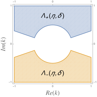
Figure 4.1: Cones $\Lambda_{\pm}$ for $\eta=1/3$ and $\delta=1/2$.

Remark 4.6.

(1) and the uniqueness of Theorem 4.5 imply that $v_{+}(\xi,k)=v_{-}(\xi,-k)$. In particular it suffices to consider $v_{+}$. $\Diamond$

Proof.

In view of Theorem 4.1 and the subsequent remark, we can reduce the proof to the case where the phase function $\phi$ is given by (4.8) for $\xi>0$ and $|k|^{2}>|Z_{+}|$. We call $\phi$ a local phase function. Let

$$V_{\pm}(\xi,k):=\left(\frac{k}{\partial_{\xi}\phi(\xi,k)}\right)^{\frac{1}{2}}e^{\pm i\phi(\xi,k)}$$ (4.10)

define the approximate solutions of (4.1).

For $|k|\geq\delta$ the function $V_{\pm}$ satisfies the comparison equation

$$V^{\prime\prime}_{\pm}(\xi,k)+\left(k^{2}\cosh^{2}(\xi)+Z_{+}\cosh(\xi)+{\textstyle\frac{1}{2}}S\phi(\xi,k)\right)V_{\pm}(\xi,k)=0$$ (4.11)

where $S\phi$ denotes the Schwarzian derivative

$$S\phi=\frac{\phi^{\prime\prime\prime}}{\phi^{\prime}}-\frac{3}{2}\left(\frac{\phi^{\prime\prime}}{\phi^{\prime}}\right)^{2}$$ (4.12)

w.r.t. $\xi$. For $k\in\Lambda_{\pm}(\eta,\delta)$ we consider the inhomogeneous Volterra Integral Equation [56]

$$v_{\pm}(\xi,k)=V_{\pm}(\xi,k)-\int_{\xi}^{\infty}K_{k}(\xi,t)F_{k}(t)v_{\pm}(t,k)\;dt$$ (4.13)

where $F_{k}(t)=\frac{1}{2}S\phi(t,k)+\mu$ is the function that expresses the difference between the Schrödinger equation (4.1) and the comparison equation (4.11) and $K(\xi,t)$ is the Green’s function associated with equation (4.10):

$$K(\xi,t)=W(V_{-},V_{+})^{-1}\left\{V_{+}(\xi)V_{-}(t)-V_{+}(t)V_{-}(\xi)\right\}$$ (4.14)

(the parameter $k$ being suppressed), with Wronskian $W(V_{-},V_{+}):=V_{-}V_{+}^{\prime}-V_{-}^{\prime}V_{+}=2ik$.

To give (4.13) meaning we need to check if the definition makes sense and a solution can be found.

We explicitly compute $S\phi$ and thus $F$ using (4.12), obtaining

$$S\phi\,(\xi)=\frac{10k^{4}-Z_{+}^{2}-2k^{4}\cosh(2\xi)+Z_{+}\operatorname{sech}(\xi)\left(12k^{2}+5Z_{+}\operatorname{sech}(\xi)\right)}{8\left(Z_{+}+k^{2}\cosh(\xi)\right)^{2}}$$

and thus, for real $\xi$ and for every $k\in\Lambda_{+}(\eta,\delta)$, we have

$$\lim_{\xi\to\infty}|F(\xi)|={\textstyle\frac{1}{8}}+\mu\quad\mbox{ and }\quad C_{F}:=\sup_{\xi\in(0,\infty)}|F(\xi)|<\infty.$$ (4.15)

Of course $C_{F}$ depends on $Z_{+}$, $\mu$ and $k$, thus on $\eta$ and $\delta$. Moreover from (4.10) and (4.7), writing $k\in\Lambda_{+}(\eta,\delta)$ as $k=k_{r}+ik_{i}$ ($k_{r},\,k_{i}$ real), we get

$$\left|V_{\pm}(\xi,k)\right|=\sqrt{2}e^{-\frac{\xi}{2}}(1+o(1))\left|e^{ik\left(\frac{\phi(\xi,k)}{k}\right)}\right|\leq C_{V}e^{-\frac{\xi}{2}}\exp\big{(}{-\textstyle\frac{k_{i}}{2}e^{\xi}(1+o(1)\big{)}},$$ (4.16)

where $\displaystyle C_{V}(k):=\sup_{\xi\in(0,\infty)}\left(e^{\xi/2}|k/\phi^{\prime}(\xi,k)|\right)<\infty$ by (4.8). Therefore for $0<\xi\leq t<\infty$ we have

$$\left|K(\xi,t)\right|={} \left|\frac{1}{2ik}\sqrt{\frac{k^{2}}{\phi^{\prime}(t,k)\phi^{\prime}(\xi,k)}}\left(e^{i(\phi(\xi,k)-\phi(t,k))}-e^{i(\phi(t,k)-\phi(\xi,k))}\right)\right|$$

$$\leq{} \frac{C_{V}^{2}}{2}e^{-\frac{\xi+t}{2}}C_{K}\left|\textstyle\exp\left(-ik\int_{\xi}^{t}\cosh(\tau)\sqrt{1+\frac{Z_{+}}{k^{2}\cosh(\tau)}}\,d\tau\right)\right|,$$ (4.17)

where

$$C_{K}(k):=\displaystyle\sup_{t,\xi\in{\mathbb{R}}^{+}}\left|1-\textstyle\exp\left(2ik\int_{\xi}^{t}\cosh(\tau)\sqrt{1+\frac{Z_{+}}{k^{2}\cosh(\tau)}}\,d\tau\right)\right|\leq 2.$$

It follows from (4.15), (4.16) and (4.17) that the Volterra Integral Equation (4.13) is well-defined as a mapping from the function space

$${\mathcal{C}}_{\pm}(\eta,\delta):=\Big{\{}f\in C^{2}\big{(}(0,\infty)\times\Lambda_{\pm}(\eta,\delta)\big{)}\Big{|}\,\forall k\in\Lambda_{\pm}(\eta,\delta),\|f\|_{k}:=\!\sup_{x\in(0,\infty)}\!\left|f(x,k)\,e^{\mp i\phi(x,k)}\right|<\infty\Big{\}}$$ (4.18)

to itself. In particular, being $V_{\pm}\in{\mathcal{C}}_{\pm}(\eta,\delta)$ we can apply the Picard iteration procedure to find a solution of the equation and prove its existence. We claim that the solution must be unique. Suppose that there exists two solutions $v_{+},\tilde{v}_{+}\in{\mathcal{C}}_{+}$ of (4.13), then

$$\psi(\xi,k):=v_{+}(\xi,k)-\tilde{v}_{+}(\xi,k)=-\int_{\xi}^{\infty}K(\xi,t)F(t)\psi(t,k)\;dt.$$ (4.19)

At this stage, it is not obvious that the r.h.s. of (4.13) is a contraction, that would allow us to conclude the proof in a standard way. In the rest of the proof we show that for appropriate initial values this is indeed the case, therefore proving the unicity and the uniformity of the estimates. The previous estimates applied to (4.19) give

$$\left|\psi(\xi,k)\right|={} \left|\int_{\xi}^{\infty}K(\xi,t)F(t)\psi(t,k)\;dt\right|\leq\int_{\xi}^{\infty}\left|K(\xi,t)F(t)\psi(t,k)\right|\;dt$$

$$\leq{} \frac{C_{K}C_{F}C_{\psi}}{2}\left|\sqrt{\frac{k}{\phi^{\prime}(\xi,k)}}\right|\left|e^{i\phi(\xi,k)}\right|\int_{\xi}^{\infty}\left|\sqrt{\frac{k}{\phi^{\prime}(t,k)}}\right|\;dt$$

$$\leq{} \frac{C_{K}C_{F}C_{\psi}C_{V}}{2}e^{-\frac{\xi}{2}}\left|e^{i\phi(\xi,k)}\right|\int_{\xi}^{\infty}\sqrt{2}e^{-\frac{t}{2}}(1+o(1))\;dt$$

$$\leq{} \frac{C_{K}C_{F}C_{\psi}C_{V}C_{I}}{2}e^{-\frac{\xi}{2}}\left|e^{i\phi(\xi,k)}\right|\int_{\xi}^{\infty}e^{-\frac{t}{2}}\;dt=C_{\psi}C_{\rm tot}e^{-\xi}\left|e^{i\phi(\xi,k)}\right|$$ (4.20)

where $C_{\psi}(k):=\|\psi\|_{k}$, $C_{I}:=\sup_{\xi\in(0,\infty)}\sqrt{2}\left((1+e^{-2\xi})\sqrt{1+\frac{Z_{+}}{k^{2}\cosh(\xi)}}\right)^{-\frac{1}{2}}$ and $C_{\rm tot}:=C_{K}C_{F}C_{V}C_{I}$. Using equations (4.19) and (4.20) we can reiterate the procedure, in fact defining

$$\psi_{1}(\xi,k):=\int_{\xi}^{\infty}K(\xi,t)F(t)\psi(t,k)\;dt\quad\mbox{and}\quad\psi_{n}(\xi,k):=\int_{\xi}^{\infty}K(\xi,t)F(t)\psi_{n-1}(t,k)\;dt,$$

one can prove by induction that

$$\left|\psi(\xi,k)\right|=\left|\psi_{n}(\xi,k)\right|\leq\frac{\;C^{n}_{\rm tot}\;e^{-n\xi}}{(2n-1)(2n-3)\cdots 3\cdot 1}\left|e^{i\phi(\xi,k)}\right|\leq C_{\psi}\frac{C^{n}_{\rm tot}\;e^{-n\xi}}{n!}\left|e^{i\phi(\xi,k)}\right|$$ (4.21)

uniformly in $k\in\Lambda_{+}(\eta,\delta)$ and for all $n\in{\mathbb{N}}$. The convergence of

$$\sum_{n=1}^{\infty}C_{\psi}\frac{C^{n}_{\rm tot}}{n!}e^{-n\xi}\left|e^{i\phi(\xi,k)}\right|=C_{\psi}\left|e^{i\phi(\xi,k)}\right|\left(e^{C_{\rm tot}e^{-\xi}}-1\right)$$ (4.22)

implies that $\left|\psi(\xi,k)\right|=0$, i.e. $\tilde{v}_{+}=v_{+}$.

The same inequality implies that after some iterates the homogeneous integral equation is a contraction, and coupled with the bounds on $V_{+}$ it implies that (4.13) has a unique fixed point. This proves the existence and uniqueness of the solution. In fact if we define

$$v_{0,+}(\xi,k):=V_{+}(\xi,k)\quad\mbox{,}\quad v_{n,+}(\xi,k):=-\int_{\xi}^{\infty}K(\xi,t)F(t)v_{n-1,+}(t,k)\;dt,$$

the Picard iteration converges to $v_{+}=\sum_{n=0}^{\infty}v_{n,+}$, and the series converges absolutely uniformly in $k\in\Lambda_{+}(\eta,\delta)$ with $\left|v_{+}(\xi,k)\right|\leq\left|V_{+}(\xi,k)\right|e^{Ce^{-\xi}}$ for some positive constant $C$. Therefore one has

$$v_{+}(\xi,k)=V_{+}(\xi,k)(1+o(1))\quad\mbox{ as }\quad\xi\to\infty$$

and (4.9) holds.

The fact that all the bounds are valid for $k\in{\mathbb{R}}$ completes the proof. ∎

Remark 4.7.

It is possible to compute an explicit bound like (4.21) using the fact that

$$\left|v_{n,+}(\xi)\right|\leq C_{V}e^{-\frac{\xi}{2}}\left|e^{i\phi(\xi,k)}\right|\frac{C_{\rm tot}^{n}e^{-n\xi}}{2^{n}n!}.$$

In particular the dependence on $\mu$, the parameter of the short-range potential in (4.3), appears in the constant $C_{\rm tot}$. In view of the previous estimates it can be bounded by $|\mu|{\cal O}(1)$. Therefore we can be more precise and estimate

$$v_{\pm}(\xi,k)=\sqrt{2}e^{-\frac{\xi}{2}}e^{\pm i\phi(\xi,k)}\big{(}1+M_{\pm}(\xi,k,\mu)\big{)}\quad\mbox{ as }\quad\xi\to\infty,$$ (4.23)

where for some constant $C\neq 0$ we have $M_{\pm}(\xi,k,\mu)=e^{C|\mu|e^{-\xi}}o(1)$. $\Diamond$

Remark 4.8.

Let $w$ be any other family of solutions of (4.1), analytic in $k\in{\mathbb{C}}\setminus\{0\}$ and satisfying for $k\in\Lambda_{+}(\eta,\delta)$ the estimate $w(\xi,k)=o(1)$ as $\xi\to\infty$. Then

$$w(\xi,k)=\gamma(k)v_{+}(\xi,k),$$

where $\gamma(k)$ is a nowhere-vanishing analytic function of $k\in\Lambda_{+}(\eta,\delta)$. $\Diamond$

Remark 4.9.

In case $Z_{+}=0$, the solutions of $\eqref{eq:schro}$ are given by linear combinations of the modified Mathieu functions (${\rm Mc}$ and ${\rm Sc}$) [18, §16.6]. In particular, if we look at their asymptotic behaviour, we find out that up to a constant factor

$$v_{+}(\xi,k)={\rm Mc}\left(\mu-\frac{k^{2}}{2},\frac{k^{2}}{4},\xi\right)$$ (4.24)

where ${\rm Mc}(a,q,x)$ is the modified Mathieu cosine, i.e. the solution of

$$y^{\prime\prime}(x)-(a-2q\cosh(2x))y(x)=0$$

that decays for $\sqrt{q}\in{\mathbb{C}}_{+}$. It is well-known [41, Chapter 2] that the function in the RHS of (4.24) admits an analytic continuation through the positive real axis on the negative complex plane for $-\pi/2\leq\arg(k)\leq\pi/2$ and that for $x\to\infty$ and $k\in{\mathbb{C}}_{+}$ it has the following asymptotic behaviour [18, 41]

$${\rm Mc}\left(\mu-\frac{k^{2}}{2},\frac{k^{2}}{4},x\right)=e^{-\frac{x}{2}}\exp\big{(}{i{\textstyle\frac{k}{2}}e^{x}(1+o(1))}\big{)}\big{(}1+o(1)\big{)},$$

in line with the estimates (4.7) and (4.9), valid for all $Z_{+}$. $\Diamond$

For what follows we will need to work in a slightly different setting. If we perform the change of variable defined by $\xi\mapsto{\operatorname{Log}}(x+1)$ (with the principal branch ${\rm Log}$ of the logarithm), for $\tilde{v}(x,k):=v(\operatorname{Log}(x+1),k)$  Equation (4.1) takes the form

$$\begin{split}\left((x+1){\tilde{v}}^{\prime}(x,k)\right)^{\prime}&+h^{-2}\,q(x,k,Z_{+},\mu)\,{\tilde{v}}(x,k)=0\qquad\mbox{with}\\ q(x,k,Z_{+},\mu):=&\frac{k^{2}}{4}\left(x+1+2(x+1)^{-1}+(x+1)^{-3}\right)+\frac{Z_{+}}{2}\left(1+(x+1)^{-2}\right)-\frac{\mu}{x+1}.\end{split}$$ (4.25)

where $x>0$, $h>0$ and $k\in{\mathbb{C}}\setminus\{0\}$. As before we assume $h=1$ for the moment.

Remark 4.10.

In this case Theorem 4.5 and Remark 4.8 is still valid and in accord with the Liouville-Green Theorem we have two unique solutions that as $x\to\infty$ are asymptotic to

$$\begin{split}{\tilde{v}}_{\pm}(x,k)={}&\frac{1}{\sqrt{x+1}}e^{\pm i\Psi(x,k)}(1+o(1))\\ ={}&\frac{1}{\sqrt{x+1}}\textstyle\exp\left(\pm i\left(\frac{k}{2}x+\frac{Z_{+}}{2k}\log(x+1)+\frac{k}{2}\right)\right)\\ &\cdot\textstyle\exp\left(\pm i\left(\frac{Z_{+}^{2}}{4k^{3}}(x+1)^{-1}+{\cal O}\left((x+1)^{-2}\right)\right)\right)(1+o(1))\end{split}$$ (4.26)

where $\Psi(x,k)=\phi(\operatorname{Log}(x+1),k)$. The asymptotic behaviour (4.26) holds uniformly for $k$ in any sector $\Lambda_{\pm}(\eta,\delta)=\{k\in{\mathbb{C}}\mid\eta\leq\arg(\pm k)\leq\pi-\eta,\;|k|\geq\delta\}$ with $\eta\geq 0$ and $\delta>0$. The family of solutions defined by (4.26) is analytic in $k\in{\mathbb{C}}_{\pm}\setminus\{0\}$ and extends continuously to $k\in\overline{{\mathbb{C}}}_{\pm}\setminus\{0\}$. $\Diamond$

Remark 4.11.

From now on we write with an abuse of notation $\phi(x,k)$ in place of $\Psi(x,k)$. $\Diamond$

Before presenting Theorem 4.14, the main result of this section, we need the following lemma.

Lemma 4.12.

Let ${\mathcal{K}}$ be a compact set in ${\mathbb{C}}\setminus\{0\}$. Then for any $-\pi<\theta<\pi$, there is a constant $A_{\theta}$ such that any solution of Equation (4.25) verifies the estimate

$$\left|\tilde{v}(x,k)\right|\leq A_{\theta}\;(|c|+|c^{\prime}|)\frac{1}{\sqrt{x}}e^{|\Im\phi(x,k)|}$$ (4.27)

for $x\in e^{i\theta}[0,\infty)$ and $k\in{\mathcal{K}}$, where $c=\tilde{v}(0,k),\ c^{\prime}=\tilde{v}^{\prime}(0,k)$ are the initial data at $x=0$.

Proof.

We start proving (4.27) in the case $\eta\leq|\arg k|\leq\pi-\eta$ for any $\eta\geq 0$ and $\theta=0$ (i.e. $x\in(0,\infty)$). All the constants that we are going to use without an explicit definition are defined as previously. Using the approximate solutions given by (4.10) defined by ${\mathcal{V}}_{\pm}(x,k):=V_{\pm}(\log(x+1),k)$, we determine $a_{+}$ and $a_{-}$ from the initial data requiring

$$c=a_{+}{\mathcal{V}}_{+}(0,k)+a_{-}{\mathcal{V}}_{-}(0,k),\quad\mbox{,}\quad c^{\prime}=a_{+}{\mathcal{V}}^{\prime}_{+}(0,k)+a_{-}{\mathcal{V}}^{\prime}_{-}(0,k).$$ (4.28)

Then $\tilde{v}(x,k)$ satisfies the Volterra Integral Equation

$$\tilde{v}(x,k)=a_{+}{\mathcal{V}}_{+}(x,k)+a_{-}{\mathcal{V}}_{-}(x,k)+\int_{0}^{x}{\mathcal{K}}(x,t){\mathcal{F}}(t)\tilde{v}(t,k)\;\frac{dt}{t+1}$$ (4.29)

where ${\mathcal{K}}(x,t):=K(\operatorname{Log}(x+1),\operatorname{Log}(t+1))$ and ${\mathcal{F}}(t):=F(\operatorname{Log}(t+1))$ are defined from the respective function (4.14) and (4.13). Notice similarly as in the previous theorem that for $0\leq t\leq x$ there exist constants $C_{0}(\eta,\delta)$ and $C_{\mathcal{V}}$ such that we have

$$|{\mathcal{K}}(x,t)|\leq{} \frac{C_{0}(\eta,\delta)}{2}\left|\frac{1}{\phi^{\prime}(x,k)}\right|\left|\frac{1}{\phi^{\prime}(t,k)}\right|\exp\big{(}{|\Im(\phi(x,k)-\phi(t,k))|}\big{)}$$

$$\leq{} \frac{C_{\mathcal{V}}^{2}C_{0}(\eta,\delta)}{2}\frac{1}{\sqrt{(x+1)(t+1)}}\exp\big{(}{|\Im(\phi(x,k)-\phi(t,k))|}\big{)}.$$ (4.30)

Define now

$${\mathcal{V}}(x,k)=\sqrt{2}(|a_{+}|+|a_{-}|)\frac{1}{\sqrt{x+1}}\exp\big{(}{|\Im\phi(x,k)|}\big{)}.$$ (4.31)

The sequence

$$\tilde{v}_{0}(x,k):=a_{+}{\mathcal{V}}_{+}(x,k)+a_{-}{\mathcal{V}}_{-}(x,k)\quad\mbox{,}\quad\tilde{v}_{n}(x,k):=\int_{0}^{x}{\mathcal{K}}(x,t){\mathcal{F}}(t)\tilde{v}_{n-1}(t,k)\;\frac{dt}{t+1},$$

is uniformly convergent. In fact, suppressing the dependence of the constant on $\eta$ and $\delta$, we have $|\tilde{v}_{0}(x,k)|\leq C_{\mathcal{V}}{\mathcal{V}}(x,k)$ and, using the transformed version of (4.30), it follows by induction that

$$|v_{n}(x,k)|\leq\frac{1}{n!}{\mathcal{V}}(x,k)L^{n}(x),$$ (4.32)

where

$$L(x):=C_{0}\int_{0}^{x}\left|\frac{1}{\phi^{\prime}(t,k)}\right||{\mathcal{F}}(t)|\;\frac{dt}{t+1}=C_{0}\,C_{\mathcal{V}}\int_{0}^{x}\frac{1}{\sqrt{t+1}}|{\mathcal{F}}(t)|\;\frac{dt}{t+1}\leq C_{0}C_{\mathcal{V}}C_{\mathcal{F}}\frac{1}{\sqrt{x+1}}$$

is uniformly bounded for $x\in(0,\infty)$. Therefore $\sum_{n=0}^{\infty}\tilde{v}_{n}(x,k)$ converges uniformly and absolutely and coincides with the given solution $\tilde{v}(x,k)$ of (4.29) for $\eta\leq|\arg k|\leq\pi-\eta$, $\eta\geq 0$. In particular being $a_{\pm}$ bounded in terms of the initial data $c$ and $c^{\prime}$, we obtain (4.27) for real values of $x$.

At this point it is enough to notice that as soon as we do not cross the branch cut of the logarithm, all the inequalities and the equations written up to this point are valid, therefore the result holds replacing $x$ with $e^{i\theta}x$ for every $-\pi<\theta<\pi$. ∎

4.2 Analytic continuation

We are ready to prove that the functions $v_{\pm}$ can be analytically extended in $k$ up to the positive real axis. To this end we consider the transformed form $\tilde{v}_{\pm}$.

Remark 4.13.

The potential $q$ defined in (4.25) is analytic in ${\mathbb{C}}\setminus(-\infty,-1]$. Therefore its analyticity in the cone

$$\Sigma_{\alpha,\beta}:=\left\{z\in{\mathbb{C}}\setminus\{0\}\mid-\alpha<\arg z<\beta\right\}$$ (4.33)

for all $\alpha,\beta\in[0,\pi)$ is clear. $\Diamond$

Theorem 4.14.

Let ${\tilde{v}}_{\pm}(x,k)$ be defined as in Remark 4.10. Then ${\tilde{v}}_{+}(x,k)$ admits an analytic continuation in $k$ through the positive real $k$-axis into the region

$$\left\{k\in{\mathbb{C}}\setminus\{0\}\mid-\beta<\arg k<\beta\right\},$$

${\tilde{v}}_{-}(x,k)$ admits an analytic continuation into

$$\left\{k\in{\mathbb{C}}\setminus\{0\}\mid-\alpha<\arg k<\alpha\right\},$$

for any $\alpha,\beta\in[0,\pi)$ and both verify the asymptotic relation (4.9)

$${\tilde{v}}_{\pm}(x,k)=\frac{1}{\sqrt{x}}e^{\pm i\phi(x,k)}\left(1+o(1)\right)\quad\mbox{as}\quad x\to\infty\mbox{ in }\Sigma_{\alpha,\beta},$$ (4.34)

where (4.34) holds locally uniformly in $k$ and uniformly in $x$. Furthermore an analytic continuation of ${\tilde{v}}_{+}(x,k)$ and ${\tilde{v}}_{-}(x,k)$ through the negative real axis is defined via

$${\tilde{v}}_{+}(x,k)={\tilde{v}}_{-}(x,-k).$$ (4.35)

Figure 4.2: Domains $D_{\pm}$ for $\alpha=2\pi/3$ and $\beta=2\pi/5$.

Remark 4.15.

If $\alpha+\beta>\pi$, the analytically continued function ${\tilde{v}}_{\pm}(x,k)$ may be double-valued for $k\in{\mathbb{C}}_{\mp}$. By an abuse of notation we denote the corresponding, possibly not simply-connected, domain by

$$D_{\pm}(\alpha,\beta):=\left\{k\in{\mathbb{C}}\setminus\{0\}\mid-\beta<\arg(\pm k)<\pi+\alpha\right\}.$$ (4.36)

See Figure 4.2.

Proof.

It is well-known [12, Chapter 3.7] that, as solutions of the linear differential equation (4.25) with analytic coefficients, ${\tilde{v}}_{\pm}(x,k)$ admit an analytic continuation in $x$ into the region $\Sigma_{\alpha,\beta}$. The main point of this proof is to use this information to obtain the analyticity in $k$ via dilation. More in details we will imitate the strategy of [3, Theorem 2.6], refining the crude bound of Theorem 4.12 by using the Phragmen-Lindelöf principle. This allows us to identify the dilated solutions with a decaying solution of the dilated equation. In view of Lemma 4.12, (up to multiplication with a function only depending on $k$) this solution is uniquely defined by the asymptotic behaviour as $x$ goes to infinity.

Let us consider ${\tilde{v}}_{+}(z,k)$ along a ray $\Gamma:=\{z\in{\mathbb{C}}\setminus\{0\}\mid\arg z=\gamma\}$ with $0<\gamma<\beta$. Then for $x>0$ and $k\in{\mathbb{C}}_{+}\setminus\{0\}$, the function

$$\omega(x,k,\gamma):={\tilde{v}}_{+}(e^{i\gamma}x,k)$$ (4.37)

satisfies the equation

$$\left((e^{i\gamma}x+1)\omega^{\prime}(x,k)\right)^{\prime}+\frac{e^{2i\gamma}}{h^{2}}\,q(e^{i\gamma}x,k,Z_{+},\mu)\,\omega(x,k)=0$$ (4.38)

with $q$ from (4.25). Moreover the initial data

$$\omega(0,k,\gamma)={\tilde{v}}_{+}(0,k),\quad\omega^{\prime}(0,k,\gamma)=e^{i\gamma}{\tilde{v}}_{+}^{\prime}(0,k),$$ (4.39)

are analytic in $k\in{\mathbb{C}}_{+}\setminus\{0\}$.

To obtain an analytic continuation of ${\tilde{v}}_{+}(x,k)$ into the lower half-plane, first observe that by the Liouville-Green Theorem and Remark 4.10, Equation (4.38) has a unique solution $\omega_{+}(x,k,\gamma)$ in the cone $-\gamma<\arg k<\pi-\gamma$ characterized by the asymptotic relation

$$\omega_{+}(x,k,\gamma)=\frac{1}{\sqrt{e^{i\gamma}x}}e^{i\phi(e^{i\gamma}x,k)}(1+o(1))\quad\mbox{as}\quad x\to\infty.$$ (4.40)

We claim that in fact

$$\omega_{+}(x,k,\gamma)=\omega(x,k,\gamma)\qquad\mbox{for }x\in(0,\infty),\quad 0<\arg k<\pi-\gamma.$$ (4.41)

Then $\omega_{+}(0,k,\gamma)$ and $\omega_{+}^{\prime}(0,k,\gamma)$ provide the analytic continuation of the initial data for ${\tilde{v}}_{+}(x,k)$ into the region $-\gamma<\arg k<0$, implying that $\tilde{v}_{+}(x,k)$ can be continued analytically into the lower half-plane.

To prove (4.41), we observe that $x\mapsto\tilde{v}_{+}(x,k)$ is of exponential type for $x\in\Sigma_{\alpha,\beta}$ and decays exponentially for $\Im(k)>0$. Then it follows from the Phragmen-Lindelöf principle [13, VI.4], applied to

$$g(x,k):=\sqrt{x}\exp\big{(}-i\phi(x,k)\big{)}{\tilde{v}}_{+}(x,k)$$ (4.42)

that for fixed $\Im(k)>0$ the function ${\tilde{v}}_{+}(x,k)$ decays exponentially as $x\to\infty$ in a small cone containing $(0,\infty)$.

Therefore Remark 4.10 and Remark 4.8 applied to the dilated function $\omega_{+}(x,k,\widetilde{\gamma})$ for some small $\widetilde{\gamma}>0$ imply that $\omega_{+}(x,k,\widetilde{\gamma})$ is a multiple of $\omega(x,k,\widetilde{\gamma})$. This means moreover that it decays at a rate given by the expected function

$$\frac{1}{\sqrt{e^{i\widetilde{\gamma}}x}}\exp\big{(}i\phi(e^{i\widetilde{\gamma}}x,k)\big{)}.$$

We can repeat this procedure a finite number of times and deduce that for fixed $k$ the analytic function $g(x,k)$ is uniformly bounded as $x\to\infty$ within an angle $-\epsilon<\arg x<\gamma+\epsilon$ for some $\epsilon>0$. Since by (4.26)

$$\lim_{x\to\infty}g(x,k)=1,$$

it follows from Montel’s theorem [13, VII.2] that this limit is assumed uniformly as $x\to\infty$ in $0\leq\arg x\leq\gamma$. This proves (4.41). Since $\gamma\in(0,\beta)$ was arbitrary, we obtain an analytic continuation of ${\tilde{v}}_{+}(x,k)$ to $-\beta<\arg k<\pi$. It remains to prove (4.34).

For $-\alpha<\gamma<\beta$ we can apply Lemma 4.12 to the dilated function $\omega(x,k,\gamma)$ to have

$$g(x,k)={\cal O}(1)\quad\mbox{as}\quad x\to\infty\mbox{ within }\Sigma_{\alpha,\beta}.$$ (4.43)

We already know from (4.41) that $g(x,k)\to 1$ as $x\to\infty$ along any ray such that $0<\eta\leq\arg(kx)\leq\pi-\eta$ for some $\eta\geq 0$. Therefore we have that also locally uniformly in $k\in{\mathbb{C}}\setminus\{0\}$, $-\beta<\arg k<\pi$

$$g(x,k)={\cal O}(1)\quad\mbox{as}\quad x\to\infty\mbox{ within }\Sigma_{\alpha,\beta}$$

and $g(x,k)$ is uniformly bounded along the boundary rays of $\Sigma_{\alpha,\beta}$. That $g(x,k)$ is uniformly bounded in $x\in\Sigma_{\alpha,\beta}$ is now a consequence of the Phragmen-Lindelöf Principle. The fact that $g(x,k)$ tends to $1$ as $x\to\infty$ since it does so along some ray contained in its interior, completes the proof of the theorem. ∎

Remark 4.16.

The analytical extension of $\tilde{v}(x,k)=v(\operatorname{Log}(x+1),k)$ gives in turn the extension of $v(\xi,k)$. $\Diamond$

4.3 Generalised eigenfunctions, Green’s function and the scattering matrix

We are now ready to construct the main elements for the partial wave expansion required to give a definition of the resonances of our operator.

We considered in the previous section the outgoing respectively incoming solutions as the solutions meeting a “regular” boundary condition at infinity. Because of the fact that the boundary conditions are at infinity it requires some work to prove that they can be analytically extended to the second Riemann sheet across the positive real axis.

This is much simpler for the solution $\tilde{v}_{0}(x,k)$ of (4.25) (or the corresponding $v_{0}(\xi,k)$ of (4.1)) that is regular in $0$ in the sense of the boundary conditions derived from (2.16), i.e.

$$\tilde{v}_{0}(0,k)=1\quad\mbox{,}\quad\tilde{v}_{0}^{\prime}(0,k)=0.$$ (4.44)

Being the solution of a boundary problem with analytic coefficients and analytic initial conditions, the following theorem follows as a corollary of the standard theory of complex ordinary differential equations (see [12, Chapter 1.8]).

Theorem 4.17 (The regular solution).

The unique solution $\tilde{v}_{0}(x,k)$ of (4.25) defined by the condition (4.44) is analytic in the cone $x\in\Sigma_{\alpha,\beta}$, $k\in{\mathbb{C}}\setminus\{0\}$ defined in (4.33) and satisfies

$$\tilde{v}_{0}(x,k)=\tilde{v}_{0}(x,-k).$$ (4.45)

Remark 4.18.

Working with (4.25) or (4.1) is equivalent. We will use each time the representation that makes the proofs and the computations easier. Therefore in what follows we do not continue to remark that the properties are equivalent. It is always possible to understand in which setting we are working, looking at the name of the functions and the variables.

From now on, we will always assume that the Wronskian is defined in its generalised form given by

$$W_{x}(f,g):=p(x)\left(f(x)g^{\prime}(x)-f^{\prime}(x)g(x)\right),$$

where the notation comes from (A.6).

We are finally ready to introduce the basic elements for scattering theory on the half-line. We call Jost functions associated to the radial equation (4.25) and our choice of phase function $\phi(x,k)$ the Wronskians

$$f_{\pm}(k):=W\big{(}\tilde{v}_{\pm}(\bullet,k),\tilde{v}_{0}(\bullet,k)\big{)}.$$ (4.46)

They connect the regular solution to the incoming and outgoing ones via the identity

$$W(\tilde{v}_{-},\tilde{v}_{+})\tilde{v}_{0}=f_{+}\tilde{v}_{-}-f_{-}\tilde{v}_{+},\quad\mbox{with}\quad W(\tilde{v}_{+},\tilde{v}_{-})=2ik,$$ (4.47)

that follows expanding explicitly the Wronskian and using the asymptotic behaviour of the solutions in their domain of analyticity. In particular this implies the following corollary of Theorem 4.17 and Theorem 4.14.

Corollary 4.19.

The Jost functions $f_{\pm}(k)$ are analytic in $k\in D_{\pm}(\alpha,\beta)$ defined in (4.36) and verify

$$f_{\pm}(k)=\pm(2ik)\lim_{x\to\infty}e^{i\gamma/2}\sqrt{x}\textstyle\exp\left(\pm i\phi(e^{i\gamma}x,k)\right)\tilde{v}_{0}(e^{i\gamma}x,k),$$ (4.48)

where $\gamma\in(-\alpha,\beta)$ satisfies $\gamma\gtrless-\arg(k)$ according to the choice of sign of (4.48).

It will be convenient for what follows to change the normalisation $\tilde{v}_{0}(0,k)=1$ to one at “infinity” in the sense of Corollary 4.19. Namely if $f_{+}(k)\neq 0$, we define the generalised eigenfunction of the radial equation (4.25) and our choice of phase function $\phi(x,k)$ the function

$$e(x,k):=f_{+}(k)^{-1}\tilde{v}_{0}(x,k).$$ (4.49)

With this notation we introduce for $k\in\Sigma_{\alpha,\beta}$ with $f_{+}(k)\neq 0$ the radial Green’s function

$$G(x,x^{\prime};k):=e(x_{<},k)\tilde{v}_{+}(x_{>},k),$$ (4.50)

where for $x,x^{\prime}>0$, $x_{<}:=\min\{x,x^{\prime}\}$ and $x_{>}:=\max\{x,x^{\prime}\}$. $G(x,x^{\prime};k)$ is a fundamental solution of the radial Schrödinger equation (4.25).

Remark 4.20.

We now consider the spectral parameter $\mu$ appearing in Equation (4.1) as a perturbation of the operator $K_{\xi}$ defined in (2.14). Consequently we will write

$$K_{\xi}(Z_{+},\mu):=K_{\xi}+\mu$$

for the perturbed operator. $\Diamond$

Remark 4.21.

Notice that eventual zeros of $f_{+}(k)$ for $k\in{\mathbb{C}}_{+}\setminus\{0\}$ correspond to eigenvalues of the operator. $\Diamond$

In view of Theorem 4.14 and 4.17, $G(x,x^{\prime};k)$ possesses a meromorphic continuation in $k$ into the possibly two-sheeted domain, projecting to $D_{+}(\alpha,\beta)$ defined by (4.36).

Finally we introduce the so-called scattering matrix element

$$s(k)=\frac{f_{-}(k)}{f_{+}(k)}$$ (4.51)

which in view of Corollary 4.19 is a meromorphic function of $k$ over $D_{+}(\alpha,\beta)\cap D_{-}(\alpha,\beta)$.

Lemma 4.22.

Let $x,x^{\prime}>0$ and $-\beta<\arg(k)<\alpha$.

1. The radial Green’s function and the radial generalised eigenfunctions satisfy the functional relation

   $$G(x,x^{\prime};k)-G(x,x^{\prime};-k)=-2ik\,e(x_{<},k)e(x_{>},-k).$$ (4.52)

2. The scattering matrix element satisfies the following relation

   $$s(-k)=s(k)^{-1}.$$ (4.53)

3. The scattering matrix elements and the radial generalised eigenfunctions satisfy the functional relation

   $$s(k)e(x,-k)=e(x,k).$$ (4.54)

Proof.

From (4.35) and (4.45) we have that

$$f_{+}(-k)=W\big{(}\tilde{v}_{+}(\bullet,-k),\tilde{v}_{0}(\bullet,-k)\big{)}=W\big{(}\tilde{v}_{-}(\bullet,k),\tilde{v}_{0}(\bullet,k)\big{)}=f_{-}(k)$$ (4.55)

for $k\in D_{+}(\alpha,\beta)\cap D_{-}(\alpha,\beta)$. Therefore, using (4.47) and the definitions of the radial Green’s function and the radial generalised eigenfunctions, we get

$$G(x,x^{\prime};k)-G(x,x^{\prime};-k)=e(x_{<},k)\tilde{v}_{+}(x_{>},k)-e(x_{<},-k)\tilde{v}_{+}(x_{>},-k)$$

$$= \tilde{v}_{0}(x_{<},k)\big{(}f_{-}(-k)^{-1}\tilde{v}_{+}(x_{>},k)-f_{+}(-k)^{-1}\tilde{v}_{+}(x_{>},-k)\big{)}$$

$$= \tilde{v}_{0}(x_{<},k)f_{-}(-k)^{-1}f_{+}(-k)^{-1}\big{(}f_{+}(-k)\tilde{v}_{+}(x_{>},k)-f_{-}(-k)\tilde{v}_{+}(x_{>},-k)\big{)}$$

$$= \tilde{v}_{0}(x_{<},k)f_{+}(k)^{-1}f_{+}(-k)^{-1}\big{(}f_{+}(-k)\tilde{v}_{-}(x_{>},-k)-f_{-}(-k)\tilde{v}_{+}(x_{>},-k)\big{)}$$

$$= -2ik\,e(x_{<},k)f_{+}(-k)^{-1}\tilde{v}_{0}(x_{>},-k)=-2ik\,e(x_{<},k)e(x_{>},-k).$$

The second part and the third part follows as a direct application of (4.55) to the definition of the scattering matrix elements. ∎

A first consequence of Lemma 4.22 is that it is enough to discuss the scattering matrix elements in the angle $-\beta<\arg(k)<\alpha$.

With the above definitions we can discuss the notion of eigenvalues for the radial non-selfadjoint Schrödinger operator $K_{\xi}(Z_{+},\mu)$ in $L^{2}((0,\infty),\cosh^{2}(\xi)d\xi)$. We define

$${\mathcal{E}}_{Z_{+},\mu}:=\Big{\{}k\in\overline{{\mathbb{C}}}_{+}\setminus\{0\}\mid f_{+}(k)=0,e^{-\xi/2}e^{i\phi(\xi,k)}\in L^{2}((0,\infty),\cosh^{2}(\xi)d\xi)\Big{\}}.$$ (4.56)

If $k\in{\mathcal{E}}_{Z_{+},\mu}$, we call $k$ an eigenvalue of this quadratic eigenvalue problem. All other zeros of the Jost function $f_{+}(k)$ are called resonances of $K_{\xi}(Z_{+},\mu)$ and we denote them by

$${\mathcal{R}}_{Z_{+},\mu}:=\left\{k\in D_{+}(\alpha,\beta)\setminus{\mathcal{E}}_{Z_{+},\mu}\mid f_{+}(k)=0\right\}.$$ (4.57)

Remarks 4.23.

1. The condition $\xi\mapsto e^{-\frac{\xi}{2}}e^{i\phi(\xi,k)}\in L^{2}((0,\infty),\cosh^{2}(\xi)d\xi)$ is automatically fulfilled when $k\in{\mathbb{C}}_{+}\setminus\{0\}$, independently of $\mu$.

2. There cannot be real positive $k\in{\mathcal{E}}_{Z_{+},\mu}$. In fact, if there would exist $k\in(0,\infty)$ in ${\mathcal{E}}_{Z_{+},\mu}$, then by Theorem 4.14 we would have $v_{+}(\xi,k)\in L^{2}((0,\infty),\cosh^{2}(\xi)d\xi)$, but it is evident from the asymptotic behaviour of $v_{+}$ that this is impossible. On the other hand, we cannot exclude a priori the presence of real $k$ in ${\mathcal{R}}_{Z_{+},\mu}$.

3. Two Jost functions cannot vanish simultaneously in $-\beta<\arg(k)<\alpha$, otherwise $\tilde{v}_{+}$ and $\tilde{v}_{-}$ (or $v_{+}$ and $v_{-}$) would be linearly dependent in contradiction with their asymptotic behaviour. Therefore the points of ${\mathcal{E}}_{Z_{+},\mu}\cup{\mathcal{R}}_{Z_{+},\mu}$ contained in $-\beta<\arg(k)<\alpha$ are in one to one correspondence with all the poles of the scattering matrix elements $s(k)$.

   In view of the definitions (4.49) and (4.50), the set ${\mathcal{E}}_{Z_{+},\mu}\cup{\mathcal{R}}_{Z_{+},\mu}$ can be identified with the set of poles of the radial Green’s function $G(\xi,\xi^{\prime};k)$ or with the set of poles of the generalised radial eigenfunctions $e(x,k)$.

4. The set ${\mathcal{R}}_{Z_{+},\mu}$ of resonances does not depend on the choice of the phase function which determines the Jost functions $f_{\pm}(k)$, the generalised radial eigenfunctions and the scattering matrix elements. $\Diamond$

5 Formal partial wave expansion of the Green’s function

For real $E$ we know from Remark 3.1 that the spectrum of $K_{\eta}=K_{\eta}(E,Z_{-},h)$ consists of an infinite number of simple eigenvalues

$$\mu_{0}(E)<\mu_{1}(E)<\mu_{2}(E)<\mu_{3}(E)<\ldots$$

tending to infinity, where in the notation of Remark 3.1 we have $\mu_{n}:=\lambda_{n}+\gamma_{2}.$ These extend to analytic functions of $E$ in some neighborhood of the real line. We shall denote by $\varphi_{n,E}$ the eigenfunctions

$$K_{\eta}(E)\varphi_{n,E}(\eta)=\mu_{n}(E)\varphi_{n,E}(\eta),\quad n\in{\mathbb{N}}_{0},$$

normalised by

$$\|\varphi_{n,E}\|^{2}=\int_{-\pi}^{+\pi}|\varphi_{n,E}(\eta)|^{2}\;d\eta=1$$

for $E\in(0,\infty)$ and then extended analytically. We choose $\varphi_{n,E}$ real for $E$ real.

Define

$$K:=F\;{\mathcal{H}}_{{\mathcal{G}}}$$ (5.1)

with ${\mathcal{H}}_{{\mathcal{G}}}$ from Proposition 2.11 and $F$ from (2.4). Instead of solving $({\mathcal{H}}_{{\mathcal{G}}}-E)u=f$ in $L^{2}(M,F(\xi,\eta)d\xi d\eta)$ for $E\in{\mathbb{C}}\setminus\sigma({\mathcal{H}}_{{\mathcal{G}}})$, we look at the solutions of

$$\big{(}K-F(\xi,\eta)E\big{)}u(\xi,\eta)=F(\xi,\eta)f(\xi,\eta).$$ (5.2)

We already know (see (2.14)) that

$$\big{(}K-F(\xi,\eta)E\big{)}u(\xi,\eta)=K_{E}\,u(\xi,\eta)=(K_{\xi}+K_{\eta})u(\xi,\eta).$$

Now, using the completeness of the orthonormal base $\left\{\varphi_{n,E}\right\}_{n\in{\mathbb{N}}}$ for $E\in{\mathbb{R}}$, $u$ possesses the expansion

$$u(\xi,\eta)=\sum_{n\in{\mathbb{N}}_{0}}u_{n}(\xi,\eta)\quad\mbox{with}\quad u_{n}(\xi,\eta):=\varphi_{n,E}(\eta)\psi_{n,E}(\xi),$$ (5.3)

where

$$\psi_{n,E}(\xi)=\int_{-\pi}^{+\pi}\varphi_{n,E}(\eta)u(\xi,\eta)\;d\eta.$$

This expansion extends to complex values of $E$ by analyticity (note that no complex conjugate is involved, since $\varphi_{n,E}$ is chosen real for $E\in{\mathbb{R}}$). Analogously we get

$$F(\xi,\eta)f(\xi,\eta)=\sum_{n\in{\mathbb{N}}_{0}}\varphi_{n,E}(\eta)g_{n,E}(\xi)\quad\mbox{with}\quad g_{n,E}(\xi):=\int_{-\pi}^{+\pi}\varphi_{n,E}(\eta)(Ff)(\xi,\eta)\;d\eta.$$ (5.4)

Substituting (5.3) and (5.4) into (5.2) one gets

$$\left(K_{\xi}+K_{\eta}\right)\sum_{n\in{\mathbb{N}}_{0}}u_{n}(\xi,\eta)=\sum_{n\in{\mathbb{N}}_{0}}\varphi_{n,E}(\eta)g_{n,E}(\xi)$$

or equivalently

$$\sum_{n\in{\mathbb{N}}_{0}}\varphi_{n,E}(\eta)\big{(}\left(K_{\xi}(E)+\mu_{n}(E)\right)\psi_{n,E}(\xi)-g_{n,E}(\xi)\big{)}=0.$$ (5.5)

Remark 5.1.

(5.5) extends to complex points $E\not\in\sigma(H)$, where $K_{\xi}(E)+\mu_{n}(E)$ possesses an inverse $R_{n}(E)$ by means of the Green’s function defined in (4.50). $\Diamond$

$$\psi_{n,E}(\xi)=R_{n}(E)g_{n,E}(\xi)=\int_{(0,\infty)}G_{n}(\xi,\tilde{\xi};E)\int_{-\pi}^{+\pi}\varphi_{n,E}(\widetilde{\eta})(Ff)(\tilde{\xi},\widetilde{\eta})\;d\widetilde{\eta}\;d\tilde{\xi},$$ (5.6)

using (5.5). Combining (5.6) and (5.3) we obtain

$$u(\xi,\eta)=\sum_{n\in{\mathbb{N}}_{0}}\varphi_{n,E}(\eta)\iint_{M_{0}}G_{n}(\xi,\tilde{\xi};E)\varphi_{n,E}(\widetilde{\eta})(Ff)(\tilde{\xi},\widetilde{\eta})\;d\tilde{\xi}\,d\widetilde{\eta}$$

and we read off the partial wave expansion for the Green’s function

$$G(\xi,\eta;\tilde{\xi},\widetilde{\eta};E)=\sum_{n\in{\mathbb{N}}_{0}}\varphi_{n,E}(\eta)\varphi_{n,E}(\widetilde{\eta})G_{n}(\xi,\tilde{\xi};E)(\cosh^{2}\tilde{\xi}-\cos^{2}\widetilde{\eta}).$$ (5.7)

It would be of great interest to be able to prove that the sum converges in the sense of distributions in the product space $D^{\prime}(M)\otimes D^{\prime}(M)$. Then we could use our results on the analytic continuation of the $G_{n}$ and of the angular eigenfunctions to give a meromorphic continuation of the $G(\xi,\eta;\tilde{\xi},\tilde{\eta};E)$ in $E$ to the second Riemann sheet (or $k\in{\mathbb{C}}_{-}$).

Anyhow, for each fixed $N\in{\mathbb{N}}$, we can consider the restriction $K_{N}$ of the operator $K$ to the subspace

$$\Upsilon_{N}(E):=\bigoplus_{n=0}^{N}\Phi_{n}(E)\otimes L^{2}((0,\infty),\cosh^{2}(\xi)d\xi)\\ \subset L^{2}([-\pi,\pi],d\eta)\otimes L^{2}((0,\infty),\cosh^{2}(\xi)d\xi)$$ (5.8)

where $\Phi_{n}(E)$ is the subspace spanned by $\varphi_{n,E}$. The relative Green’s function

$$G_{N}(\xi,\eta;\tilde{\xi},\widetilde{\eta};E)=\sum_{n=0}^{N}\varphi_{n,E}(\eta)\varphi_{n,E}(\widetilde{\eta})G_{n}(\xi,\tilde{\xi};E)(\cosh^{2}\tilde{\xi}-\cos^{2}\widetilde{\eta})$$

is the truncated sum obtained from (5.7). Being a finite sum of well-defined terms, it is convergent. Moreover it follows from the results of the previous sections that it possesses a meromorphic continuation in $E$ to the second Riemann sheet.

6 Resonances for the two-centers problem

With the expansion of Section 5 and the theory developed in the previous sections, we are finally ready to define the resonances for the two-centers problem and analyse some of their properties. This is done in Section 6.1.

The rest of the section is then devoted to asymptotically locate these resonances. In particular in Section 6.2 we show that the resonances can be computed as roots of some explicit asymptotic equation, and in the subsequent sections we explicitly solve this equation in different semiclassical energy regimes.

6.1 Definition of the resonances

The operator $K_{\eta}$ defined by (3.5) has discrete spectrum $\mu_{n}(k^{2})$ admitting an analytic continuation in $k^{2}:=E$ in some neighborhood of the real axis. At the same time for each $\mu$, the resolvent of the operator $K_{\xi}(\mu,Z_{+})$ (see Remark 5.1) can be extended in terms of $k$ to the negative complex plane, having there a discrete set of poles $k_{m}(\mu)$.

With the definitions given in Section 4.3 we set

$${\mathcal{E}}_{n}:=\big{\{}k\in\overline{{\mathbb{C}}}_{+}\setminus\{0\}\mid f_{+}(k,\mu_{n}(k^{2}))=0,e^{-\xi/2}e^{i\phi(\xi,k,\mu_{n}(k^{2}))}\in L^{2}((0,\infty),\cosh^{2}(\xi)d\xi)\big{\}}.$$ (6.1)

If $k\in{\mathcal{E}}_{n}$ (for some $n\in{\mathbb{N}}_{0}$), we call $k$ an eigenvalue of the quadratic eigenvalue problem for $K=K(Z_{-},Z_{+})$ defined in (5.1). All other zeros of the Jost function $f_{+}(k,\mu_{n}(k))$ are called resonances of $K(Z_{-},Z_{+})$ and we denote them by

$${\mathcal{R}}_{n}:=\left\{k\in D_{+}(\alpha,\beta)\setminus{\mathcal{E}}_{n}\mid f_{+}(k,\mu_{n}(k^{2}))=0\right\}.$$ (6.2)

Proposition 6.1.

The sets ${\mathcal{E}}_{n}$ and ${\mathcal{R}}_{n}$ are made by an at most countable number of elements $k_{m}\in D_{+}(\alpha,\beta)$ ($m\in I\subseteq{\mathbb{N}}$) of finite multiplicity such that $f_{+}(k_{m},\mu_{n}(k_{m}^{2}))=0$.

Proof.

$f_{+}(k)$ and $\mu_{n}(k^{2})$ being non-constant analytic functions of $k$, the statement is clear. ∎

Remark 6.2.

Notice that if $k^{2}$ is an eigenvalue of the full operator $K$ (or its restriction $K_{N}$), then it must be an eigenvalue of $K_{\xi}(Z_{+},\mu_{n})$ for some $\mu_{n}(k^{2})$ (i.e. an element of ${\mathcal{E}}_{n}$). $\Diamond$

Remark 6.3.

By definition ${\mathcal{E}}_{n}\cap{\mathcal{R}}_{n}=\emptyset$. Furthermore, it is clear looking at the asymptotic behaviour (4.7) of the phase function that it is impossible that $k\in{\mathcal{E}}_{n}$ and $k\in{\mathcal{R}}_{n^{\prime}}$ for $n\neq n^{\prime}$. $\Diamond$

Relying on the previous discussion and on Remark 4.23.2 we can switch from the $k^{2}$ plane to the $k$ plane and refer to

$${\mathcal{E}}^{N}:=\bigcup_{n=0}^{N}{\mathcal{E}}_{n},\qquad{\mathcal{R}}^{N}:=\bigcup_{n=0}^{N}{\mathcal{R}}_{n}$$ (6.3)

as the sets of eigenvalues and resonances of $K_{N}$. Moreover, in view of Remark 4.23.2, the points of ${\mathcal{E}}^{N}\cup{\mathcal{R}}^{N}$ contained in $D_{+}(\alpha,\beta)\cap D_{-}(\alpha,\beta)$ are in one-to-one correspondence with the poles of the scattering matrix elements $s_{n}(k):=s(k,\mu_{n})$ and with the poles of the Green’s functions $G_{n}(\xi,\widetilde{\xi};k):=G(\xi,\widetilde{\xi};k,\mu_{n}(k))$ for $n\in\{0,\ldots,N\}$.

Remark 6.4.

If we suppose that (5.7) is convergent, we can refer to

$${\mathcal{E}}:=\bigcup_{n=0}^{\infty}{\mathcal{E}}_{n},\qquad{\mathcal{R}}:=\bigcup_{n=0}^{\infty}{\mathcal{R}}_{n}$$ (6.4)

as the sets of eigenvalues and resonances of $K$. As for the restricted operator, in view of Remark 4.23.2, the points of ${\mathcal{E}}\cup{\mathcal{R}}$ contained in $D_{+}(\alpha,\beta)\cap D_{-}(\alpha,\beta)$ are in one-to-one correspondence with the poles of the scattering matrix elements $s_{n}(k)$ and with the poles of the Green’s functions $G_{n}(\xi,\widetilde{\xi};k)$. $\Diamond$

6.2 Computation of the resonances of $K_{\xi}$

Consider the equation

$$0=K_{\xi}(h)\psi(\xi)=-h^{2}\partial_{\xi}^{2}\psi(\xi)-Z_{+}\cosh(\xi)\psi(\xi)-E\cosh^{2}(\xi)\psi(\xi)$$ (6.5)

with the condition $\psi^{\prime}(0)=0$. The potential

$$V(\xi;Z_{+},E):=-Z_{+}\cosh(\xi)-E\cosh^{2}(\xi)$$

has a Taylor expansion around $\xi=0$ given by

$$V(\xi;Z_{+},E) =-\frac{Z_{+}}{2}\left(e^{\xi}+e^{-\xi}\right)-\frac{E}{4}\left(e^{\xi}+e^{-\xi}\right)^{2}$$

$$=-Z_{+}-E-\left(E+\frac{Z_{+}}{2}\right)\xi^{2}+{\mathcal{O}}(\xi^{4})=A-\omega^{2}\xi^{2}+{\mathcal{O}}(\xi^{4}),$$

where $A:=-Z_{+}-E$ and $\omega=\sqrt{E+\frac{Z_{+}}{2}}$.

Let now $E+\frac{Z_{+}}{2}>0$. We would like to apply the theory developed in [6, 7, 8] and [50] to get the resonances from the eigenvalues

$$e_{n}(h)=h(2n+1)\omega\qquad(n\in{\mathbb{N}}_{0})$$

of the harmonic oscillator

$$H_{osc}=-h^{2}\partial_{\xi}^{2}+\omega^{2}\xi^{2},$$

according to

$$A_{n}(h,E,Z_{+})=-Z_{+}-E-ih(2n+1)\omega+{\mathcal{O}}(h^{3/2}).$$

Remark 6.5.

[6, 7, 8] and [50] are not directly applicable, as there it is essential to assume that the potential is bounded, and this is clearly false in (6.5). $\Diamond$

The problem stressed by the previous remark can be solved. With the change of variable given by $y:=\sinh(\xi):(0,\infty)\to(0,\infty)$ we change the measure from $\cosh^{2}(\xi)\;d\xi$ to $\sqrt{y^{2}+1}\;dy$. At the same time the differential equation of $K_{\xi}(Z_{+},\mu)$ takes the form

$$-h^{2}(y^{2}+1)\partial_{y}^{2}u(y)-h^{2}y\partial_{y}u(y)+\left(\mu-k^{2}(y^{2}+1)-Z_{+}\sqrt{y^{2}+1}\right)u(y)=0.$$

Note that $\mu$ will correspond to an eigenvalue of the angular equation $K_{\eta}$, and as such it will be an analytic function of $E$. Moreover it will be real for real values of $E$ (see Section 3).

With the ansatz

$$u(y):=\frac{1}{\sqrt[4]{y^{2}+1}}v(y)$$

we can rewrite the differential equation in Liouville normal form as

$$\frac{y^{2}+1}{\sqrt[4]{y^{2}+1}}\left(-h^{2}\partial_{y}^{2}v(y)+V(k,Z_{+},\mu,h;y)v(y)\right)=0$$ (6.6)

where

$$V(k,Z_{+},\mu,h;y):=-k^{2}-\frac{Z_{+}}{\sqrt{y^{2}+1}}+\frac{\mu}{1+y^{2}}-\frac{y^{2}-2}{4(y^{2}+1)^{2}}h^{2}.$$

This potential $V$ has the following properties:

• it is smooth in $(0,\infty)$;

• it is bounded;

• it is analytic in a cone centered at the positive real axis;

• it has a non-degenerate global maximum at $y=0$;

• around the maximum $V$ can be expanded in Taylor series as

  $$V(k,Z_{+},\mu,h;y)=A-\omega^{2}y^{2}+{\mathcal{O}}(y^{4}),$$

  where $A:=-Z_{+}-k^{2}+\mu-\frac{h^{2}}{2}$ and $\omega=\sqrt{\mu+\frac{5}{4}h^{2}-\frac{Z_{+}}{2}}$.

Therefore it satisfies the assumptions of [6, 7, 8] and [50], there a resonance is an exact zero of some symbol in the semi-classical parameter, and we are left to compute the leading terms of this symbol. This allows us to approximate the resonances with the eigenvalues of the harmonic oscillator according to

$$A_{n}(h,E,Z_{+},\mu)=-Z_{+}-k^{2}+\mu-ih(2n+1)\omega+{\mathcal{O}}(h^{3/2}).$$ (6.7)

This given, we have a solution of (6.6) if $v$ is identically $0$ or if $A_{n}=0$. In summary,

Proposition 6.6.

For any given $Z_{+}$ and $\mu$, the resonances of $K_{\xi}(Z_{+},\mu)$ are asymptotically given by the zeroes of a symbol $A_{n}(h,E,Z_{+},\mu)$ whose expansion as $h\to 0$ is provided by (6.7).

From this formula one can have a first very rough approximation of the resonances $E_{n}=k^{2}_{n}$ in orders of $\Re(\mu)\gg 0$ and $h$ small but constant as follows

$$\Im E_{n}=(2n+1)h\sqrt{\Re\mu}+\Im\mu+{\cal O}\left((\Re\mu)^{-1/2}\right)\quad\mbox{,}\quad\Re E_{n}=\sqrt{\Re\mu-Z_{+}+{\cal O}\left((\Re\mu)^{-1/2}\right)}.$$ (6.8)

Remark 6.7.

The approximation (6.7) identifies the resonances generated by the top of the potential (at $\xi=0$) and these corresponds to the resonances generated by the classical closed hyperbolic trajectory bouncing between the two centers (see Remark 2.2.1). $\Diamond$

Remark 6.8.

In [49] it is proven that for $Z_{+}<0$, $|Z_{+}|<Z_{-}$, there is for small energies a region of the phase-space characterized by closed orbits related to a local minimum of the potential. We expect in this case the appearance of some shape resonances at exponentially small distance in $h$ from the real axis (see [24, 25] and [27, Chapter 20]). We plan to study the existence and the distribution of these other resonances in a future work. $\Diamond$

6.3 Eigenvalues asymptotics and resonant regions for $Z_{-}=0$ near the bottom of the spectrum

As we did previously, before studying the general system, let us have a look to the simplest case $Z_{-}=0$. With a proper renaming of the constants and the notation of (3.3), in [41, Section 2.331] it is proved that

Theorem 6.9.

For $\delta\rightarrow+\infty$ and $n\in{\mathbb{N}}_{0}$, the eigenvalues $\lambda^{\pm}_{n}$ of the Mathieu equation written in the form $-y^{\prime\prime}(x)+(2\delta\cos(2x)-\lambda)y(z)=0$ are

$$\lambda^{+}_{n}(\delta)=-2\delta+(4n+2)\sqrt{\delta}+{\mathcal{O}}(1)\quad\mbox{,}\quad\lambda^{-}_{n+1}(\delta)=-2\delta+(4n+2)\sqrt{\delta}+{\mathcal{O}}(1).$$

Thus we have as a direct consequence the following theorem.

Corollary 6.10.

In the limit $h\searrow 0$ and for every $E>0$ we have

$$\mu^{+}_{n}(h,E,0)=(2n+1)\sqrt{E}\;h+{\mathcal{O}}(h^{2})\quad\mbox{,}\quad\mu^{-}_{n}(h,E,0)=(2n+1)\sqrt{E}\;h+{\mathcal{O}}(h^{2}).$$

where $\mu_{n}^{\pm}$ are the eigenvalues described in Section 5 reindexed using the parity separation described by item 5. of our ’fact sheet’ in Section 3 on page 4.

We can use this result in combination with (6.7) to obtain the following proposition.

Proposition 6.11.

The resonances in the set ${\mathcal{R}}_{n}$ (see (6.2)) are given asymptotically as $h\to 0$ by the solutions of the following equation

$$-A_{n}(h,E,Z_{+},\mu^{+}_{m}(h,E,0))=0.$$

Neglecting the error terms and writing $E=k^{2}$ we have

$$k^{2}+Z_{+}-(2n+1)kh+ih(2m+1)\sqrt{(2n+1)kh+\frac{5h^{2}}{4}-\frac{Z_{+}}{2}}=0.$$ (6.9)

6.4 Eigenvalues asymptotics and resonant regions for $Z_{-}>0$ near the bottom of the spectrum

Notice that we can always define $Z_{-}$ in such a way that it is non-negative. In presence of the $Z_{-}$ term the equation $K_{\eta}\psi(\eta)=0$ assumes the form

$$0=-h^{2}\partial_{\eta}^{2}\psi(\eta)+\left(-\mu+Z_{-}\cos(\eta)+E\cos^{2}(\eta)\right)\psi(\eta),$$ (6.10)

with periodic boundary conditions on $[-\pi,\pi]$.

Remark 6.12.

In view of (6.10), we have, for all normalized $\psi$ in the domain of $K_{\eta}$,

$$(\psi,K_{\eta}^{0}\psi)-Z_{-}\leq(\psi,K_{\eta}\psi)\leq(\psi,K_{\eta}^{0}\psi)+Z_{-}.$$

By the min-max principle (see [45, p. 75]), we get, for all $n$,

$$|\mu_{n}(h,E,Z_{-})-\mu_{n}(h,E,0)|\leq Z_{-},$$

where the behaviour of $\mu_{n}(h,E,0)$ is given by Corollary 6.10. $\Diamond$

To obtain better estimates for the spectrum in orders of small $h$ we use the $\epsilon$-quasimodes [4, 34]. If $A$ is a self-adjoint operator on $D(A)$ in a Hilbert space ${\mathcal{H}}$, then for $\epsilon>0$ one calls a pair

$$\big{(}\widetilde{\psi},\widetilde{E}\big{)}\in D(A)\times{\mathbb{R}},\quad\mbox{with}\quad\big{\|}\widetilde{\psi}\big{\|}=1\mbox{ and }\big{\|}\big{(}A-\widetilde{E}\big{)}\widetilde{\psi}\big{\|}\leq\epsilon$$

an $\epsilon$-quasimode (so with this notation an eigenfunction $\psi$ with eigenvalue $E$ is a $0$-quasimode).

The existence of an $\epsilon$-quasimode $\big{(}\widetilde{\psi},\widetilde{E}\big{)}$ implies that the distance between $\widetilde{E}$ and the spectrum of $A$ fulfils

$${\rm dist}\left(\sigma(A),\widetilde{E}\right)\leq\epsilon.$$ (6.11)

In particular there exists an eigenvalue $E$ of $A$ in the interval $[\widetilde{E}-\varepsilon,\widetilde{E}+\varepsilon]$ if we know that in that interval the spectrum is discrete.

In our case we want to replace $A$ with an operator of the form

$$P_{h}:=-h^{2}\frac{d^{2}}{dx^{2}}+V(x)$$ (6.12)

with periodic boundary conditions on $L^{2}([-\pi,\pi])$ with $2\pi$-periodic $V\in C\big{(}[-\pi,\pi],{\mathbb{R}}^{+}\big{)}$, so that

$$V(x)=\frac{x^{2}}{4}+W(x)\quad\mbox{and}\quad W(x)={\mathcal{O}}(x^{m_{0}})\mbox{ for }m_{0}\in{\mathbb{N}}\setminus\{1,2\}.$$

Let $\chi\in C^{2}_{0}({\mathbb{R}},[0,1])$ have support in $[-\pi,\pi]$ and equal one on $[-\pi/2,\pi/2]$. We choose the positive constant $c_{n}^{h}$ so that

$$\psi_{n}^{h}\in L^{2}\big{(}[-\pi,\pi]\big{)}\subseteq L^{2}({\mathbb{R}})\quad\mbox{,}\quad\psi_{n}^{h}(x):=c_{n}^{h}\,\chi(x)\,D^{h}_{n}(x)\,\exp\big{(}\!-x^{2}/(2h)\big{)}$$

is of $L^{2}$ norm one.
It is a well-known fact that on $L^{2}({\mathbb{R}})$ for $\tilde{P}_{h}:=-h^{2}\frac{d^{2}}{dx^{2}}+x^{2}/4$

$$\tilde{P}_{1}\tilde{D}^{1}_{n}=E^{1}_{n}\tilde{D}^{1}_{n}$$

with $E^{1}_{n}:=n+\frac{1}{2}$, $D^{1}_{n}$ the normalised Hermite Polynomials

$$D^{1}_{n}(x):=\frac{(-1)^{n}}{n!\sqrt{2\pi}}\;e^{\frac{x^{2}}{4}}\frac{d^{n}}{dx^{n}}e^{-\frac{x^{2}}{2}},\qquad n\in{\mathbb{N}}_{0},$$ (6.13)

and the Hermite functions ${\tilde{D}}^{1}_{n}(x):=D^{1}_{n}(x)e^{-\frac{x^{2}}{2}}$. It thus follows from $L^{2}$ dilation that

$$\tilde{P}_{h}\tilde{D}^{h}_{n}=E^{h}_{n}\tilde{D}^{h}_{n}\qquad\mbox{ with }E^{h}_{n}:=hE^{1}_{n}\mbox{ and }\tilde{D}^{h}_{n}:=h^{-\frac{1}{4}}\tilde{D}^{1}_{n}\left(h^{-\frac{1}{2}}x\right).$$ (6.14)

Lemma 6.13.

$(\psi^{h}_{n},E^{h}_{n})\ (n\in{\mathbb{N}}_{0})$ are ${\cal O}(h^{m_{0}/2})$–quasimodes for $P_{h}$.

Proof.

$\bullet$ For any polynomial $p\in{\mathbb{C}}[x]$ the function $x\mapsto p(x)\exp(-x^{2}/h)$ is of order ${\mathcal{O}}\big{(}\exp(-x^{2}/(2h)\big{)}$ for $h\searrow 0$, uniformly in $|x|\in[\pi/2,\infty)$. Thus

$$\int_{\pi/2}^{\infty}|p(x)|\exp(-x^{2}/h)\,dx={\mathcal{O}}(h^{\ell})\quad\mbox{and}\quad\int_{-\infty}^{-\pi/2}|p(x)|\exp(-x^{2}/h)\,dx={\mathcal{O}}(h^{\ell})\quad(\ell\in{\mathbb{N}}).$$

$\bullet$ By compactness of the support of $\chi\in C^{2}_{0}({\mathbb{R}},[0,1])$, $\chi$, $\chi^{\prime}$ and $\chi^{\prime\prime}$ are bounded.
$\bullet$ The first two remarks imply that $\|\psi^{h}_{n}-\tilde{D}^{h}_{n}\|={\mathcal{O}}(h^{\ell})\ (\ell\in{\mathbb{N}})$. Since the scaled Hermite function has norm $\|\tilde{D}^{h}_{n}\|=1$, the normalisation constant equals $c_{n}^{h}=1+{\mathcal{O}}(h^{\ell})\ (\ell\in{\mathbb{N}})$. More generally, regarding that the derivatives of $\tilde{D}^{h}_{n}$ are of the form $x\mapsto p(x)\exp(-x^{2}/h)$, $\big{\|}\frac{d^{r}}{dx^{r}}(\psi^{h}_{n}-\tilde{D}^{h}_{n})\big{\|}={\mathcal{O}}(h^{\ell})\quad(r,\ell\in{\mathbb{N}}_{0})$.
$\bullet$ So for the case $W=0$ in (6.12), $(\psi^{h}_{n},E^{h}_{n})$ are ${\cal O}(h^{\ell})$-quasimodes for $P_{h}$  $(n,\ell\in{\mathbb{N}}_{0})$.
$\bullet$ We are thus left to prove that $\|W\;\psi^{h}_{n}\|={\cal O}\left(h^{\frac{m_{0}}{2}}\right)$. This, however, follows by a splitting of the $L^{2}$ integral, regarding that $W(x)={\mathcal{O}}(x^{m_{0}})$ uniformly on the interval $[-\pi/2,\pi/2]$, where $\psi^{h}_{n}=c_{n}^{h}\tilde{D}^{h}_{n}$, and that $W$ is bounded on $[-\pi,\pi]$. $\Box$

The potential $\eta\mapsto Z_{-}\cos(\eta)+E\cos^{2}(\eta)$ has in general two non-degenerate minima at the points $\pm\eta_{*}$ with

$$\eta_{*}:=\arccos\left(-\frac{Z_{-}}{2E}\right)\in[\pi/2,\pi],$$

where the potential reaches the value $-\frac{Z_{-}^{2}}{4E}$ (see Figure 6.1).

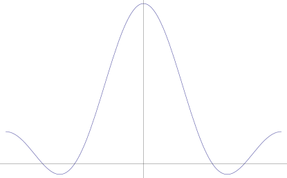
Figure 6.1: Shape of $Z_{-}\cos(\eta)+E\cos^{2}(\eta)$ in $[-\pi,\pi]$.

We construct our quasimodes to be concentrated near one of the minima. Let the intervals $\Delta_{o}^{+}$ and $\Delta_{i}^{+}$ be two open neighborhoods of the rightmost minima such that $\overline{\Delta_{i}^{+}}\subset\Delta_{o}^{+}$ and $\Delta_{o}^{+}$ is contained in the positive axis and is strictly separated from $0$. Fix $\chi_{+}\in C_{0}^{\infty}({\mathbb{R}})$ such that $\chi_{+}=1$ in $\Delta_{i}^{+}$ and $\chi_{+}=0$ in ${\mathbb{R}}\setminus\Delta_{o}^{+}$.

Lemma 6.14.

Let $P_{h}$ be as in (6.12) but with $V(x):=\frac{(x-x_{*})^{2}}{4}+W(x)$ and $W(x):=\sum_{m=m_{0}}^{\infty}a_{m}(x-x_{*})^{m}$ ($m_{0}>2$) entire of order $1$ and finite type. Define

$$\psi^{h}_{n}(x):=h^{-\frac{1}{4}}D_{n}\left(h^{-\frac{1}{2}}(x-x_{*})\right)\chi_{+}(x)=D^{h}_{n}(x-x_{*})\chi_{+}(x),$$

where $\chi_{+}$ is the characteristic function defined in the previous paragraph. Then $(\psi^{h}_{n}(x),E_{n}^{h})$ is an ${\cal O}\left(h^{3/2}\right)$-quasimode for $P_{h}$.

Proof. Applying the operator to $\psi^{h}_{n}$ we have

$$P_{h}\psi^{h}_{n}={} -h^{2}{\psi^{h}_{n}}^{\prime\prime}+\frac{(x-x_{*})^{2}}{4}\psi^{h}_{n}+W\;\psi^{h}_{n}$$

$$={} \left(-h^{2}{D^{h}_{n}}^{\prime\prime}+\frac{(x-x_{*})^{2}}{4}D^{h}_{n}+W\;D^{h}_{n}\right)\chi_{+}-h^{2}\left(2h^{-\frac{1}{2}}{D^{h}_{n}}^{\prime}\chi_{+}^{\prime}+D^{h}_{n}\chi^{\prime\prime}\right)$$

$$\overset{(\ref{eq-Phdefsinglemin})}{=} E^{h}_{n}\psi^{h}_{n}+W\;\psi^{h}_{n}-h^{2}\left(2h^{-\frac{1}{2}}{D^{h}_{n}}^{\prime}\chi_{+}^{\prime}+D^{h}_{n}\chi^{\prime\prime}\right).$$

For what concerns $W\;\psi^{h}_{n}$ we can apply Lemma 6.13, obtaining

$$\|W\cdot\psi^{h}_{n}\|={\cal O}\left(h^{\frac{m_{0}}{2}}\right).$$

We need now to take care of the last error term. For this last term the inequality

$$\left|h^{2}\left(2h^{-\frac{1}{2}}{D^{h}_{n}}^{\prime}\chi_{+}^{\prime}+D^{h}_{n}\chi^{\prime\prime}\right)\right|\leq hc_{1}e^{-\frac{c_{2}}{h}}$$

holds with proper $c_{1},c_{2}>0$ (that depend only on $n$ and $\chi_{+}$). Thus this term integrated on $[a,b]$ will give an error that can be bounded with any polynomial order of decay, in particular we can choose it to be

$$\left\|h^{2}\left(2h^{-\frac{1}{2}}{D^{h}_{n}}^{\prime}\chi_{+}^{\prime}+D^{h}_{n}\chi^{\prime\prime}\right)\right\|={\cal O}\left(h^{\frac{m_{0}}{2}}\right).\hfill$$

We need now to transform our equation into something like $V(x)$ in the previous theorem. We already know the two minima $\pm\eta_{*}$. If we expand $V(\eta):=Z_{-}\cos(\eta)+E\cos^{2}(\eta)$ in the neighborhood of those minima we obtain

$$V(x)=-\frac{Z_{-}^{2}}{4E}+E\left(1-\frac{Z_{-}^{2}}{4E^{2}}\right)(\eta\pm\eta_{*})^{2}+W(\eta\pm\eta_{*})$$ (6.15)

for a suitable entire $W$ with $m_{0}=3$ and of order $1$ and finite type.

To simplify a bit the notation let us call

$$A:=-\frac{Z_{-}^{2}}{4E}\;,\qquad B:=\sqrt{E\left(1-\frac{Z_{-}^{2}}{4E^{2}}\right)}.$$

We focus for the moment only the localisation near the rightmost minima, i.e. we choose $(\eta-\eta_{*})$. With the unitary transformation ${\mathcal{Z}}$ defined by change of variable

$$z(\eta):=\sqrt{2B}(\eta-\eta_{*}),$$

the eigenvalue equation (6.10) is transformed into

$$0=K_{z}\psi(z):=2B\left(-h^{2}\partial_{\eta}^{2}\psi(z)+\left(\widetilde{\mu}+\frac{z^{2}}{4}+\widetilde{W}(z)\right)\psi(z)\right),$$ (6.16)

where $\widetilde{\mu}=\frac{1}{2B}(-\mu+A)$ and $\widetilde{W}$ is entire with $m_{0}=3$ and of order $1$ and finite type. If in the spirit of the previous lemmas we define

$$\widetilde{\psi}^{h}_{n}(z):=D^{h}_{n}(z)\chi(z),\qquad\widetilde{\mu}_{n}^{h}:=A+2B\left(n+{\textstyle\frac{1}{2}}\right)h,$$

where $\chi(z)$ is the transformed of the cut-off localised in the neighborhood of $\eta_{*}$, then the couple $(\widetilde{\psi}^{h}_{n},\widetilde{\mu}_{n}^{h})$ is an ${\cal O}(h^{3/2})$-quasimode for $K_{z}$ and thus if

$$\psi^{h}_{n}(\eta):=\left({\mathcal{Z}}^{-1}\widetilde{\psi}^{h}_{n}{\mathcal{Z}}\right)(\eta),$$

the couple $(\psi^{h}_{n\pm},\widetilde{\mu}_{n}^{h})$ defines an ${\cal O}(h^{3/2})$-quasimode for $K_{\eta}$.

Exactly the same happens if we look near the other minimum, i.e. if we choose $(\eta+\eta_{*})$. In other words in the limit of $h\searrow 0$ the spectrum of $K_{\eta}$ consists of pairs $\mu_{n}^{-}(h)$, $\mu_{n}^{+}(h)$ with the same asymptotics $\widetilde{\mu}_{n}^{h}$ in the limit. We have proved the following.

Theorem 6.15.

Let $E>\frac{Z_{-}}{2}>0$. Define

$$\widetilde{\mu}_{n}^{h}:=-\frac{Z_{-}^{2}}{4E}+\sqrt{E\left(1-\frac{Z_{-}^{2}}{4E^{2}}\right)}\left(2n+1\right)h.$$ (6.17)

There exists an eigenvalue $\mu_{n}^{h}$ of $K_{\eta}$ and a constant $c$ such that $\left|\widetilde{\mu}_{n}^{h}-\mu_{n}^{h}\right|={\mathcal{O}}(h^{3/2})$. Moreover, the interval $\left[\widetilde{\mu}_{n}^{h}-2ch^{3/2},\;\widetilde{\mu}_{n}^{h}+2ch^{3/2}\right]$ contains at least two eigenvalues of $K_{\eta}$.

Remark 6.16.

It can be proved by standard methods involving the IMS formula [14, Chapter 3.1] and Agmon estimates [2] that the distance between the eigenvalues in each pair is of the order $\exp(-C/h)$ with $C\in(0,\infty)$. $\Diamond$

We can use this result in combination with (6.7).

Proposition 6.17.

The resonances in the set ${\mathcal{R}}_{n}\cap\{\Re E>\frac{Z_{-}}{2}>0\}$ (see (6.2)) are given asymptotically as $h\to 0$ by the solutions of the following equation

$$A_{n}(h,E,Z_{+},\mu^{+}_{m}(h,E))=0.$$ (6.18)

Neglecting the error terms, the resonances for $\Re E>\frac{Z_{-}}{2}>0$ are given by the solutions of

$$-E-Z_{+}-\textstyle{\frac{Z_{-}^{2}}{4E}+\sqrt{E-\frac{Z_{-}^{2}}{4E}}\left(2m+1\right)}h+ih(2n+1)\sqrt{\textstyle{\sqrt{E-\frac{Z_{-}^{2}}{4E}}\left(2m+1\right)h-\frac{Z_{-}^{2}}{4E}-\frac{Z_{+}}{2}}}=0.$$

Remark 6.18.

For $Z_{-}=0$ we recover (6.9) of the previous section. On the other hand, in Section 6.3 the approximation error is of order ${\cal O}(h^{2})$ instead of ${\cal O}(h^{3/2})$. $\Diamond$

For $0<E<\frac{Z_{-}}{2}$ the bottom of the potential is reached at $\pi$ and thus we have to expand the potential around this other point. It turns out that in this case the eigenvalues are approximated by

$$\widehat{\mu}_{n}^{h}:=E-Z_{-}+\sqrt{\textstyle{\frac{Z_{-}}{2}}-E}\left(2n+1\right)h.$$ (6.19)

Proposition 6.19.

The resonances in the set ${\mathcal{R}}_{n}\cap\{0<\Re E<\frac{Z_{-}}{2}\}$ (see (6.2)) are given asymptotically as $h\to 0$ by the solutions of the following equation

$$A_{n}(h,E,Z_{+},\widehat{\mu}^{+}_{m}(h,E))=0.$$

Remark 6.20.

This approach gives good results if we stay localised near the bottom of the potential: in this case we can find an approximation for the eigenvalue up to an order of any integer power of $h$.

The deficiency of this approach lies in the fact that we have no control on the relative error between $n$ and $h$. We need therefore to find a different approximation scheme that keeps track of the mutual relation between the parameters. $\Diamond$

6.5 High energy estimates

We consider the potential in the form $V(x)=E\cos^{2}(x)+Z_{-}\cos(x)$. Substituting this value in the formulae given in Theorem A.4 we have

$$\int_{-\pi}^{\pi}V(x)\,dx=E\pi\quad\mbox{and}\quad\int_{-\pi}^{\pi}V^{2}(x)\,dx=\frac{3E^{2}\pi}{4}+\pi Z_{-}^{2}$$

and thus the eigenvalues $\mu_{2m+1}$ and $\mu_{2m+2}$ can be represented as

$$\sqrt{\mu}=(m+1)h+\frac{E}{4(m+1)h}+\frac{Z_{-}^{2}-\frac{E^{2}}{4}}{16(m+1)^{3}h^{3}}+{\cal O}\left(\frac{1}{m^{5}h^{5}}\right)+o\left(\frac{1}{m^{3}h}\right).$$ (6.20)

Therefore we can estimate $\mu_{2m+1}$ and $\mu_{2m+2}$ with

$$\mu=(m+1)^{2}h^{2}+\frac{E}{2}+\left(Z_{-}^{2}+\frac{E^{2}}{4}\right)\frac{1}{8(m+1)^{2}h^{2}}+{\cal O}\left(\frac{1}{m^{4}h^{4}}\right)+o\left(\frac{1}{m^{2}}\right).$$ (6.21)

With this result, we can compute the resonances $E_{n,2m+1}$ and $E_{n,2m+2}$.

Proposition 6.21.

The resonances in the set ${\mathcal{R}}_{n}$ (see (6.2)) are given by the solutions of the following equation

$$A_{n}(h,E,Z_{+},\mu_{2m+1}(h,E))=0,$$ (6.22)

asymptotically as $h\to 0$ and $m\to\infty$ with $mh$ large.

More explicitly, for fixed $n$ and up to errors of orders

$$h^{\frac{3}{2}},\qquad(mh)^{-4}\quad\mbox{and}\quad m^{-2},$$

we can approximate the resonant energies as solutions of

$$-\frac{E}{2}-Z_{+}+(m+1)^{2}h^{2}+\frac{Z_{-}^{2}+\frac{E^{2}}{4}}{8(m+1)^{2}h^{2}}+i(2n+1)h\sqrt{\textstyle{(m+1)^{2}h^{2}+\frac{E-Z_{+}}{2}+\frac{Z_{-}^{2}+\frac{E^{2}}{4}}{8(m+1)^{2}h^{2}}}}=0.$$

Remark 6.22.

We cannot hide the term $(m+1)^{2}h^{2}$ inside the error term of order $h^{3/2}$ because we want to analyze the asymptotic behaviour for $m\geq C/h$ ($C\in(0,\infty)$) and that term is rather big compared with $h$. $\Diamond$

7 Numerical investigations

In the previous sections we have explicitly written three implicit equations to approximate the value of the resonances in terms of the atomic numbers $n$ and $m$ (and of course of the parameters $h$, $Z_{+}$ and $Z_{-}$). In this section we investigate the qualitative structure of the resonances using the approximations given by (6.18) and (6.22).

In view of Remarks 6.7 and 6.8 we know that at least for certain values of the charges $Z_{i}$ we are not describing all the resonances of the system. On the other hand the additional resonances should appear only for small $\Re(E)$. Therefore we are going to consider $\Re(E)$ big enough to be sure that we are analysing an energy region in which all the resonances should be generated by the classical closed hyperbolic trajectory between the centers.

In this case equation (6.8) implies that $\Re(\mu_{m})$ must be big and thus it is evident from (6.17), (6.19) and (6.21) that $m$ must be big. The quasimode approximation obtained in Section 6.3 and 6.4 is valid only for small values of $m$ and $h$, therefore these resonances are automatically excluded from the analysis.

Figure 7.11(a) and 7.11(b) show all the approximated resonances obtained from (6.18) setting $Z_{-}=0$. We plotted all the values including the one in regions of energies where we have no control on the error. In these pictures we can observe an interesting behaviour. In particular for big values of $m$ we recover the structure shown by the resonances approximated with (6.22): see Figure 7.22(a) and Figure 7.22(b).

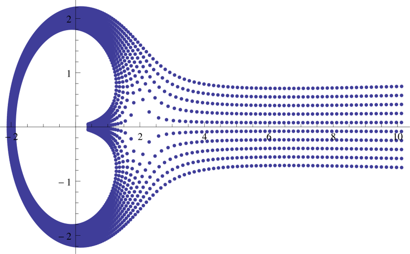
(a) Case $Z_{+}=2$.

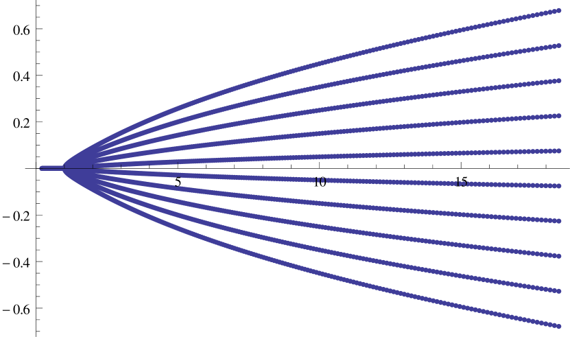
(b) Case $Z_{+}=-2$.

Figure 7.1: Solutions of (6.18) with $Z_{-}=0$, $h=0.01$, $n=0,\ldots,4$, $m=1,\dots,250$.

The physically interesting resonances are the ones close to the real axis, this because they can be measured in experiments. Thus to keep $\Im(E)$ as small as possible we will consider small values of $n$ (see (6.8)).

Remark 7.1.

Unless differently specified, in the plots we consider $n=0,1,2,3$ and $m\in\left\{\lceil C/h\rceil+k\mid k=0,1,2,\ldots,20\right\}$. The values of $Z_{+}$, $Z_{-}$, $h$ and $C$ will be specified in the title or in the caption of the plots. For practical reasons we plot the resonances in the plane $(\Re(E),-\Im(E))$. $\Diamond$

Equation (6.22) has two couples of solutions $(S_{+},L_{+})$ and $(S_{-},L_{-})$, specular w.r.t. the real axis. They correspond respectively to the resonances and the anti-resonances, i.e. the resonances defined inverting the roles of the incoming and outgoing waves $v_{\pm}$ in the construction of Section 4.3.

We restrict our analysis to the resonances $(S_{+},L_{+})$. The two sets $S_{+},L_{+}\in{\mathbb{C}}_{-}$ characterise two different energy regions, this meaning that the resonances in $S_{+}$ have relatively small real part if compared to the resonances in $L_{+}$ (see Figure 7.22(a) and Figure 7.22(b)).

(a) Resonances in $L_{+}$.

(b) Resonances in $S_{+}$.

Figure 7.2: Resonances for $h=0.05$ and $C=10$.

The structure that we find is extremely regular. The first question that arises is if we are really computing the resonances associated with energy values on the critical line ${\mathcal{L}}_{+}^{2}$, associated to the hyperbolic closed orbits described in [32, 49] and summarised in Section 2.3.

For each computed resonance $E_{n,m}$ we can use the approximation obtained in (6.21) to estimate the associated constant of motion $K_{n,m}$. We can thus superimpose the points $(\Re(E),\Re(K))$ to the bifurcation diagram and visualize how they are related. As shown in Figure 3(b), the energy parameters appear to lay exactly upon ${\mathcal{L}}_{+}^{2}$, giving a strong hint on the correctness of the result.

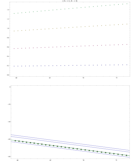
(a) $(Z_{+},Z_{-})=(2,4)$, $C=4$, $m=400,\ldots,430$.

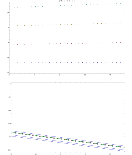
(b) $(Z_{+},Z_{-})=(-2,4)$, $C=7$, $m=700,\ldots,730$.

Figure 7.3: Comparison of the resonances in $L_{+}$ for $h=0.001$ (plot above) and their projection on the bifurcation diagram (plot below).

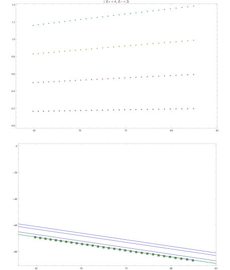
(c) $(Z_{+},Z_{-})=(4,2)$, $C=4$, $m=400,\ldots,430$.

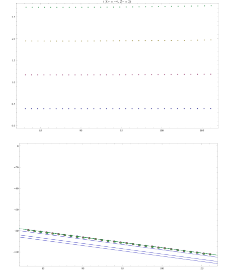
(d) $(Z_{+},Z_{-})=(-4,2)$, $C=7$, $m=700,\ldots,730$.

A related question regards the order of growth of the resonances $E_{n,m}$ in $n$ and $m$. For large energies there is only one bounded trajectory, which is closed and hyperbolic. In the corresponding case for pseudo-differential operators the real respectively imaginary parts of the resonances in the complex plane are known to be related to the action resp. Lyapunov spectrum of the the closed trajectory (see [19] for the physics perspective and [20] for a mathematical proof).
For a two-centers system it is known that the Lyapunov exponent of the bounded orbit of energy $E$ diverges like $\ell(E)=\sqrt{E}\ln(E)$ (see [32, Proposition 5.6]). As these closed trajectories collide with the two centers, where the Coulombic potential diverges, these results are not applicable. However it is reasonable to normalize the real and imaginary part of the resonances in $L_{+}$ (or $S_{+}$) dividing them by $\ell(\Re(E))$. In this way it is possible to investigate, at least qualitatively, the above prediction.

The numerics confirm the expected behaviour. It is evident from Figure 7.44(a) and 7.44(b) that the renormalised resonances look like distributed on a regular lattice of points with (almost perfectly) aligned and equispaced real and imaginary parts.

Notice moreover that the vertical spacing of the imaginary parts is $d={\cal O}(h)$ and the distance between the real axis and the resonances with smaller imaginary part is approximately $d/2$, as expected from the harmonic oscillator perturbation used to approximate the resonances.

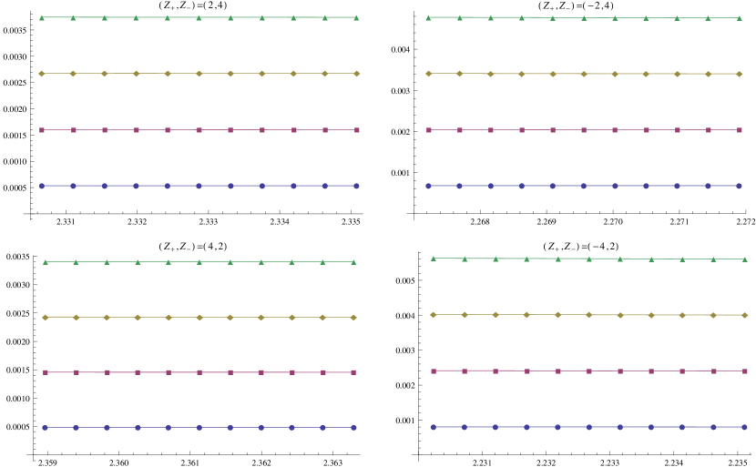
(a) Plot for for $E\in L_{+}$.

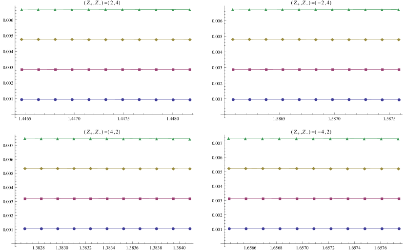
(b) Plot for $E\in S_{+}$.

Figure 7.4: Renormalised resonances $E/\ell(\Re(E))$ with parameters $h=0.001$, $C=9$ and $m=9000,\ldots,9010$.

8 The two-center problem in 3D and the $n$-center problem

In [48, Chapters 3 and 5] it is shown that the three-dimensional two-centers system is not essentially different from the planar one. In particular all the results obtained for the planar problem and presented in this paper can be carried almost identical.

However two major difficulties arises. There is a non-trivial effect coming from the angular momentum that makes the resonances set more complex and potentially more degenerate. And the numerical approximations that we get in the planar setting fail to hold due to the presence of singularities produced by the angular momentum.

Another important related problem is the study of resonances for the $n$-centers system. The classical model for $n\geq 3$ still presents hyperbolic bounded trajectories [32, 33]. In this case however they form a Cantor set in the phase space. Moreover the non-trapping condition fails to hold, thus in the quantum case one expects the resonances to be present and to be distributed in some complicated way. There are only few known examples presenting a similar structure that have been investigated rigorously (see [42] and [51]). They suggests that the resonances are present and their density near the real energy axis scales with a fractal power of $h$. The results obtained in this paper strongly support the idea that the resonances should be present and be strictly related with the underlying classical hyperbolic structure.

Anyhow for $n\geq 3$, mainly due to the lack of separability, the singularities of the potential have to be treated by semiclassical techniques, as in [11]. A lot of work and new ideas are required to properly extend results like [42, 51] to the $n$-center problem.

Appendix A Generalised Prüfer transformation in the semi-classical limit

The method for establishing estimates is based on a modification of the Prüfer variables described in [16, Chapter 4.1]. Consider a Sturm-Liouville differential equation on $[x_{1},x_{2}]$ of the form

$$(C(x)y^{\prime}(x))^{\prime}+D(x)y(x)=0$$ (A.1)

in which $C$ and $D$ are real-valued, not necessarily periodic, differentiable and with piecewise continuous derivatives. Suppose also that $C(x)$ and $D(x)$ are positive and define $R(x):=\sqrt{C(x)D(x)}$. If $y$ is a non-trivial real-valued solution of (A.1), we can write

$$R(x)y(x)=\rho(x)\sin(\theta(x)),\quad C(x)y^{\prime}(x)=\rho(x)\cos(\theta(x)),$$ (A.2)

where

$$\rho(x):=\sqrt{R^{2}(x)y^{2}(x)+C^{2}(x)y^{\prime 2}(x)}\quad\mbox{,}\quad\theta(x):=\arctan\left(\frac{R(x)y(x)}{C(x)y^{\prime}(x)}\right).$$

Up to now $\theta(x)$ is defined as a continuous function of $x$ only up to a multiple of $2\pi$. To solve this problem we select a point $a_{0}\in[x_{1},x_{2}]$ and we stipulate that $-\pi\leq\theta(a_{0})<\pi$. Moreover, if $y(a_{0})\geq 0$, we have by (A.1) that

$$0\leq\theta(a_{0})<\pi.$$ (A.3)

Lemma A.1.

With the above definitions

$$\theta^{\prime}(x)=\left(\frac{D(x)}{C(x)}\right)^{1/2}+\frac{1}{4}\frac{\left(C(x)D(x)\right)^{\prime}}{C(x)D(x)}\sin(2\theta(x)).$$ (A.4)

Let $a_{1}\in(a_{0},x_{2}]$. If $y(x)$ has $N$ zeroes in $(a_{0},a_{1}]$ and $y(a_{0})\geq 0$, then

$$N\pi\leq\theta(a_{1})<(N+1)\pi.$$ (A.5)

Proof.

The theorem is proved in [16, Chapter 4.1]. ∎

We want to apply (A.2) to equation (6.10). In particular we apply the transform to

$$h^{2}\big{(}p(x)y^{\prime}(x)\big{)}^{\prime}+\big{(}\mu-V_{1}(x)\big{)}y(x)=0$$ (A.6)

where $p$ and $V_{1}$ have period $2\pi$. Since we are concerned with the limit $\mu\rightarrow\infty$ (parametrically depending on $h$), we can consider $\mu$ large enough to have $\mu-V_{1}(x)>0$ in $[-\pi,\pi]$. In the new case (A.6) the two functions $\theta$ and $\rho$ depend on $\mu$ and $h$ as well as $x$, and we write $\theta_{h}(x,\mu)$. Then (A.4) becomes

$$\theta^{\prime}_{h}(x,\mu)=\frac{1}{h}\sqrt{\frac{\mu-V_{1}(x)}{p(x)}}+\frac{1}{4}\frac{\mu\,p^{\prime}(x)-(p(x)V_{1}(x))^{\prime}}{(\mu-V_{1}(x))p(x)}\sin(2\theta_{h}(x,\mu)).$$ (A.7)

A first consequence of (A.7) is that as $\mu\rightarrow\infty$

$$\theta^{\prime}_{h}(x,\mu)=\frac{\mu^{\frac{1}{2}}}{h}\sqrt{\frac{1-\widetilde{V}_{1}(x)}{p(x)}}+{\cal O}(1),$$ (A.8)

where $\widetilde{V}_{1}(x):=V_{1}(x)/\mu$. Moreover, if $y(x)$ has period $2\pi$ we have

$$\theta_{h}(\pi,\mu)-\theta_{h}(-\pi,\mu)=2k\pi$$ (A.9)

for an integer $k$.

Lemma A.2.

For $f\in L^{1}([-\pi,\pi])$ and $c\in{\mathbb{R}}\setminus\{0\}$ let $\theta_{h}(x,\mu)$ satisfy (A.7). Then

$$\int_{-\pi}^{\pi}f(x)\sin\left(c\,\theta_{h}(x,\mu)\right)dx\longrightarrow 0$$

as $\mu\rightarrow\infty$ (and/or $h\!\!\searrow\!\!0$). The same result holds with $\sin\left(c\,\theta_{h}(x,\mu)\right)$ replaced by $\cos\left(c\,\theta_{h}(x,\mu)\right)$.

Proof.

To keep the equations compact we drop the $\mu$ dependence of $\theta_{h}(x,\mu)$ in the rest of the proof. Fix any $\epsilon>0$. Let $g:[-\pi,\pi]\to{\mathbb{R}}$ be a continuously differentiable function such that

$$\int_{-\pi}^{\pi}\left|f(x)-g(x)\right|dx<\epsilon.$$

Then

$$\left|\int_{-\pi}^{\pi}f(x)\sin\left(c\,\theta_{h}(x)\right)dx\right|<\epsilon+\left|\int_{-\pi}^{\pi}g(x)\sin\left(c\,\theta_{h}(x)\right)dx\right|.$$ (A.10)

Define

$$G(x):=g(x)\sqrt{\frac{p(x)}{1-\widetilde{V}_{1}(x)}}.$$

Then by (A.8)

$$\int_{-\pi}^{\pi}g(x)\sin\left(c\,\theta_{h}(x)\right)\,dx=\frac{h}{\mu^{\frac{1}{2}}}\int_{-\pi}^{\pi}G(x)\sin\left(c\,\theta_{h}(x)\right)\theta^{\prime}_{h}(x)\,dx+{\cal O}\left(\frac{h}{\mu^{\frac{1}{2}}}\right)$$

$$=\frac{h}{c\,\mu^{\frac{1}{2}}}\Big{(}\left[G(x)\cos\left(c\,\theta_{h}(x)\right)\right]_{-\pi}^{\pi}-\int_{-\pi}^{\pi}G^{\prime}(x)\cos\left(c\,\theta_{h}(x)\right)dx\Big{)}+{\cal O}\left(\frac{h}{\mu^{\frac{1}{2}}}\right).$$

Hence

$$\left|\int_{-\pi}^{\pi}g(x)\sin\left(c\,\theta_{h}(x)\right)dx\right|\leq\frac{h}{\mu^{\frac{1}{2}}}K(g)<\epsilon$$

if $\mu$ is large enough, $K(g)$ being a number independent of $\mu$. The lemma follows by the genericity of $\epsilon$ and (A.10). ∎

For $\mu\to\infty$, the first term on the right hand side of (A.7) can be rewritten expanding the square root as

$$\textstyle\frac{1}{h}\sqrt{\frac{\mu-V_{1}(x)}{p(x)}}=\frac{\mu^{\frac{1}{2}}}{h\sqrt{p(x)}}\left(1-\frac{V_{1}(x)}{2\mu}+{\cal O}\left(\mu^{-2}\right)\right)=\frac{\mu^{\frac{1}{2}}}{h\,\sqrt{p(x)}}-\frac{V_{1}(x)}{2h\mu^{\frac{1}{2}}\,\sqrt{p(x)}}+{\cal O}\left(\frac{1}{h\mu^{\frac{3}{2}}}\right).$$

Then, in the case $p(x)=1$,

$$\theta^{\prime}_{h}(x,\mu)=\frac{1}{h}\sqrt{\mu-V_{1}(x)}-\frac{1}{4}\frac{V_{1}^{\prime}(x)}{\mu-V_{1}(x)}\sin(2\theta_{h}(x,\mu)),$$ (A.11)

and asymptotically as $\mu\to\infty$ the first term on the right hand side becomes

$$\frac{1}{h}\sqrt{\mu-V_{1}(x)}=\frac{\mu^{\frac{1}{2}}}{h}-\frac{V_{1}(x)}{2h\mu^{\frac{1}{2}}}+{\cal O}\left(\frac{1}{h\mu^{\frac{3}{2}}}\right).$$ (A.12)

Let $\mu_{n}$ ($n\in{\mathbb{N}}$) denote the eigenvalues of the Sturm-Liouville periodic problem (A.6) in ascending order (the potential being denoted by $V$ instead of $V_{1}$). By standard theory of Sturm-Liouville problems (see [16, Theorems 2.3.1 and 3.1.2]) the spectrum is pure point, and the $\mu_{n}$ are at most doubly degenerate and accumulate at infinity.

Theorem A.3.

Let $p(x)=1$. Then as $m\to\infty$, $\mu_{2m+1}$ and $\mu_{2m+2}$ both satisfy

$$\sqrt{\mu}=(m+1)h+\frac{\int_{-\pi}^{\pi}V(x)\,dx}{4\pi(m+1)h}+o\left(\frac{1}{mh}\right).$$

Proof.

Fix an $\epsilon>0$. Let $V_{1}$ be a continuously differentiable function with period $2\pi$ such that

$$V_{1}(x)\geq V(x)\quad\mbox{and}\quad\int_{-\pi}^{\pi}V_{1}(x)\,dx\leq\epsilon+\int_{-\pi}^{\pi}V(x)\,dx.$$ (A.13)

Let $\mu_{1,n}$ denote the eigenvalue in the periodic problem associated with $V_{1}(x)$ (and with $p(x)=1$) and $\psi_{1,n}$ its eigenfunction. Then by [16, Theorem 2.2.2] and the first eq. in (A.13) we have

$$\mu_{1,n}\geq\mu_{n}.$$

We can assume that $\psi_{1,n}(-\pi)\geq 0$ and we apply the modified Prüfer transformation to $y(x)=\psi_{1,2m+1}(x)$ with $a_{0}=-\pi$ in (A.3). Now, from (A.3) and (A.9) we have

$$2k\pi\leq\theta(\pi,\mu_{1,2m+1})<(2k+1)\pi$$

for some integer $k$. From the standard theory of Sturm-Liouville problems (see aforementioned reference) we know that $\psi_{1,2m+1}$ has $2(m+1)$ zeroes in $(-\pi,\pi]$, hence by (A.5) with $a_{1}=\pi$ we have $2k=2(m+1)$ and thus

$$\theta_{h}(\pi,\mu_{1,2m+1})-\theta(-\pi,\mu_{1,2m+1})=2(m+1)\pi.$$ (A.14)

Integrating (A.11) with $\mu=\mu_{1,2m+1}$ over $[-\pi,\pi]$ we obtain

$$2(m+1)\pi=\int_{-\pi}^{\pi}\frac{1}{h}\sqrt{\mu-V_{1}(x)}\,dx-\frac{1}{4}\int_{-\pi}^{\pi}\frac{V_{1}^{\prime}(x)}{\mu-V_{1}(x)}\sin(2\theta_{h}(x,\mu))\,dx.$$ (A.15)

By Lemma A.2 the rightmost term is $o(\mu^{-1})$ as $m\to\infty$ (becoming $o(h/m^{2})$ in (A.16) and thus being suppressed from the equation). For the first integral on the right we can use the binomial expansion as in (A.12). Thus (A.15) gives

$$2(m+1)\pi=\frac{\mu^{\frac{1}{2}}}{h}2\pi-\frac{\int_{-\pi}^{\pi}V_{1}(x)\,dx}{2h\mu^{\frac{1}{2}}}+{\cal O}\left(\frac{1}{h\mu^{\frac{3}{2}}}\right)$$

that is

$$\mu-(m+1)h\sqrt{\mu}-\frac{1}{4\pi}\int_{-\pi}^{\pi}V_{1}(x)\,dx+{\cal O}\left(\frac{1}{\mu}\right)=0.$$

Solving for $\mu$ one gets

$$\sqrt{\mu}=\frac{1}{2}\left((m+1)h+\sqrt{(m+1)^{2}h^{2}+\frac{1}{\pi}\int_{-\pi}^{\pi}V_{1}(x)\,dx+{\cal O}(\mu^{-1})}\right).$$

Extracting $(m+1)h$ and using once more the binomial expansion one gets

$$\sqrt{\mu_{2m+1}}=(m+1)h+\frac{\int_{-\pi}^{\pi}V_{1}(x)\,dx}{4\pi(m+1)h}+{\cal O}\left(\frac{1}{m^{2}h^{2}}\right).$$ (A.16)

Hence by (A.13) and by the fact that $\epsilon$ is arbitrarily small

$$\sqrt{\mu_{2m+1}}\leq(m+1)h+\frac{\int_{-\pi}^{\pi}V(x)\,dx}{4\pi(m+1)h}+o\left(\frac{1}{mh}\right).$$

The opposite inequality can be proved in the same way. The result for $\mu_{2m+1}$ holds in the same form using the fact that its eigenfunction must have $2(m+1)$ zeroes. ∎

So far we have not used any differentiability-related property of $V$. Using the differentiability, we can make the previous estimate much more precise for $m$ large.

Theorem A.4.

Let $p(x)=1$, let $r\in{\mathbb{N}}$, and let $\frac{d^{r}}{dx^{r}}V(x)$ exist and be piecewise continuous. Then $\mu_{2m+1}$ and $\mu_{2m+2}$ both satisfy

$$\sqrt{\mu}=(m+1)h+\sum_{k=1}^{r+1}\frac{A_{k}}{(m+1)^{k}h^{k}}+{\cal O}\left(\frac{1}{m^{r+2}h^{r+2}}\right)+o\left(\frac{1}{m^{r+1}h^{r-2}}\right)$$

where the $A_{k}$ are independent of $m$ and involve $q(x)$ and its derivatives up to order $r-1$. In particular,

$$A_{1}=\frac{1}{4\pi}\int_{-\pi}^{\pi}V(x)\,dx\quad\mbox{,}\quad A_{2}=0\quad\mbox{and}\quad A_{3}=\frac{1}{16\pi}\int_{-\pi}^{\pi}V^{2}(x)\,dx-A_{1}^{2}.$$ (A.17)

Proof.

We consider $V_{1}=V$ in (A.11). Then $\mu_{1,n}=\mu_{n}$ and the case $r=1$ corresponds simply to (A.16). To deal with $r\geq 2$ we reconsider (A.15), which is now

$$2(m+1)\pi=\int_{-\pi}^{\pi}\frac{1}{h}\sqrt{\mu-V(x)}\,dx-\frac{1}{4}\int_{-\pi}^{\pi}\frac{V^{\prime}(x)}{\mu-V(x)}\sin(2\theta_{h}(x,\mu))\,dx$$ (A.18)

and $\mu$ is $\mu_{2m+1}$ or $\mu_{2m+2}$. By (A.11), with $V_{1}=V$, the second integral on the right in (A.18) is

$$\int_{\pi}^{\pi}\frac{hV^{\prime}(x)}{(\mu-V(x))^{\frac{3}{2}}} \left(\theta^{\prime}_{h}(x,\mu)+\frac{1}{4}\frac{V_{1}^{\prime}(x)}{\mu-V_{1}(x)}\sin(2\theta_{h}(x,\mu))\right)\sin(2\theta_{h}(x,\mu))\,dx$$

$$={} \frac{h}{2}\int_{-\pi}^{\pi}\left(\frac{d}{dx}\frac{V^{\prime}(x)}{(\mu-V(x))^{\frac{3}{2}}}\right)\cos(2\theta_{h}(x,\mu))\,dx$$ (A.19)

$$+\frac{h}{8}\int_{-\pi}^{\pi}\frac{V^{\prime 2}(x)}{(\mu-V(x))^{\frac{5}{2}}}\,dx-\frac{h}{8}\int_{-\pi}^{\pi}\frac{V^{\prime 2}(x)}{(\mu-V(x))^{\frac{5}{2}}}\cos(4\theta_{h}(x,\mu))\,dx$$

after integrating by parts. The first term on the right here is $o\left(h\mu^{-\frac{3}{2}}\right)$ by Lemma A.2, the last is $o\left(h\mu^{-\frac{5}{2}}\right)$ for the same reason and the central one is ${\cal O}\left(h\mu^{-\frac{5}{2}}\right)$. This, together with the binomial expansion of $\sqrt{\mu-V(x)}$ in the first term on the right of (A.18) gives

$$2(m+1)\pi=\frac{\mu^{\frac{1}{2}}}{h}2\pi-\frac{\int_{-\pi}^{\pi}V(x)\,dx}{2h\mu^{\frac{1}{2}}}-\frac{\int_{-\pi}^{\pi}V^{2}(x)\,dx}{8h\mu^{\frac{3}{2}}}+{\cal O}\left(\frac{1}{h\mu^{\frac{5}{2}}}\right)+o\left(\frac{h}{\mu^{\frac{3}{2}}}\right)$$ (A.20)

To solve (A.20) for $\mu^{\frac{1}{2}}$ in terms of $m$, we write it as

$$\mu^{\frac{1}{2}}=M+\mu^{-\frac{1}{2}}A_{1}+\mu^{-\frac{3}{2}}(A_{3}-A_{1}^{2})+{\cal O}\left(\frac{1}{m^{5}h^{5}}\right)+o\left(\frac{1}{m^{3}h}\right)$$ (A.21)

where $M=h(m+1)$. Then, taking the reciprocals we obtain

$$\mu^{-\frac{1}{2}} =M^{-1}\left(1-\mu^{-\frac{1}{2}}A_{1}M^{-1}+{\cal O}(h^{-4}m^{-4})\right)=M^{-1}-M^{-3}A_{1}+{\cal O}(h^{-5}m^{-5}).$$ (A.22)

And thus,

$$\mu^{-\frac{3}{2}}=M^{-3}+{\cal O}(h^{-5}m^{-5}).$$ (A.23)

Substituting (A.22) and (A.23) into (A.21) give the result for $r=2$.

To deal with $r=3$, we introduce $\theta^{\prime}(x,\mu)$ into the integrals in (A.19) involving $\cos(2\theta_{h}(x,\mu))$ and $\cos(4\theta_{h}(x,\mu))$, exactly as we did for (A.18). Then, if $\frac{d^{3}}{dx^{3}}V(x)$ exists and is piecewise continuous, we can integrate by parts as before. The binomial expansions of $\frac{1}{h}\sqrt{\mu-V(x)}$ and $(\mu-V(x))^{-\frac{3}{2}}$ extend (A.20) to $o\left(h^{2}\mu^{-\frac{5}{2}}\right)+{\cal O}\left(h^{-1}\mu^{-\frac{7}{2}}\right)$ giving the result for $r=3$. The process can be continued as long as $q(x)$ is sufficiently differentiable for the integration by parts to be carried out, and the theorem is proved. ∎

Remark A.5.

We can intend Theorem A.4 as the result of analytic perturbation theory of

$$h^{2}(p(x)y^{\prime}(x))^{\prime}+y(x)=0$$

(derived from (A.6)) in terms of the parameter $V_{1}(x)/\mu$. As a consequence we get $A_{2k}=0$ for all $k\in{\mathbb{N}}$. $\Diamond$

References

- [1] Ralph Abraham and Jerrold E. Marsden. Foundations of Mechanics. Benjamin Cummings, 1978.
- [2] Shmuel Agmon. Lectures on exponential decay of solutions of second-order elliptic equations: bounds on eigenfunctions of -body Schrödinger operators, volume 29 of Mathematical Notes. Princeton University Press, Princeton, NJ, 1982.
- [3] Shmuel Agmon and Markus Klein. Analyticity properties in scattering and spectral theory for Schrödinger operators with long-range radial potentials. Duke Math. J., 68(2):337–399, 1992.
- [4] Joachim Asch and Andreas Knauf. Quantum transport on KAM tori. Comm. Math. Phys., 205(1):113–128, 1999.
- [5] W. G. Baber and H. R. Hassé. The Two Centre Problem in Wave Mechanics. Proceedings of the Cambridge Philosophical Society, 31:564, 1935.
- [6] Ph. Briet, J.-M. Combes, and P. Duclos. On the location of resonances for Schrödinger operators in the semiclassical limit. I. Resonances free domains. J. Math. Anal. Appl., 126(1):90–99, 1987.
- [7] Ph. Briet, J.-M. Combes, and P. Duclos. On the location of resonances for Schrödinger operators in the semiclassical limit. II. Barrier top resonances. Communications in Partial Differential Equations, 12(2):201–222, 1987.
- [8] Ph. Briet, J.-M. Combes, and P. Duclos. Erratum for: on the location of resonance for Schrödinger operations in the semiclassical limit. II. Barrier top resonances. Communications in Partial Differential Equations, 13(3):377–381, 1988.
- [9] B. M. Brown, D. K. R. McCormack, W. D. Evans, and M. Plum. On the spectrum of second-order differential operators with complex coefficients. R. Soc. Lond. Proc. Ser. A Math. Phys. Eng. Sci., 455(1984):1235–1257, 1999.
- [10] W. Byers-Brown and E. Steiner. On the electronic energy of a one-electron diatomic molecule near the united atom. Journal of Chemical Physics, 44:3934–3940, 1966.
- [11] François Castella, Thierry Jecko, and Andreas Knauf. Semiclassical resolvent estimates for Schrödinger operators with Coulomb singularities. Ann. Henri Poincaré, 9(4):775–815, 2008.
- [12] Earl A. Coddington and Norman Levinson. Theory of ordinary differential equations. McGraw-Hill Book Company, Inc., New York-Toronto-London, 1955.
- [13] John B. Conway. Functions of one complex variable, volume 11 of Graduate Texts in Mathematics. Springer-Verlag, New York, second edition, 1978.
- [14] H. L. Cycon, R. G. Froese, W. Kirsch, and B. Simon. Schrödinger operators with application to quantum mechanics and global geometry. Texts and Monographs in Physics. Springer-Verlag, Berlin, 1987.
- [15] J. Cízek, R.J. Damburg, S. Graffi, Grecchi V., E.M. Harrell, II, J.G. Harris, S. Nakai, J. Paldus, R.K. Propin, and H.J. Silverstone. expansion for : Calculation of exponentially small terms and asymptotics. Phys Rev A Gen Phys, 33:12–54, 1986.
- [16] M. S. P. Eastham. The Spectral Theory of Periodic Differential Equations. Scottish Academic Press, Edimburgh, 1975.
- [17] M. S. P. Eastham. The asymptotic solution of linear differential systems, volume 4 of London Mathematical Society Monographs. New Series. The Clarendon Press Oxford University Press, New York, 1989. Applications of the Levinson theorem, Oxford Science Publications.
- [18] Arthur Erdélyi, Wilhelm Magnus, Fritz Oberhettinger, and Francesco G. Tricomi. Higher transcendental functions. Vol. III. McGraw-Hill Book Company, Inc., New York-Toronto-London, 1955. Based, in part, on notes left by Harry Bateman.
- [19] P. Gaspard, D. Alonso, and I. Burghardt. New Ways of Understanding Semiclassical Quantization. Advances in Chemical Physics, 90:105–364, 1995.
- [20] C. Gérard and J. Sjöstrand. Semiclassical resonances generated by a closed trajectory of hyperbolic type. Comm. Math. Phys., 108(3):391–421, 1987.
- [21] S. Graffi, V. Grecchi, E. M. Harrell, II, and H. J. Silverstone. The expansion for : analyticity, summability, and asymptotics. Ann. Physics, 165(2):441–483, 1985.
- [22] P. Thornton Greenland and Walter Greiner. Two centre continuum Coulomb wavefunctions in the entire complex plane. Theoretical Chemistry Accounts: Theory, Computation, and Modeling (Theoretica Chimica Acta), 42:273–291, 1976.
- [23] Gisèle Hadinger, M Aubert-Frécon, and Gerold Hadinger. Continuum wavefunctions for one-electron two-centre molecular ions from the Killingbeck-Miller method. Journal of Physics B: Atomic, Molecular and Optical Physics, 29(14):2951, 1996.
- [24] E. Harrell and B. Simon. The mathematical theory of resonances whose widths are exponentially small. Duke Math. J., 47(4):845–902, 1980.
- [25] Evans M. Harrell, Noel Corngold, and Barry Simon. The mathematical theory of resonances whose widths are exponentially small. II. J. Math. Anal. Appl., 99(2):447–457, 1984.
- [26] Bernard Helffer and André Martinez. Comparaison entre les diverses notions de résonances. Helv. Phys. Acta, 60(8):992–1003, 1987.
- [27] P. D. Hislop and I. M. Sigal. Introduction to spectral theory, volume 113 of Applied Mathematical Sciences. Springer-Verlag, New York, 1996. With applications to Schrödinger operators.
- [28] C. G. J. Jacobi. C.G.J. Jacobi’s Vorlesungen über Dynamik. G. Reimer, Berlin, 1884.
- [29] Th. Jecko, M. Klein, and X.P. Wang. Existence and Born-Oppenheimer asymptotics of the total scattering cross-section in ion-atom collisions. “Long time behaviour of classical and quantum systems”, proceedings of the Bologna AP-TEX international conference, 1999. edited by A. Martinez and S. Graffi.
- [30] Tosio Kato. Perturbation theory for linear operators. Classics in Mathematics. Springer-Verlag, Berlin, 1995. Reprint of the 1980 edition.
- [31] M. Klaus. On for small internuclear separation. Journal of Physics A: Mathematical and General, 16:2709–2720, 1983.
- [32] Marcus Klein and Andreas Knauf. Classical Planar Scattering by Coulombic Potentials. Number v. 13 in Lecture notes in physics: Monographs. Springer, 1992.
- [33] Andreas Knauf. The -centre problem of celestial mechanics for large energies. J. Eur. Math. Soc. (JEMS), 4(1):1–114, 2002.
- [34] Vladimir F. Lazutkin. KAM theory and semiclassical approximations to eigenfunctions, volume 24 of Ergebnisse der Mathematik und ihrer Grenzgebiete (3) [Results in Mathematics and Related Areas (3)]. Springer-Verlag, Berlin, 1993. With an addendum by A. I. Shnirel′man.
- [35] E. W. Leaver. Solutions to a generalized spheroidal wave equation: Teukolsky’s equations in general relativity, and the two-center problem in molecular quantum mechanics. J. Math. Phys., 27(5):1238–1265, 1986.
- [36] J. W. Liu. Analytical solutions to the generalized spheroidal wave equation and the Green’s function of one-electron diatomic molecules. Journal of Mathematical Physics, 33(12):4026–4036, 1992.
- [37] Wilhelm Magnus and Stanley Winkler. Hill’s equation. Dover Publications Inc., New York, 1979. Corrected reprint of the 1966 edition.
- [38] A. Martinez. Resonance free domains for non globally analytic potentials. Ann. Henri Poincaré, 3(4):739–756, 2002.
- [39] A. Martinez. Erratum to: “Resonance free domains for non globally analytic potentials”. Ann. Henri Poincaré, 8(7):1425–1431, 2007.
- [40] Josef Meixner, Friedrich W. Schäfke, and Gerhard Wolf. Mathieu functions and spheroidal functions and their mathematical foundations, volume 837 of Lecture Notes in Mathematics. Springer-Verlag, Berlin, 1980. Further studies.
- [41] Josef Meixner and Friedrich Wilhelm Schäfke. Mathieusche Funktionen und Sphäroidfunktionen mit Anwendungen auf physikalische und technische Probleme. Die Grundlehren der mathematischen Wissenschaften in Einzeldarstellungen mit besonderer Berücksichtigung der Anwendungsgebiete, Band LXXI. Springer-Verlag, Berlin, 1954.
- [42] Stéphane Nonnenmacher and Maciej Zworski. Fractal Weyl laws in discrete models of chaotic scattering. J. Phys. A, 38(49):10683–10702, 2005.
- [43] Wolfgang Pauli. Über das Modell des Wasserstoffmolekülions. Annalen der Physik, 373(11):177–240, 1922.
- [44] Michael Reed and Barry Simon. Methods of modern mathematical physics. II. Fourier analysis, self-adjointness. Academic Press, New York, 1975.
- [45] Michael Reed and Barry Simon. Methods of modern mathematical physics. IV. Analysis of operators. Academic Press, New York, 1978.
- [46] Michael Reed and Barry Simon. Methods of modern mathematical physics. I. Academic Press Inc., New York, second edition, 1980. Functional analysis.
- [47] Tony C. Scott, Monique Aubert-Frécon, and Johannes Grotendorst. New approach for the electronic energies of the hydrogen molecular ion. Chemical Physics, 324(2–3):323 – 338, 2006.
- [48] M. Seri. Resonances in the Two Centers Coulomb System, www.opus.ub.uni-erlangen.de/opus/volltexte/2012/3546. PhD thesis, Friedrich-Alexander-University Erlangen-Nuremberg, 09.2012.
- [49] M. Seri. The Problem of Two Fixed Centers: Bifurcation Diagram for Positive Energies. J. Math. Phys., 56:012902, 2015.
- [50] Johannes Sjöstrand. Semiclassical resonances generated by nondegenerate critical points. In Pseudodifferential operators (Oberwolfach, 1986), volume 1256 of Lecture Notes in Math., pages 402–429. Springer, Berlin, 1987.
- [51] Johannes Sjöstrand and Maciej Zworski. Fractal upper bounds on the density of semiclassical resonances. Duke Math. J., 137(3):381–459, 2007.
- [52] Sergei Yu. Slavyanov and Wolfgang Lay. Special functions. Oxford Mathematical Monographs. Oxford University Press, Oxford, 2000. A unified theory based on singularities, With a foreword by Alfred Seeger, Oxford Science Publications.
- [53] M. P. Strand and W. P. Reinhardt. Semiclassical quantization of the low lying electronic states of . J. Chem. Phys., 70:3812–3827, April 1979.
- [54] M. J. O. Strutt. Reelle Eigenwerte verallgemeinerter Hillscher Eigenwertaufgaben 2. Ordnung. Math. Z., 49:593–643, 1944.
- [55] Gerald Teschl. Ordinary Differential Equations and Dynamical Systems. Lecture Notes. University of Vienna, 2000.
- [56] F. G. Tricomi. Integral equations. Dover Publications Inc., New York, 1985. Reprint of the 1957 original.
- [57] Hans Volkmer. Quadratic growth of convergence radii for eigenvalues of two-parameter Sturm-Liouville equations. J. Differential Equations, 128(1):327–345, 1996.
- [58] Hans Volkmer. On the growth of convergence radii for the eigenvalues of the Mathieu equation. Math. Nachr., 192:239–253, 1998.
- [59] Hans Volkmer. On Riemann surfaces of analytic eigenvalue functions. Complex Var. Theory Appl., 49(3):169–182, 2004.
- [60] Holger Waalkens, Holger R. Dullin, and Peter H. Richter. The problem of two fixed centers: bifurcations, actions, monodromy. Phys. D, 196(3-4):265–310, 2004.
- [61] Joachim Weidmann. Spectral theory of ordinary differential operators, volume 1258 of Lecture Notes in Mathematics. Springer-Verlag, Berlin, 1987.
- [62] Maciej Zworski. Resonances in physics and geometry. Notices Amer. Math. Soc., 46(3):319–328, 1999.