The Problem of Two Fixed Centers: Bifurcation Diagram for Positive Energies

Abstract

We give a comprehensive analysis of the Euler-Jacobi problem of motion in the field of two fixed centers with arbitrary relative strength and for positive values of the energy. These systems represent nontrivial examples of integrable dynamics and are analysed from the point of view of the energy-momentum mapping from the phase space to the space of the integration constants. In this setting we describe the structure of the scattering trajectories in phase space and derive an explicit description of the bifurcation diagram, i.e. the set of critical value of the energy-momentum map.

Keywords: Two-center problem; Integrable systems; Bifurcation diagram.

Mathematics Subject Classification: 37J20, 37D05

1 Introduction

The study of two-centers Coulombic systems, both from a classical and quantum point of view, is distributed along the last three centuries, starting from pioneering works of Euler in 1760, Jacobi [Jac84] in 1884 and Pauli [Pau22] from a quantum mechanical point of view in 1922.

Indeed, the models described by these systems are important both for macroscopic and microscopic systems: in celestial mechanics they model the motion of a test particle attracted by two fixed stars, and in molecular physics they represent the simplest models for one-electron diatomic molecules (e.g. the ions ${\rm H}_{2}^{+}$ and ${\rm HHe}^{2+}$) and appear as the first term in the Born-Oppenheimer approximation of molecules.

Among the central features of this class of models is their integrability and the separability in elliptical coordinates. This makes possible to introduce a number of significant reductions in the study and therefore makes te model very suitable as a test field for a number of questions.

Despite the age and the many properties of the problem, the research around it goes up to the present days [WDR04, Kna02, SAFG06] and there are present many challenges that have to be addressed.

This work is a necessary step to prepare the foundations for the study of the quantum resonances of the planar quantum mechanical two-centers Coulomb system in the semi-classical limit [SKDEJ]. Additionally the planar restriction of the two-centers problem arise naturally in the analysis of the three-dimensional system one as an essential prototypical building block [Ser12].

A comprehensive analysis for the negative energies picture has been given by Waalkens, Dullin and Richter [WDR04]. The classical scattering was studied and described by Knauf and Klein [KK92, Kna02]. The contribution of this work is the completion of the phase space picture and of the bifurcation diagram for the two-centers systems with arbitrary relative strengths in the case of positive energies (see Theorem 3.5 and its corollaries). For positive energies we are in a scattering situation and the orbits foliate the space into families of diffeomorphic cylinders, the bifurcation diagrams let us describe the different families of trajectories and their properties.

Quantum resonances are a key notion of quantum physics: roughly speaking they are scattering states (i.e. states of the essential spectrum) that for long time behave like bound states (i.e. eigenfunctions). They are usually defined as poles of a meromorphic function, but there is not really a unique way to study and define them [Zwo99]. On the other hand, it is known that their many definitions coincide in some settings [HM87] and that their existence is related to the presence of some classical orbits “trapped” by the potential.

The importance of this work in the setting of quantum resonances lies in the strong connection between these and the structure of the underlying classical system. In fact it has been proven that there are resonances generated by classical bounded trajectories around local minima of the potential [HS96] and that there are resonances generated by closed hyperbolic trajectories or by non-degenerate maxima of the potential [BCD87b, BCD88, Sjö87, GS87]. The main difference being in their asymptotic distance from the real axis in terms of the semiclassical parameter $h$.

Even the presence or absence of the resonances is strictly related to the classical picture. In fact it is possible to use some classical estimates, called non-trapping conditions, to prove the existence of resonance free regions (see for example [BCD87a, Mar02, Mar07]).

The failure of the non-trapping condition for the two-centers problem was already known in the literature [CJK08] as well as the presence of a close hyperbolic trajectory for positive energies [KK92]. With the present analysis we are able to explicitly identify the energies associated with this hyperbolic trajectory and to find a positive measure of positive energies associated to families of bounded trajectories. Their presence makes the present models a very good candidate for the study of quantum resonances in presence of singular potential [SKDEJ, Ser12].

Notation. In this article $0\not\in{\mathbb{N}}$, ${\mathbb{R}}^{*}:={\mathbb{R}}\setminus\{0\}$ and ${\mathbb{R}}_{+}:=(0,\infty)$.

2 The classical problem of two Coulomb centers

We consider the classical Hamiltonian function on the cotangent bundle $T^{*}Q_{2}$ of $Q_{2}:={\mathbb{R}}^{2}\setminus\{s_{1},s_{2}\}$ relative to the $2$-center potential given by:

$$H:T^{*}Q_{2}\to{\mathbb{R}}\quad\mbox{,}\quad H(p,q):=\frac{|p|^{2}}{2}+\frac{-Z_{1}}{|q-s_{1}|}+\frac{-Z_{2}}{|q-s_{2}|}.$$ (2.1)

This describes the motion of a test particle in the field of two bodies of relative strengths $Z_{i}\in{\mathbb{R}}^{*}={\mathbb{R}}\setminus\{0\}$, fixed at positions $s_{1}\neq s_{2}\in{\mathbb{R}}^{2}$. By the unitary realisation $Uf(x):=|\det A|^{-1/2}f(Ax+b)$ of an affinity of ${\mathbb{R}}^{2}$ we assume that the two centers are at $s_{1}:=a:=\left(\begin{smallmatrix}1\\ 0\end{smallmatrix}\right)$ and $s_{2}:=-a$.

2.1 Elliptic coordinates

The restriction to the rectangle $M:={\mathbb{R}}_{+}\times(-\pi,\pi)$ of the map

$$G:{\mathbb{R}}^{2}\to{\mathbb{R}}^{2}\quad\mbox{,}\quad\left(\begin{smallmatrix}\xi\\ \eta\end{smallmatrix}\right)\mapsto\left(\begin{smallmatrix}\cosh(\xi)\cos(\eta)\\ \sinh(\xi)\sin(\eta)\end{smallmatrix}\right)$$ (2.2)

defines a $C^{\infty}$ diffeomorphism

$$G:M\to G(M)$$ (2.3)

whose image $G(M)={\mathbb{R}}^{2}\setminus({\mathbb{R}}\times\{0\})$ is dense in ${\mathbb{R}}^{2}$. Moreover it defines a change of coordinates from $q\in{\mathbb{R}}^{2}$ to $(\xi,\eta)\in M$. These new coordinates are called elliptic coordinates.

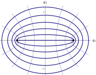
Figure 2.1: Elliptic coordinates.

Remarks 2.1.

1. In the $(q_{1},q_{2})$-plane the curves $\xi=c$ are ellipses with foci at $\pm a$, while the curves $\eta=c$ are confocal half hyperbolas, see Figure 2.1.

2. The Jacobian determinant of $G$ equals

   $$F(\xi,\eta):=\det(DG(\xi,\eta))=\sinh^{2}(\xi)+\sin^{2}(\eta)=\cosh^{2}(\xi)-\cos^{2}(\eta).$$ (2.4)

   Thus the coordinate change (2.2) is degenerate at the points $(\xi,\eta)\in\{0\}\times\{0,\pm\pi\}$ in $\overline{M}$. For $\xi=0$ the $\eta$ coordinate parametrizes the $q_{1}$-axis interval between the two centers. For $\eta=0$ ($\eta=\pm\pi$) the $\xi$ coordinate parametrizes the positive (negative) $q_{1}$-axis with $|q_{1}|>1$. $\Diamond$

2.2 Hamiltonian setting

Lemma 2.2.

Using $G$ defined in (2.3), and $Z_{\pm}:=Z_{2}\pm Z_{1}$, $H$ is transformed by the elliptic coordinates into

$$H\circ{(G^{-1})^{*}}(p_{\xi},p_{\eta},\xi,\eta)=\frac{1}{F(\xi,\eta)}\big{(}H_{1}(p_{\xi},\xi)+H_{2}(p_{\eta},\eta)\big{)}$$ (2.5)

where $(G^{-1})^{*}:T^{*}M\to T^{*}Q_{2}$ is the cotangential lift of $G^{-1}$, and

$$H_{1}(p_{\xi},\xi):=\frac{p_{\xi}^{2}}{2}-Z_{+}\cosh(\xi)\quad\mbox{,}\quad H_{2}(p_{\eta},\eta):=\frac{p_{\eta}^{2}}{2}+Z_{-}\cos(\eta).$$ (2.6)

There are two functionally independent constants of motion $H$ and $L:=H_{1}-\cosh^{2}(\xi)H$ with values $E$ and $K$ respectively.

Proof.

Although the lemma is well-known (see, e.g., Thirring [Thi88], Sect. 4.3), we indicate its proof, in order to introduce some notation: If we apply to $H$ the canonical point transformation induced by the elliptic coordinates (2.3), the potential is transformed as

$$V\circ G(\xi,\eta)=-\frac{Z_{1}}{|q-a|}-\frac{Z_{2}}{|q+a|}={-\frac{Z_{+}\cosh(\xi)-Z_{-}\cos(\eta)}{F(\xi,\eta)}},$$ (2.7)

and the momenta $p=(p_{1},p_{2})$ are transformed according to

$$\left(\begin{smallmatrix}p_{1}\\ p_{2}\end{smallmatrix}\right)=(DG(\xi,\eta)^{-1})^{t}\left(\begin{smallmatrix}p_{\xi}\\ p_{\eta}\end{smallmatrix}\right).$$

From $(DG(\xi,\eta)^{-1})(DG(\xi,\eta)^{-1})^{t}=(DG(\xi,\eta)^{t}DG(\xi,\eta))^{-1}$ and

$$(DG(\xi,\eta)^{t}DG(\xi,\eta))=\left(\begin{smallmatrix}F(\xi,\eta)&0\\ 0&F(\xi,\eta)\end{smallmatrix}\right)$$

we get that the Hamiltonian is transformed into (2.5). ∎

Given an initial condition $x_{0}\in T^{*}Q_{2}$ we set $E:=H(x_{0})$.

Equation (2.5) can be again separated [Kna11, Lemma 10.38] moving to the extended phase space and using a new time parameter $s$ defined by

$$\frac{dt}{ds}=F(\xi,\eta).$$

One obtains the new Hamiltonian

$$\widetilde{H}:=F(\xi,\eta)(H-E)=H_{\xi}+H_{\eta}$$

where

$$H_{\xi}(p_{\xi},\xi):=H_{1}-\cosh^{2}(\xi)E\quad\mbox{and}\quad H_{\eta}(p_{\eta},\eta):=H_{2}+\cos^{2}(\eta)E.$$ (2.8)

On the submanifold $\widetilde{H}^{-1}(0)$, $\widetilde{H}$ describes the time evolution of $H^{-1}(E)$ up to a time reparametrisation. Therefore we have a second constant of motion other than $H$:

$$L:=H_{1}-\cosh^{2}(\xi)E=-\left(H_{2}+\cos^{2}(\eta)E\right).$$ (2.9)

Setting $K:=H_{\xi}(x_{0})=-H_{\eta}(x_{0})$ we have two constants of motion $H$ and $H_{\xi}$ whose values are denoted respectively $E$ and $K$. Notice that these functions are generally independent in the following sense. Being real analytic functions, the subset of phase space where independence is violated, is of Lebesgue measure zero. ∎

Remarks 2.3.

1. By the previous proof, we can restrict our attention to the phase space $T^{*}Q_{2}$ with Hamiltonian

   $$\widehat{H}(p_{\xi},p_{\eta},\xi,\eta)=H_{\xi}(p_{\xi},\xi)+H_{\eta}(p_{\eta},\eta),$$

   where the $H_{\xi}$ and $H_{\eta}$ are defined in (2.8) and have the form

   $$H_{\xi}(p_{\xi},\xi):=\frac{p_{\xi}^{2}}{2}+V_{\xi}(\xi),\qquad H_{\eta}(p_{\eta},\eta):=\frac{p_{\eta}^{2}}{2}+V_{\eta}(\eta).$$ (2.10)

   Here $V_{\xi}$ and $V_{\eta}$ are defined by

   $$V_{\xi}(\xi):=-Z_{+}\cosh(\xi)-E\cosh^{2}(\xi)\quad\mbox{,}\quad V_{\eta}(\eta):=Z_{-}\cos(\eta)+E\cos^{2}(\eta).$$ (2.11)

2. Notice that the trajectories may cross the $q_{1}$-axis (where the prolate elliptic coordinate are singular) and even collide with the two centers at $\pm a=(\pm 1,0)$. There are some different ways to regularise the motion both in the planar and spatial cases (and with an arbitrary number of centers), we refer the reader to [Kna02, Chapter 4-5], [KK92, Chapter 3] and [Kna11, Remark 11.24] for more details and references. $\Diamond$

3 Bifurcation diagrams

Taken together, the constants of motion define a vector valued function on the phase space of a Hamiltonian. We can study the structure of the preimages of this function (its level sets), in particular their topology. In the simplest case the level sets are mutually diffeomorphic manifolds.

Definition 3.1.

(see [AM78, Section 4.5]) Given two manifolds $M,N$, $f\in C^{\infty}(M,N)$ is called locally trivial at $y_{0}\in N$ if there exists a neighbourhood $V\subseteq N$ of $y_{0}$ such that $f^{-1}(y)$ is a smooth submanifold of $M$ for all $y\in V$ and there there is a map $g\in C^{\infty}(f^{-1}(V),f^{-1}(y_{0}))$ such that $f\times g:f^{-1}(V)\to V\times f^{-1}(y_{0})$ is a diffeomorphism.

The bifurcation set of $f$ is the set

$${\mathcal{B}}(f):=\{y_{0}\in N\mid f\mbox{ is not locally trivial at }y_{0}\}.$$

Notice that if $f$ is locally trivial, the restriction $g{\mathbin{\upharpoonright}}\raise-2.15277pt\hbox{$\scriptstyle f^{-1}(y)$}:f^{-1}(y)\to f^{-1}(y_{0})$ is a diffeomorphism for every $y\in V$.

Remark 3.2.

The critical points of $f$ lie in ${\mathcal{B}}(f)$ (see [AM78, Prop. 4.5.1]), but the converse is true only in the case $f$ is proper (i.e. it has compact preimages). $\Diamond$

Define the function on the phase space as follows (omitting a projection in the second component)

$${\mathcal{F}}:=\left(\begin{smallmatrix}H\\ H_{\xi}\circ G^{*}\end{smallmatrix}\right):T^{*}Q_{2}\to{\mathbb{R}}^{2}.$$ (3.1)

In what follows we characterise the bifurcation set ${\mathcal{B}}({\mathcal{F}})$.

3.1 Bifurcations for planar motions

We have already discussed the regularisability of the problem in Remark 2.3.2. In what follows we proceed similarly as [WDR04] but we consider the energy range $E\geq 0$.

It will be computationally useful to introduce a new coordinate change. The restriction to $M^{2}:=(1,\infty)\times(-1,1)$ of the map

$$\left(\begin{smallmatrix}x\\ y\end{smallmatrix}\right)\in\overline{M^{2}}\mapsto\left(\begin{smallmatrix}\operatorname{arccosh}(x)\\ \arccos(y)\end{smallmatrix}\right)\in{\mathbb{R}}^{2}$$

defines a $C^{\infty}$ diffeomorphism

$$G^{2}:M^{2}\to G^{2}(M^{2})$$ (3.2)

with image $G^{2}(M^{2})={\mathbb{R}}_{+}\times(0,\pi)\subsetneq M$. Therefore it defines a change of coordinates from $(\xi,\eta)\in{\mathbb{R}}_{+}\times(0,\pi)$ to $(x,y)\in M^{2}$.

Lemma 3.3.

The diffeomorphism defined in (3.2) induces a symplectomorphism $\widehat{G}^{2}:T^{*}({\mathbb{R}}_{+}\times(0,\pi))\to T^{*}M^{2}.$

Proof. It is enough to choose the generating function

$$S_{2}(\xi,\eta,p_{x},p_{y}):=\big{(}\cosh(\xi),\cos(\eta)\big{)}\left(\begin{smallmatrix}p_{x}\\ p_{y}\end{smallmatrix}\right).$$

It induces a canonical transformation

$$\widehat{G}^{2}:(p_{\xi},p_{\eta},\xi,\eta)\mapsto(p_{x},p_{y},x,y)$$

where

$$\left(\begin{smallmatrix}x\\ y\end{smallmatrix}\right)=\left(\begin{smallmatrix}\frac{\partial S_{2}}{\partial p_{x}}\\ \frac{\partial S_{2}}{\partial p_{y}}\end{smallmatrix}\right)=\left(\begin{smallmatrix}\cosh(\xi)\\ \cos(\eta)\end{smallmatrix}\right),\;\left(\begin{smallmatrix}p_{\xi}\\ p_{\eta}\end{smallmatrix}\right)=\left(\begin{smallmatrix}\frac{\partial S_{2}}{\partial\xi}\\ \frac{\partial S_{2}}{\partial\eta}\end{smallmatrix}\right)=\left(\begin{smallmatrix}\sinh(\xi)p_{x}\\ \sin(\eta)p_{y}\end{smallmatrix}\right)\hfill$$

To cover the $(q_{1},q_{2})$-plane of the configuration space $Q_{2}={\mathbb{R}}^{2}\setminus\{\pm a\}$ we need two half strips $[1,\infty)\times[-1,1]$ (i.e. one for each sign of $q_{2}$). Alternatively we can take the strip

$${\left(\begin{smallmatrix}\xi\\ \eta\end{smallmatrix}\right)\in\widetilde{Q}_{2}:=}{\mathbb{R}}\times[-\pi,\pi]$$

as the modified configuration space: For the map $\left(\begin{smallmatrix}\xi\\ \eta\end{smallmatrix}\right)\mapsto\left(\begin{smallmatrix}\cosh(\xi)\\ \cos(\eta)\end{smallmatrix}\right)$ it is a two-sheeted cover with branch points at the foci. The two sheets are related by the involution $I:(\xi,\eta)\mapsto(-\xi,-\eta)$ leaving the cartesian coordinates $(q_{1},q_{2})$ unchanged. The symplectic lift of $I$ to the phase space $T^{*}\widetilde{Q}_{2}$ equals

$$\widehat{I}:(p_{\xi},p_{\eta},\xi,\eta)\mapsto(-p_{\xi},-p_{\eta},-\xi,-\eta).$$

Then $T^{*}Q_{2}$ is obtained from $T^{*}\widetilde{Q}_{2}$ by factorisation with respect to ${\widehat{I}}$.

Remark 3.4.

An analysis of the extrema of $V_{\xi}$ and $V_{\eta}$ implies that the image ${\mathcal{R}}$ of $(H,H_{\xi})$ in ${\mathbb{R}}^{2}$ is bounded by the following curves. From $K=H_{\xi}\geq V_{\xi}$ we have $K\geq K_{+}(E)$ with

$$K_{+}(E):=\begin{cases}-\infty,&E>0\\ -(Z_{+}+E),&E\leq\min\left(-\frac{Z_{+}}{2},0\right)\\ \frac{Z_{+}^{2}}{4E},&0\geq E>\min\left(-\frac{Z_{+}}{2},0\right)\end{cases}$$ (3.2)

and from $-K=H_{\eta}\geq V_{\eta}$ we have $K\leq K_{-}(E)$ with

$$K_{-}(E):=\begin{cases}Z_{-}-E,&E\leq\frac{Z_{-}}{2}\\ \frac{Z_{-}^{2}}{4E},&E>\frac{Z_{-}}{2}\end{cases}.$$ (3.3)

The main objects of our analysis are transformed by the symplectomorphism defined in Theorem 3.3 as follows

$$\begin{array}[]{lclcl}F(\xi,\eta)&\mapsto&\hat{F}(x,y)&:=&x^{2}-y^{2},\\ V_{\xi}(\xi)&\mapsto&V_{x}(x)&:=&-Z_{+}x-Ex^{2},\\ V_{\eta}(\eta)&\mapsto&V_{y}(y)&:=&Z_{-}y+Ey^{2},\\ H_{\xi}(p_{\xi},\xi)&\mapsto&H_{x}(p_{x},x)&:=&\frac{(x^{2}-1)p_{x}^{2}}{2}+V_{x}(x),\\ H_{\eta}(p_{\eta},\eta)&\mapsto&H_{y}(p_{y},y)&:=&\frac{(1-y^{2})p_{y}^{2}}{2}+V_{y}(y).\end{array}$$ (3.4)

For the rest of the analysis we proceed with these transformed equations (3.4) keeping always in mind their relation with the $(\xi,\eta)$ variables.

Theorem 3.5.

Let $(Z_{1},Z_{2})\in{\mathbb{R}}^{*}\times{\mathbb{R}}^{*}$, then the bifurcation set of (3.1) equals

$${\mathcal{B}}\left({\mathcal{F}}\right){\upharpoonright}_{E\geq 0}=\left\{(E,K)\in{\mathcal{L}}\mid E\geq 0\text{ and }K_{+}(E)\leq K\leq K_{-}(E)\right\}.$$

Here ${\mathcal{L}}:={\mathcal{L}}_{0}\cup{\mathcal{L}}_{-}^{1}\cup{\mathcal{L}}_{-}^{2}\cup{\mathcal{L}}_{-}^{3}\cup{\mathcal{L}}_{+}^{2}\cup{\mathcal{L}}_{+}^{3}{\subset{\mathbb{R}}^{2}}$ with

$$\begin{array}[]{lcl}{\mathcal{L}}_{0}:=\{E=0\},&&{\mathcal{L}}_{-}^{1}:=\{K=Z_{-}-E\},\\ {\mathcal{L}}_{+}^{2}:=\{K=-Z_{+}-E\},&&{\mathcal{L}}_{-}^{2}:=\{K=-Z_{-}-E\},\\ {\mathcal{L}}_{+}^{3}:=\{4EK=Z_{+}^{2}\},&&{\mathcal{L}}_{-}^{3}:=\{4EK=Z_{-}^{2}\},\end{array}$$ (3.5)

and $K_{+}$ and $K_{-}$ are defined by (3.2) and (3.3).

Proof.

The fact that $K_{+}(E)\leq K\leq K_{-}(E)$ is a consequence of Remark 3.4.

$\{E=0\}$ is the threshold between compact and non compact energy surfaces. So by Definition 3.1 it belongs to the bifurcation set ${\mathcal{B}}\left({\mathcal{F}}\right)$.

By definition, the critical points of ${\mathcal{F}}$ are in ${\mathcal{B}}\left({\mathcal{F}}\right){\upharpoonright}_{E\geq 0}$. To compute them we can take advantage of the simple form of the level set equation in the $(x,y)$ coordinates. To cover the plane we need to consider two half strips (see Remark 2.1.1). We start assuming to cover the upper half plane. We can rewrite the level set equation

$${\mathcal{F}}(p_{x},p_{y},x,y)=\left(\begin{smallmatrix}H(p_{x},p_{y},x,y)\\ H_{x}(p_{x},x)\end{smallmatrix}\right)=\left(\begin{smallmatrix}E\\ K\end{smallmatrix}\right)$$

in the form

$$\left(\!\begin{array}[]{l}f_{1}(p_{y},y)\\ f_{2}(p_{x},x)\end{array}\!\right):=\left(\!\begin{array}[]{l}K+\frac{(1-y^{2})p_{y}^{2}}{2}+Z_{-}y+Ey^{2}\\ K-\frac{(x^{2}-1)p_{x}^{2}}{2}+Z_{+}x+Ex^{2}\end{array}\!\right)=\left(\!\begin{array}[]{l}0\\ 0\end{array}\!\right)$$ (3.6)

and use of this last representation to compute the critical points.

We look for values of $(p_{x},p_{y},x,y)$ such that

$$D\left(\begin{smallmatrix}f_{1}(p_{y},y)\\ f_{2}(p_{x},x)\end{smallmatrix}\right)=\left(\begin{smallmatrix}-(x^{2}-1)p_{x}&0&-xp_{x}^{2}+Z_{+}+2Ex&0\\ 0&(1-y^{2})p_{y}&0&-yp_{y}^{2}+2Ey+Z_{-}\end{smallmatrix}\right)$$

has rank smaller than $2$. Then, using $(x,y)\in[1,\infty)\times[-1,1]$, it a simple exercise to check that the critical points are given by the values

1. $(p_{x},\pm\sqrt{Z_{-}+2E},x,1)$ and $(p_{x},\pm\sqrt{Z_{-}-2E},x,-1)$,

2. $(p_{x},0,x,-Z_{-}/2E)$,

3. $(\pm\sqrt{Z_{+}+2E},p_{y},1,y)$,

4. $(0,p_{y},-Z_{+}/2E,y)$.

Substituting these values in the equations (3.6), one obtains the following curves in the $(E,K)$ plane

1. $K\pm Z_{-}+E=0$, thus ${\mathcal{L}}_{-}^{1,2}$ is in ${\mathcal{B}}\left({\mathcal{F}}\right)$,

2. $K-\frac{Z_{-}^{2}}{4E}=0$, thus ${\mathcal{L}}_{-}^{3}$ is in ${\mathcal{B}}\left({\mathcal{F}}\right)$,

3. $K+Z_{+}+E=0$, thus ${\mathcal{L}}_{+}^{2}$ is in ${\mathcal{B}}\left({\mathcal{F}}\right)$,

4. $K-\frac{Z_{+}^{2}}{4E}=0$, thus ${\mathcal{L}}_{+}^{3}$ is in ${\mathcal{B}}\left({\mathcal{F}}\right)$.

For what concerns the lower half plane covered by points $(x,y)$, it is enough to notice that its phase space equals the image of the one considered under the inversion $(p_{x},p_{y},x,y)\mapsto(p_{x},-p_{y},x,-y)$. Therefore it reduces to the analysis that we already performed.

We want to show that for all energy parameters $(E,K)$ in a connected component of ${\mathcal{R}}\setminus{\mathcal{B}}({\mathcal{F}})$ of the image ${\mathcal{R}}$ of ${\mathcal{F}}$, the energy levels ${\mathcal{F}}^{-1}(E,K)$ are diffeomorphic. We start by discussing a special example.

Let $(Z_{+},Z_{-})=(0,2)$. Let $(E_{0},K_{0})$ be in the interior of the region bounded by ${\mathcal{L}}_{-}^{1}$ and $K_{-}(E)$ (see Figure 3.1, bottom left plot). We will show in Section 3.3 that all the trajectories in configuration space with energy $(E_{0},K_{0})$ must cross a segment $S_{0}$ strictly contained in the segment joining the two centers (see Figure 3.4, plot 5 and 6 counted from the left). Since $(E_{0},K_{0})\not\in{\mathcal{L}}$ the crossing must be transversal. Therefore by the linearisability of the vector field we can define a Poincaré section $S_{0}$, such that every trajectory is uniquely identified by its crossing point (see [Kna11, Satz 3.46 and Definition 7.16]).

Let $(E_{1},K_{1})$ be another point in the interior of the region containing $(E_{0},K_{0})$. As before there is a segment $S_{1}$ strictly contained in the segment joining the two centers that is crossed transversally by all the trajectories (with energy $(E_{1},K_{1})$). Given $(E_{1},K_{1})$ we can define the Poincaré section $S_{1}$ and every point on the level set is identified by its crossing point and its time, thus the level set is diffeomorphic to ${\mathbb{R}}\times S_{1}$.

Clearly, $S_{0}$ and $S_{1}$ are diffeomorphic and thus the level sets of $(E_{0},K_{0})$ and $(E_{1},K_{1})$ are diffeomorphic. By the generality of $(E_{0},K_{0})$ and $(E_{1},K_{1})$ all the points in the interior of the region bounded by ${\mathcal{L}}_{-}^{1}$ and $K_{-}(E)$ have diffeomorphic level sets.

We consider another example, again $(Z_{+},Z_{-})=(0,2)$. Let $(E_{0},K_{0})$ be in the interior of the region of $\{E>0\}$ bounded by ${\mathcal{L}}_{+}^{2}$, ${\mathcal{L}}_{-}^{1}$ (see Figure 3.1, bottom left plot). We continue to refer to Section 3.3 when we show that for such $(E,K)$ all the trajectories in configuration space must cross a line segment $L_{0}$ strictly contained in the $q_{1}$-axis with $q_{1}<-1$ (see Figure 2.1 and the first plot from the right in Figure 3.4).

As in the previous example the trajectories must cross $L_{0}$ transversally and we can reduce the phase space to the Poincaré section $L_{0}$. If $(E_{1},K_{1})$ is another point in the same region we can reiterate the procedure to find a Poincaré section $L_{1}$ that is diffeomorphic to $L_{0}$. And thus all the points in the region have diffeomorphic level sets.

The argument sketched above can be reproduced in each connected component of ${\mathcal{R}}\setminus{\mathcal{B}}({\mathcal{F}})$ choosing a proper transversal section. How to make the choice will be clear in the next three sections, where we characterise the motion in configuration space for the energy parameters in each region. ∎

Remarks 3.6.

1. Differently from ${\mathcal{L}}_{0}=\{E=0\}$, the line $\{K=0\}$ is in the bifurcation set only in the symmetric case $Z_{-}=0$. In this case, in fact, it corresponds to the boundary $K_{-}(E)$ of the Hill’s region.

   Of course there may be points $\{K=0\}$ in the bifurcation set for $Z_{-}\neq 0$, but these are just the points in which curves in ${\mathcal{L}}$ cross $\{K=0\}$ transversally (see Figures 3.5 and 3.6).

2. The characterisation of the bifurcation set given in Theorem 3.5 is redundant. Namely some of the curves ${\mathcal{L}}_{*}^{*}$ restricted to the values of $(K,E)$ in the Hill’s region could be empty for some values of $Z_{1}$ and $Z_{2}$.

   For example, being $K\leq K_{-}(E)$, we can immediately see that the curve ${\mathcal{L}}_{+}^{3}$ will be in the bifurcation diagram for positive $E$ only when $Z_{+}<0$ and $|Z_{+}|<Z_{-}$. $\Diamond$

In what follows we will describe more precisely the structure of the bifurcation sets and of the trajectories in configuration space in relation to the values assumed by $Z_{+}$ and $Z_{-}$.

The momenta $(p_{x},p_{y})$ at given $(E,K)$ are given in general by

$$p_{x}^{2}=\frac{2(x^{2}-1)(Ex^{2}+Z_{+}x+K)}{(x^{2}-1)^{2}},\quad p_{y}^{2}=\frac{-2(1-y^{2})(Ey^{2}+Z_{-}y+K)}{(1-y^{2})^{2}}.$$ (3.7)

The Hill’s region is identified by the values of $E$ and $K$ that admit non-negative squared momenta. The denominators in (3.7) being always positive, we can discuss them and identify the possible motion types in terms of the zeros of the numerators, that is, the polynomials

$$P_{\pm}(s):=2(s^{2}-1)(Es^{2}+Z_{\pm}s+K).$$ (3.8)

Here $s\in\{x,y\}$ and the understanding is that we choose “$+$” for $s=x$ and “$-$” for $s=y$. The factor $(s^{2}-1)$ is introduced to provide the correct signs and for computational convenience. The momenta can be simply obtained via $(x^{2}-1)p_{x}=\pm\sqrt{P_{+}(x)}$ and $(1-y^{2})p_{y}=\pm\sqrt{P_{-}(y)}$. The roots of $P_{+}(x)$ and $P_{-}(y)$ are respectively

$$x_{1,2} =\pm 1,\qquad\textstyle x_{3,4}=-\frac{Z_{+}}{2E}\pm\sqrt{\frac{Z_{+}^{2}}{4E^{2}}-\frac{K}{E}},$$ (3.9)

$$y_{1,2} =\pm 1,\qquad\textstyle y_{3,4}=-\frac{Z_{-}}{2E}\pm\sqrt{\frac{Z_{-}^{2}}{4E^{2}}-\frac{K}{E}},$$

with the convention that the smaller index corresponds to the solution with negative sign. In both variables, the polynomials have two fixed roots at $\pm 1$ and two movable roots which depend on the constants of motion. Being $x\in[1,\infty)$, we are going to consider only roots in this region.

Figure 3.1: Examples of bifurcation diagrams for the considered planar cases, the shaded regions identify the complement of the Hill’s region, the red dashed curves are $K_{+}$ and $K_{-}$. The green line ${\mathcal{L}}_{+}^{2}$ parametrised by $K_{0}(E)=-(Z_{+}+E)$ corresponds to the closed orbit wandering between the two centers and having coordinate $x=1$. The box on the right shows the shape of the potential $V$ on the $q_{1}$-axis in the different cases.

The discriminant of $P_{\pm}$ is proportional to

$${\rm discr}(P_{\pm})=(Z_{\pm}^{2}-4EK)(E+K-Z_{\pm})^{2}(E+K+Z_{\pm})^{2}.$$ (3.10)

Double roots appear when ${\rm discr}(P_{\pm})$ vanishes. For each couple $(Z_{+},Z_{-})$ this gives six curves in the $(K,E)$-plane, three for the $x$ variable and three for the $y$. These are the curves ${\mathcal{L}}_{+}^{1}:=\{K=Z_{+}-E\}$ and ${\mathcal{L}}_{-}^{1}$, ${\mathcal{L}}_{\pm}^{2,3}$ defined by (3.5).

Remark 3.7.

The zeroes of the discriminant $P_{\pm}$ (3.10) correspond to the double roots of $(Es^{2}+Z_{\pm}s+K)$ and the points in which these roots reach the fixed roots $\pm 1$, i.e. the $q_{1}$-line. The positivity of $P_{\pm}$ and the positions of its roots, as we will see, characterise the trajectories in configuration space.

The curve ${\mathcal{L}}_{+}^{1}$ appearing in the discriminant depends from the fact that we considered $x\in{\mathbb{R}}$. As such it will have no correspondence in the bifurcation set or in the description of the possible motions. $\Diamond$

As a first step we consider the cases in which $Z_{-}=0$ or $Z_{+}=0$. In these cases the $(K,E)$-plane is divided by the curves ${\mathcal{L}}_{\pm}^{1,2,3}$ into different regions. We will label these regions using roman numbers with a subscript chosen between $>$, $<$ and $0$ indicating if $Z_{+}>0$, $Z_{+}<0$ or $Z_{+}=0$ respectively. In Figure 3.1 are shown representative bifurcation diagrams for these three cases with the corresponding enumeration of the regions.

3.2 Motion for $Z_{-}=0$

The case $Z_{-}=0$ corresponds to two attracting (or repelling) centers with the same relative strength. We have the following corollary of Theorem 3.5.

Corollary 3.8.

Let $Z_{-}=0$ and $Z_{+}\in{\mathbb{R}}^{*}$. With the notation of (3.5) we have

$${\mathcal{B}}({\mathcal{F}}){\mathbin{\upharpoonright}}\raise-2.15277pt\hbox{$\scriptstyle E\geq 0$}=\left\{(E,K)\in{\mathcal{L}}_{0}\cup{\mathcal{L}}_{-}^{1}\cup{\mathcal{L}}_{+}^{2}\mid E\geq 0\mbox{ and }K_{+}(E)\leq K\leq 0\right\}.$$

Proof.

In (2.1) we assumed $Z_{1},Z_{2}\neq 0$, therefore $Z_{-}=0$ implies $Z_{+}\neq 0$.

$K$ cannot be positive because $K_{-}(E)=0$ for $E\geq 0$. By ${\mathcal{L}}_{-}^{1}={\mathcal{L}}_{-}^{2}$ and ${\mathcal{L}}_{-}^{3}={\mathcal{L}}_{0}$, it is redundant to add both in the definition of the bifurcation diagram. The fact that ${\mathcal{L}}_{+}^{3}$ is not in the bifurcation set follows from Remark 3.6.2. Then the claim follows directly from Theorem 3.5. ∎

Consider the bifurcation diagram for $(Z_{+},Z_{-})=(\pm 2,0)$ appearing in Figure 3.1. It is possible to describe the qualitative structure of the motion in configuration space for energy parameters in the different regions by studying the dynamic of the roots (3.9) with respect to a walk in the bifurcation diagram. By this we mean fixing a value of $E$ big enough and varying $K$ to move through the regular regions $I_{>,<}$, $II_{>,<}$, $III_{>,<}$ and to cross the bifurcation lines.

A qualitative representation of how the motion changes with respect to the energy parameters is shown in Figure 3.2 for $Z_{+}=2$ and in Figure 3.3 for $Z_{+}=-2$. This can be schematically explained through the behaviour of the roots (3.9) as follows.

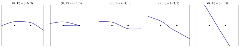
Figure 3.2: Example of possible trajectories in the case $Z_{+}=2$, $Z_{-}=0$ for $E=3$ and growing values of $K$ (from left to right) chosen in the different regions of the bifurcation diagram.

• Roots of the polynomial $P_{-}(y)$.

  • For energies in the regions $I_{>,<}$ and $II_{>}$ of the bifurcation diagrams, the polynomial $P_{-}(y)$ is non-negative for every value of $y\in[-1,1]$ and $|y_{3,4}|>1$. Thus for energy parameters in these regions, the particle is allowed travel in configuration space everywhere in a region around the centers.

  • Line ${\mathcal{L}}_{-}^{1}$ characterises the values $(E,K)$ such that the two groups of roots of $P_{-}(y)$ merge: $y_{3}=y_{1}=-1$ and $y_{4}=y_{2}=1$.

  • In the regions $II_{<}$ and $III_{>,<}$, $|y_{3,4}|<1$ and the $P_{-}(y)$ is not negative only if $y\in[y_{3},y_{4}]$. This means that the motion in configuration space can cross the axis through the two centers only passing through the segment between the centers.

• Roots of the polynomial $P_{+}(x)$.

  • Notice that $x_{1}$ and $x_{3}$ are always smaller than $1$, thus they do not belong to the domain of definition $[1,\infty)$ for $x$.

  • In the regions $I_{>,<}$ and $II_{<}$, the root $x_{4}>1$ and $P_{+}(x)$ is non negative only if $x\in[x_{4},\infty)$. Therefore in configuration space, the particle cannot reach the line joining the two centers.

  • For $(E,V)\in{\mathcal{L}}^{2}_{+}$, we have the collision of the solutions $x_{4}=x_{2}=1$ and in configuration space the particle can reach the line between the centers.

  • On the right of ${\mathcal{L}}^{2}_{+}$, in the regions $II_{>}$ and $III_{>/<}$, the root $x_{4}<1$ and $P_{+}(x)$ is non-negative for $x\in[1,\infty)$. In other words the particle can cross the line in configuration space connecting the centers.

We can now understand the peculiarity of the lines in the bifurcation set.

• For values of the parameters on the singular line ${\mathcal{L}}_{-}^{1}$ we can identify two special trajectories in configuration space. In these, the particle lies in the positive (negative) $q_{1}$-axis with $|q_{1}|>1$, possibly bouncing against the singularity and being reflected back.

• For $(E,V)$ on ${\mathcal{L}}^{2}_{+}$ we can find the unique periodic orbit of the regularised classical two-centers problem, see [Kna02]. It is the hyperbolic trajectory of a particle bouncing between the centers. Counting from left to right, the second plot of Figure 3.2 and the fourth plot of Figure 3.3 show the trajectory of a particle on the stable manifold of this special orbit.

• For $K=0$ ($E>0$) only one trajectory is possible: the vertical trajectory moving on the line $y=0$.

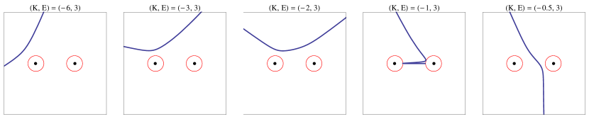
Figure 3.3: Example of possible trajectories in the case $Z_{+}=-2$, $Z_{-}=0$ for $E=3$ and growing values of $K$ (from left to right) chosen in the different regions of the bifurcation diagram. The red line corresponds to the energy level of the plotted trajectory.

Remark 3.9.

Notice that the ordering of the singular curves reflects the main difference between the cases $Z_{+}>0$ and $Z_{+}<0$. In the first case (corresponding to the attracting potential) the particle is able to travel arbitrarily near to the centers. In the case $Z_{+}<0$ the centers $\pm a$ have a positive distance from the Hill’s region. $\Diamond$

3.3 Motion for $Z_{+}=0$

Corollary 3.10.

Let $Z_{+}=0$ and $Z_{-}>0$. With the notation of (3.5) we have

$${\mathcal{B}}({\mathcal{F}}){\mathbin{\upharpoonright}}\raise-2.15277pt\hbox{$\scriptstyle E\geq 0$}=\Big{\{}(E,K)\in{}{\mathcal{L}}_{0}\cup{\mathcal{L}}_{-}^{1}\cup{\mathcal{L}}_{-}^{2}\cup{\mathcal{L}}_{-}^{3}\cup{\mathcal{L}}_{+}^{2}\mid E\geq 0\mbox{ and }K_{+}(E)\leq K\leq K_{-}(E)\Big{\}}.$$

Proof.

In (2.1) we assumed $Z_{1},Z_{2}\neq 0$, therefore $Z_{+}=0$ implies $Z_{-}\neq 0$.

We have ${\mathcal{L}}_{+}^{3}={\mathcal{L}}_{0}$. The claim follows directly from Theorem 3.5. ∎

As in the previous section we give a qualitative explanation of the possible motions in configuration space through the behaviour of the roots (3.9). A visual support is provided by Figure 3.4.

• Roots of the polynomial $P_{-}(y)$.

  • For $(E,V)$ in $I_{0}$, the polynomial $P_{-}(y)$ is not negative for any $y\in[-1,1]$. Thus in configuration space the particle is free to move around the centers.

  • For energy parameters on ${\mathcal{L}}_{-}^{2}$, two roots collide: $y_{4}=y_{2}=1$.

  • The motion in configuration space for $(E,V)$ in $II_{0}$ and $III_{0}$ is restricted to $y\in[-1,y_{4}]$. I.e. the particle is free to travel around the attracting center but is bounded away from the repelling one.

  • For energies on ${\mathcal{L}}_{-}^{1}$, the other two roots collide: $y_{3}=y_{1}=-1$ and for $(E,V)\in IV_{-}$ the only allowed $y$ are restricted in $y\in[y_{3},y_{4}]$: in configuration space the particle cannot anymore travel around the centers.

  • On the line $K=0$, $y_{4}=0$ and for bigger values of $K$ (i.e. in the regions $III_{0}^{*}$ and $IV_{0}^{*}$) $y_{4}$ becomes negative. The particle in configuration space is no more able to flow around the repelling center.

• For the roots of $P_{+}(x)$ the discussion is similar as before.

  • The roots $x_{1,3}$ are negative. We consider only the roots $x_{2,4}$.

  • For energy parameters in $I_{0}$ and $II_{0}$ the root $x_{4}>1$ and the polynomial $P_{+}(x)$ is non-negative for $x\in[x_{4},\infty)$. Therefore in configuration space the particle cannot reach the line between the centers.

  • For energy parameters on the right of ${\mathcal{L}}_{+}^{2}$ the motion becomes possible for $x\in[1,\infty)$. I.e. the particle can reach the line between the centers.

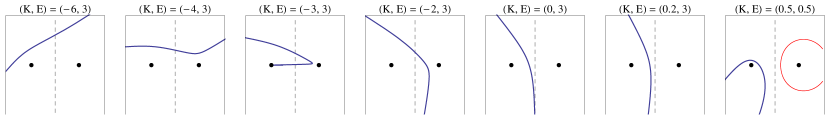
Figure 3.4: Example of possible motions in the case $Z_{+}=0$, $Z_{-}=2$ for values of $E$ and $K$ in different regions of the bifurcation diagram. The red line is the energy level of the trajectory in the plot.

3.4 Motion in the general case

We first describe the bifurcation set for the fully repelling (or attracting) configuration ${\rm sign}(Z_{1})={\rm sign}(Z_{2})$. The picture is similar to the one with $Z_{-}=0$ (see Section 3.2) with the only difference that some positive values of $K$ are allowed (see Figure 3.5).

Figure 3.5: Bifurcation diagrams for the fully attracting (left) and the fully repelling (right) case respectively. The shaded regions identify the complement of the Hill’s region.

Corollary 3.11.

Let $|Z_{+}|>Z_{-}$, $Z_{+}\in{\mathbb{R}}^{*}$, $Z_{-}\in{\mathbb{R}}^{0}_{+}$. With the notation of (3.5) we have

$${\mathcal{B}}({\mathcal{F}}){\mathbin{\upharpoonright}}\raise-2.15277pt\hbox{$\scriptstyle E\geq 0$}=\Big{\{}(E,K)\in{\mathcal{L}}_{0}\cup{\mathcal{L}}_{-}^{1}\cup{\mathcal{L}}_{-}^{2}\cup{\mathcal{L}}_{-}^{3}\cup{\mathcal{L}}_{+}^{2}\mid E\geq 0,K_{+}(E)\leq K\leq K_{-}(E)\Big{\}}.$$

Proof.

By Remark 3.6.2, ${\mathcal{L}}_{+}^{3}$ is not in the bifurcation set. The corollary follows immediately from Theorem 3.5. ∎

The structure of the trajectories and the qualitative behaviour of the motion in configuration space for this case is analogous to the one presented in Section 3.2, therefore we will not discuss it.

Figure 3.6: Bifurcation diagrams and labeled regions for $|Z_{+}|<Z_{-}$. The shaded regions identify the complement of the Hill’s region.

The case $|Z_{+}|<Z_{-}$ (that is, ${\rm sign}(Z_{1})\neq{\rm sign}(Z_{2})$) is particularly interesting, since for positive energies a set of bounded orbits of positive Liouville measure arises.

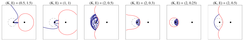
Figure 3.7: Bounded motions for $Z_{+}<0$, $|Z_{+}|<Z_{-}$ and $E\geq 0$. From left to right: trajectory for energy parameters on the boundary ${\mathcal{L}}^{2}_{+}$ of $I^{a}_{<}$, trajectory for energies on the tangency point between ${\mathcal{L}}^{2}_{+}$ and ${\mathcal{L}}_{+}^{3}$, trajectory for energies on the boundary ${\mathcal{L}}_{+}^{3}$ of $I^{a}_{<}$ Then follow two trajectories for energies inside $I_{<}^{a}$ and the trajectory on ${\mathcal{L}}^{3}_{+}$. The red line is the energy level of the trajectory in the plot, the dotted line is the $0$-energy level.

Corollary 3.12.

Let $|Z_{+}|<Z_{-}$, $Z_{+}\in{\mathbb{R}}^{*}$, $Z_{-}\in{\mathbb{R}}_{+}$. If $Z_{+}>0$ we have

$${\mathcal{B}}({\mathcal{F}}){\mathbin{\upharpoonright}}\raise-2.15277pt\hbox{$\scriptstyle E\geq 0$}=\Big{\{}(E,K)\in{\mathcal{L}}_{0}\cup{\mathcal{L}}_{-}^{1}\cup{\mathcal{L}}_{-}^{2}\cup{\mathcal{L}}_{-}^{3}\cup{\mathcal{L}}_{+}^{2}\mid E\geq 0\mbox{ and }K_{+}(E)\leq K\leq K_{-}(E)\Big{\}},$$

while if $Z_{+}<0$ we have

$${\mathcal{B}}({\mathcal{F}}){\mathbin{\upharpoonright}}\raise-2.15277pt\hbox{$\scriptstyle E\geq 0$}=\Big{\{}(E,K)\in{\mathcal{L}}_{0}\cup{\mathcal{L}}_{-}^{1}\cup{\mathcal{L}}_{-}^{2}\cup{\mathcal{L}}_{-}^{3}\cup{\mathcal{L}}_{+}^{2}\cup{\mathcal{L}}_{+}^{3}\mid E\geq 0\mbox{ and }K_{+}(E)\leq K\leq K_{-}(E)\Big{\}}.$$

Proof.

By Remark 3.6.2, ${\mathcal{L}}_{+}^{3}$ is in the bifurcation set for $Z_{+}<0$. The corollary follows immediately from Theorem 3.5. ∎

In this case the qualitative behaviour of the motion in configuration space is analogous to the one presented in Section 3.3, but for energy parameters in the region $I_{<}^{a}$. This region contains the set of energy parameters included in the region bounded above by ${\mathcal{L}}_{+}^{3-}:=\left\{(E,K)\in{\mathcal{L}}_{+}^{3}\;\middle|\;E<\frac{|Z_{+}|}{2}\right\}$, on the sides by ${\mathcal{L}}_{+}^{2}$ and ${\mathcal{L}}_{+}^{1}$ and below by $E\geq 0$ (see Fig. 3.6).

For $(E,V)$ on $I_{<}^{a}$ a new phenomenon appears: both the movable roots of $P_{+}(x)$ are bigger than one and the polynomial is non-negative in the union of the two disjoint intervals $[1,x_{3}]$ and $[x_{4},\infty)$. On the configuration space they give rise to an escaping trajectory similar to the previous ones and to a family of bounded trajectories near the attracting center (see Figure 3.7).

References

- [AM78] Ralph Abraham and Jerrold E. Marsden, Foundations of mechanics, Benjamin Cummings, 1978.
- [BCD87a] Ph. Briet, J.-M. Combes, and P. Duclos, On the location of resonances for Schrödinger operators in the semiclassical limit. I. Resonances free domains, J. Math. Anal. Appl. 126 (1987), no. 1, 90–99.
- [BCD87b] , On the location of resonances for Schrödinger operators in the semiclassical limit. II. Barrier top resonances, Communications in Partial Differential Equations 12 (1987), no. 2, 201–222.
- [BCD88] , Erratum for: on the location of resonance for Schrödinger operations in the semiclassical limit. II. Barrier top resonances, Communications in Partial Differential Equations 13 (1988), no. 3, 377–381.
- [CJK08] François Castella, Thierry Jecko, and Andreas Knauf, Semiclassical resolvent estimates for Schrödinger operators with Coulomb singularities, Ann. Henri Poincaré 9 (2008), no. 4, 775–815.
- [GS87] C. Gérard and J. Sjöstrand, Semiclassical resonances generated by a closed trajectory of hyperbolic type, Comm. Math. Phys. 108 (1987), no. 3, 391–421.
- [HM87] Bernard Helffer and André Martinez, Comparaison entre les diverses notions de résonances, Helv. Phys. Acta 60 (1987), no. 8, 992–1003.
- [HS96] P. D. Hislop and I. M. Sigal, Introduction to spectral theory, Applied Mathematical Sciences, vol. 113, Springer-Verlag, New York, 1996, With applications to Schrödinger operators.
- [Jac84] C. G. J. Jacobi, C.G.J. Jacobi’s Vorlesungen über Dynamik, G. Reimer, Berlin, 1884.
- [KK92] Marcus Klein and Andreas Knauf, Classical planar scattering by coulombic potentials, Lecture notes in physics: Monographs, no. v. 13, Springer, 1992.
- [Kna02] Andreas Knauf, The -centre problem of celestial mechanics for large energies, J. Eur. Math. Soc. (JEMS) 4 (2002), no. 1, 1–114.
- [Kna11] , Mathematische Physik: Klassische Mechanik, Springer-Lehrbuch Masterclass, Springer, 2011.
- [Mar02] A. Martinez, Resonance free domains for non globally analytic potentials, Ann. Henri Poincaré 3 (2002), no. 4, 739–756.
- [Mar07] , Erratum to: “Resonance free domains for non globally analytic potentials”, Ann. Henri Poincaré 8 (2007), no. 7, 1425–1431.
- [Pau22] Wolfgang Pauli, Über das Modell des Wasserstoffmolekülions, Annalen der Physik 373 (1922), no. 11, 177–240.
- [SAFG06] Tony C. Scott, Monique Aubert-Frécon, and Johannes Grotendorst, New approach for the electronic energies of the hydrogen molecular ion, Chemical Physics 324 (2006), no. 2–3, 323 – 338.
- [Ser12] M. Seri, Resonances in the two centers Coulomb system, www.opus.ub.uni-erlangen.de/opus/volltexte/2012/3546, Ph.D. thesis, Friedrich-Alexander-University Erlangen-Nuremberg, 09.2012.
- [Sjö87] Johannes Sjöstrand, Semiclassical resonances generated by nondegenerate critical points, Pseudodifferential operators (Oberwolfach, 1986), Lecture Notes in Math., vol. 1256, Springer, Berlin, 1987, pp. 402–429.
- [SKDEJ] M. Seri, A. Knauf, M. Degli Esposti, and T. Jecko, Resonances in the Two-Centers Coulomb System, preprint.
- [Thi88] W. Thirring, Lehrbuch der Mathematischen Physik 1, Springer, Wien, New York, 1988.
- [WDR04] Holger Waalkens, Holger R. Dullin, and Peter H. Richter, The problem of two fixed centers: bifurcations, actions, monodromy, Phys. D 196 (2004), no. 3-4, 265–310.
- [Zwo99] Maciej Zworski, Resonances in physics and geometry, Notices Amer. Math. Soc. 46 (1999), no. 3, 319–328.