Robust Clustering in Regression Analysis via the
Contaminated Gaussian Cluster-Weighted Model

Abstract

The Gaussian cluster-weighted model (CWM) is a mixture of regression models with random covariates that allows for flexible clustering of a random vector composed of response variables and covariates. In each mixture component, it adopts a Gaussian distribution for both the covariates and the responses given the covariates. To robustify the approach with respect to possible elliptical heavy tailed departures from normality, due to the presence of atypical observations, the contaminated Gaussian CWM is here introduced. In addition to the parameters of the Gaussian CWM, each mixture component of our contaminated CWM has a parameter controlling the proportion of outliers, one controlling the proportion of leverage points, one specifying the degree of contamination with respect to the response variables, and one specifying the degree of contamination with respect to the covariates. Crucially, these parameters do not have to be specified a priori, adding flexibility to our approach. Furthermore, once the model is estimated and the observations are assigned to the groups, a finer intra-group classification in typical points, outliers, good leverage points, and bad leverage points — concepts of primary importance in robust regression analysis — can be directly obtained. Relations with other mixture-based contaminated models are analyzed, identifiability conditions are provided, an expectation-conditional maximization algorithm is outlined for parameter estimation, and various implementation and operational issues are discussed. Properties of the estimators of the regression coefficients are evaluated through Monte Carlo experiments and compared to the estimators from the Gaussian CWM. A sensitivity study is also conducted based on a real data set.

capbtabboxtable[][]

1 Introduction

Given a continuous $d_{\boldsymbol{W}}$-variate random variable $\boldsymbol{W}$, with density $p\left(\boldsymbol{w}\right)$, finite mixtures of (continuous) distributions constitute both a flexible way for density estimation and a powerful device for clustering and classification by often assuming that each mixture component represents a group (or cluster or class) in the original data (see, e.g., Titterington et al., 1985, McLachlan and Basford, 1988, and McLachlan and Peel, 2000).

In many applied problems, the variable of interest $\boldsymbol{W}$ is composed by a $d_{\boldsymbol{Y}}$-variate response variable $\boldsymbol{Y}$ and by a random covariate $\boldsymbol{X}$ of dimension $d_{\boldsymbol{X}}$, with $d_{\boldsymbol{X}}+d_{\boldsymbol{Y}}=d_{\boldsymbol{W}}$; that is, $\boldsymbol{W}=\left(\boldsymbol{X},\boldsymbol{Y}\right)$. In such a case mixtures of distributions, that fail to incorporate a possible local (i.e., within-group) relation of $\boldsymbol{Y}$ on $\boldsymbol{X}=\boldsymbol{x}$, may perform inadequately. A valid alternative, in the mixture modeling framework, is represented by mixtures of regression models (see DeSarbo and Cron, 1988 and Frühwirth-Schnatter, 2006, Chapter 8 for details). In turn, this family of models can be split into two sub-families: mixtures of regression models with fixed covariates and mixtures of regression models with random covariates. However, as stated by Hennig (2000), the former subfamily is inadequate for most of the applications because it assumes “assignment independence”, i.e., that the probability for a point $\left(\boldsymbol{x},\boldsymbol{y}\right)$ to be generated by one of the groups distributions has to be the same for all covariate values $\boldsymbol{x}$. In other words, the assignment of the data points to the groups has to be independent of the covariates. On the contrary, mixtures of regression models with random covariates — which this paper focuses on — assume “assignment dependence” by allowing the assignment of the data points to the groups to depend on $\boldsymbol{X}$.

An eminent member in the class of mixtures of regression models with random covariates is represented by the cluster-weighted model (CWM; Gershenfeld, 1997), also called the saturated mixture regression model (Wedel, 2002). The CWM factorizes $p\left(\boldsymbol{x},\boldsymbol{y}\right)$, in each mixture component, into the product between the conditional density of $\boldsymbol{Y}|\boldsymbol{x}$ and the marginal density of $\boldsymbol{X}$ by assuming a local regression of $\boldsymbol{Y}$ on $\boldsymbol{x}$. The distribution of $\boldsymbol{X}$ can differ across groups and this allows for assignment dependence. Recent work on cluster-weighted modeling can be found in Ingrassia et al. (2012), Subedi et al. (2013), Ingrassia et al. (2014), and Punzo (2014). With respect to our framework, characterized by a possible multivariate response variable, Dang et al. (2014) propose the Gaussian CWM with density

$$p\left(\boldsymbol{x},\boldsymbol{y};\boldsymbol{\vartheta}\right)=\sum_{j=1}^{k}\pi_{j}\phi\left(\boldsymbol{y};\boldsymbol{\mu}_{\boldsymbol{Y}}\left(\boldsymbol{x};\boldsymbol{\beta}_{j}\right),\boldsymbol{\Sigma}_{\boldsymbol{Y}|j}\right)\phi\left(\boldsymbol{x};\boldsymbol{\mu}_{\boldsymbol{X}|j},\boldsymbol{\Sigma}_{\boldsymbol{X}|j}\right),$$ (1)

where $\pi_{j}$ are positive weights summing to one, $\phi\left(\cdot;\boldsymbol{\mu},\boldsymbol{\Sigma}\right)$ denotes the density of a Gaussian random vector with mean $\boldsymbol{\mu}$ and covariance matrix $\boldsymbol{\Sigma}$, and $\boldsymbol{\mu}_{\boldsymbol{Y}}\left(\boldsymbol{x};\boldsymbol{\beta}_{j}\right)=E\left(\boldsymbol{Y}|\boldsymbol{x},j\right)=\boldsymbol{\beta}_{j}^{\prime}\boldsymbol{x}^{*}$ denotes the local conditional mean of $\boldsymbol{Y}|\boldsymbol{x}$, with $\boldsymbol{\beta}_{j}$ being a vector of regression coefficients of dimension $\left[\left(1+d_{\boldsymbol{X}}\right)\times d_{\boldsymbol{Y}}\right]$ and $\boldsymbol{x}^{*}=\left(1,\boldsymbol{x}\right)$ to account for the intercept(s). In (1), $\boldsymbol{\vartheta}$ contains all of the parameters of the model.

Unfortunately, real data are often “contaminated” by atypical observations that affect the estimation of the model parameters with particular interest, in the regression context, to the regression coefficients. Accordingly, the detection of these atypical observations, and the development of robust methods of parameters estimation insensitive to their presence, is an important problem. However, as emphasized by Davies and Gather (1993) — see also Hennig, 2002 — atypical observations should be defined with respect to a reference distribution. That is, the shape (i.e., distribution) of the typical points has to be assumed in order to define what an atypical point is; in this way, the region of atypical points can be defined, e.g., as a region where the density of the reference distribution is low. If the reference distribution is chosen to be Gaussian, as for example in model (1), a common and simple elliptical generalization, having heavier tails for the occurrence of atypical points, is the contaminated Gaussian distribution; it is a two-component Gaussian mixture in which one of the components, with a large prior probability, represents the typical observations (reference distribution), and the other, with a small prior probability, the same mean, and an inflated covariance matrix, represents the atypical observations (Aitkin and Wilson, 1980).

Based on the above considerations, this paper introduces the contaminated Gaussian CWM, obtained from (1) by substituting the Gaussian distribution with the contaminated Gaussian distribution. Interestingly, each component joint density of the proposed model adheres to the taxonomy of atypical observations which is commonly considered in regression analysis; such a taxonomy will be recalled here (for further details see, e.g., Rousseeuw and Leroy, 2005, Chapter 1). In regression analysis, atypical observations can be distinguished between two types. Atypical observations in $\boldsymbol{Y}|\boldsymbol{x}$ represent model failure. Such observations are called (vertical) outliers. Atypical observations with respect to $\boldsymbol{X}$ are called leverage points. In regression it helps to make a distinction between two types of leverage points: good and bad. A bad leverage point is a regression outlier that has an $\boldsymbol{x}$ value that is atypical among the values of $\boldsymbol{X}$ as well. A good leverage point is a point that is unusually large or small among the $\boldsymbol{X}$ values but is not a regression outlier ($\boldsymbol{x}$ is atypical but the corresponding $\boldsymbol{y}$ fits the model quite well). A point like this is called “good” because it improves the precision of the regression coefficients (Rousseeuw and Van Zomeren, 1990, p. 635). Each point $\left(\boldsymbol{x},\boldsymbol{y}\right)$ can be so labeled in one of the four categories indicated in Table 1.

Table 1: Atypical observation labelling.

	Yes	No
Yes	bad leverage	outlier
No	good leverage	typical (bulk of the data)

As it will be better explained in Section 6.2, once the contaminated Gaussian CWM is fitted to the observed data, by means of maximum a posteriori probabilities, each observation can be first assigned to one of the $k$ groups and then classified into one of the four categories defined in Table 1; thus, we have a model for simultaneous clustering and detection of atypical observations in a regression context.

In the mixtures of regression models framework, other solutions for robust clustering exist. Some recent proposals are given in the following:

1. Galimberti and Soffritti (2014) propose a mixture of parallel regression models with $t$-distributed errors;

2. Yao et al. (2014) introduce mixtures of regression models with $t$-distributed errors;

3. Song et al. (2014) define mixtures of regression models with Laplace-distributed errors;

4. Ingrassia et al. (2012) propose the $t$ CWM, where the Gaussian distribution in (1) is replaced by a $t$ distribution (see also Ingrassia et al., 2014).

In general, with respect to our approach, these four models have some drawbacks. First, they do not allow for the direct detection of atypical observations. Actually, for the $t$-based models, a procedure described by McLachlan and Peel (2000, p. 232) could be eventually adopted to classify the observations as atypical. The procedure stems from a $\chi^{2}$-approximation of the squared Mahalanobis distance of each observation after its maximum a posteriori classification to one of the $k$ groups. However, the procedure is not direct and it is not corroborated by the theory. Second, the first three models do not consider the presence of possible leverage points in each group; moreover, they belong to the class of mixture of regression models with fixed covariates and, as such, assume assignment independence. The first model is also based on the assumption of parallel local regression models. It is also noteworthy that only the first model considers a possible multivariate response variable $\boldsymbol{Y}$. For further mixture-based approaches for robust clustering in regression analysis, see, e.g., Neykov et al. (2007) and Bai et al. (2012).

The paper is organized as follows. The contaminated Gaussian CWM is presented in Section 2 and compared to other mixture-based contaminated approaches in Section 3. Sufficient conditions for identifiability are given in Section 4, and an expectation-conditional maximization (ECM) algorithm for maximum likelihood parameter estimation is outlined in Section 5. Further operational aspects are discussed in Section 6. In Section 7.1, properties of the estimators of the regression coefficients $\boldsymbol{\beta}_{j}$ are evaluated through Monte Carlo experiments and compared to the estimators from the Gaussian CWM; a sensitivity study is also conducted in Section 7.2 based on a real data set. The paper concludes with some discussion in Section 8.

2 The model

A contaminated Gaussian distribution, for a real-valued random vector $\boldsymbol{W}$, is given by

$$f\left(\boldsymbol{w};\boldsymbol{\mu}_{\boldsymbol{W}},\boldsymbol{\Sigma}_{\boldsymbol{W}},\alpha_{\boldsymbol{W}},\eta_{\boldsymbol{W}}\right)=\alpha_{\boldsymbol{W}}\phi\left(\boldsymbol{w};\boldsymbol{\mu}_{\boldsymbol{W}},\boldsymbol{\Sigma}_{\boldsymbol{W}}\right)+\left(1-\alpha_{\boldsymbol{W}}\right)\phi\left(\boldsymbol{w};\boldsymbol{\mu}_{\boldsymbol{W}},\eta_{\boldsymbol{W}}\boldsymbol{\Sigma}_{\boldsymbol{W}}\right),$$ (2)

where $\alpha_{\boldsymbol{W}}\in\left(0,1\right)$ and $\eta_{\boldsymbol{W}}>1$. In (2), $\eta_{\boldsymbol{W}}$ denotes the degree of contamination, and because of the assumption $\eta_{\boldsymbol{W}}>1$, it can be interpreted as the increase in variability due to the bad observations (i.e., it is an inflation parameter). As a limiting case, when $\alpha_{\boldsymbol{W}}\rightarrow 1^{-}$ and $\eta_{\boldsymbol{W}}\rightarrow 1^{+}$, the Gaussian distribution is obtained.

A common and different way to burden the Gaussian tails (reference distribution), still maintaining ellipticity, is represented by the $t$ distribution (see Kotz and Nadarajah, 2004 and Lange et al., 1989 for details). An advantage of model (2) with respect to the $t$ model is that, once the parameters are estimated, say $\hat{\boldsymbol{\mu}}_{\boldsymbol{W}}$, $\hat{\boldsymbol{\Sigma}}_{\boldsymbol{W}}$, $\hat{\alpha}_{\boldsymbol{W}}$, and $\hat{\eta}_{\boldsymbol{W}}$, we can establish if a generic observation $\boldsymbol{w}$ is either good or bad, with respect to the reference distribution, by means of the a posteriori probability

$$P\left(\text{$\boldsymbol{w}$ is good}\left|\hat{\boldsymbol{\mu}}_{\boldsymbol{W}},\hat{\boldsymbol{\Sigma}}_{\boldsymbol{W}},\hat{\alpha}_{\boldsymbol{W}},\hat{\eta}_{\boldsymbol{W}}\right.\right)=\hat{\alpha}\phi\left(\boldsymbol{w};\hat{\boldsymbol{\mu}},\hat{\boldsymbol{\Sigma}}\right)\Big{/}f\left(\boldsymbol{w};\hat{\boldsymbol{\mu}}_{\boldsymbol{W}},\hat{\boldsymbol{\Sigma}}_{\boldsymbol{W}},\hat{\alpha}_{\boldsymbol{W}},\hat{\eta}_{\boldsymbol{W}}\right),$$

and $\boldsymbol{w}$ will be considered good if $P\left(\text{$\boldsymbol{w}$ is good}\left|\hat{\boldsymbol{\mu}}_{\boldsymbol{W}},\hat{\boldsymbol{\Sigma}}_{\boldsymbol{W}},\hat{\alpha}_{\boldsymbol{W}},\hat{\eta}_{\boldsymbol{W}}\right.\right)\geq 1/2$, while it will be considered bad otherwise.

Based on model (2), Punzo and McNicholas (2014a) introduce, for robust model-based clustering, finite mixtures of contaminated Gaussian distributions with density

$$p\left(\boldsymbol{w};\boldsymbol{\vartheta}\right)=\sum_{j=1}^{k}\pi_{j}f\left(\boldsymbol{w};\boldsymbol{\mu}_{\boldsymbol{W}|j},\boldsymbol{\Sigma}_{\boldsymbol{W}|j},\alpha_{\boldsymbol{W}|j},\eta_{\boldsymbol{W}|j}\right).$$ (3)

Unfortunately, with respect to the framework of this paper, model (3) does not account for local relations of the response $\boldsymbol{Y}$ on the covariate $\boldsymbol{X}=\boldsymbol{x}$ when $\boldsymbol{W}=\left(\boldsymbol{X},\boldsymbol{Y}\right)$. However, in a context of mixtures of regression models with fixed covariates, the contaminated Gaussian distribution can be also considered to model $\boldsymbol{Y}|\boldsymbol{x}$ in each mixture component; this leads to the mixture of contaminated Gaussian regression models

$$p\left(\boldsymbol{y}|\boldsymbol{x};\boldsymbol{\vartheta}\right)=\sum_{j=1}^{k}\pi_{j}f\left(\boldsymbol{y};\boldsymbol{\mu}_{\boldsymbol{Y}}\left(\boldsymbol{x};\boldsymbol{\beta}_{j}\right),\boldsymbol{\Sigma}_{\boldsymbol{Y}|j},\alpha_{\boldsymbol{Y}|j},\eta_{\boldsymbol{Y}|j}\right).$$ (4)

However, because model (4) belongs to the class of mixtures of regression models with fixed covariates, it suffers from the assignment independence property. Moreover, it can not be used to detect local leverage points (cf. Section 1).

To improve model (4), we propose the contaminated Gaussian CWM; it is obtained by replacing the Gaussian distribution in model (1) with the contaminated Gaussian distribution. This yields

$$p\left(\boldsymbol{x},\boldsymbol{y};\boldsymbol{\vartheta}\right)=\sum_{j=1}^{k}\pi_{j}f\left(\boldsymbol{y};\boldsymbol{\mu}_{\boldsymbol{Y}}\left(\boldsymbol{x};\boldsymbol{\beta}_{j}\right),\boldsymbol{\Sigma}_{\boldsymbol{Y}|j},\alpha_{\boldsymbol{Y}|j},\eta_{\boldsymbol{Y}|j}\right)f\left(\boldsymbol{x};\boldsymbol{\mu}_{\boldsymbol{X}|j},\boldsymbol{\Sigma}_{\boldsymbol{X}|j},\alpha_{\boldsymbol{X}|j},\eta_{\boldsymbol{X}|j}\right).$$ (5)

3 Relation with other contaminated models

The contaminated Gaussian CWM defined in (5) can be related to the mixture-based contaminated models defined in Section 2.

3.1 Comparison with the mixture of contaminated Gaussian distributions

To begin, we consider the comparison with mixtures of contaminated Gaussian distributions. With this aim, it is convenient to write the parameters $\boldsymbol{\mu}_{\boldsymbol{W}|j}$ and $\boldsymbol{\Sigma}_{\boldsymbol{W}|j}$, $j=1,\ldots,k$, of the mixture of contaminated Gaussian distributions defined in (3) as

$$\boldsymbol{\mu}_{\boldsymbol{W}|j}=\begin{pmatrix}\boldsymbol{\mu}_{\boldsymbol{X}|j}\\ \boldsymbol{\mu}_{\boldsymbol{Y}|j}\end{pmatrix}\quad\text{and}\quad\boldsymbol{\Sigma}_{\boldsymbol{W}|j}=\begin{pmatrix}\boldsymbol{\Sigma}_{\boldsymbol{X}\boldsymbol{X}|j}&\boldsymbol{\Sigma}_{\boldsymbol{X}\boldsymbol{Y}|j}\\ \boldsymbol{\Sigma}_{\boldsymbol{Y}\boldsymbol{X}|j}&\boldsymbol{\Sigma}_{\boldsymbol{Y}\boldsymbol{Y}|j}\end{pmatrix}.$$

Based on well-known results about marginal and conditional distributions from a multivariate Gaussian random vector (see, e.g., Mardia et al., 1997), model (3) can be rewritten as

$$p\left(\boldsymbol{w};\boldsymbol{\vartheta}\right)=\sum_{j=1}^{k}\pi_{j} f\left(\boldsymbol{w};\boldsymbol{\mu}_{\boldsymbol{W}|j},\boldsymbol{\Sigma}_{\boldsymbol{W}|j},\alpha_{\boldsymbol{W}|j},\eta_{\boldsymbol{W}|j}\right)=\sum_{j=1}^{k}\pi_{j}\left[\alpha_{\boldsymbol{W}|j}\phi\left(\boldsymbol{w};\boldsymbol{\mu}_{\boldsymbol{W}|j},\boldsymbol{\Sigma}_{\boldsymbol{W}|j}\right)+\left(1-\alpha_{\boldsymbol{W}|j}\right)\phi\left(\boldsymbol{w};\boldsymbol{\mu}_{\boldsymbol{W}|j},\eta_{\boldsymbol{W}|j}\boldsymbol{\Sigma}_{\boldsymbol{W}|j}\right)\right]$$

$$=\sum_{j=1}^{k}\pi_{j} \Bigg{[}\frac{\alpha_{\boldsymbol{W}|j}\phi\left(\boldsymbol{x};\boldsymbol{\mu}_{\boldsymbol{X}|j},\boldsymbol{\Sigma}_{\boldsymbol{X}\boldsymbol{X}|j}\right)}{\alpha_{\boldsymbol{W}|j}\phi\left(\boldsymbol{x};\boldsymbol{\mu}_{\boldsymbol{X}|j},\boldsymbol{\Sigma}_{\boldsymbol{X}\boldsymbol{X}|j}\right)+\left(1-\alpha_{\boldsymbol{W}|j}\right)\phi\left(\boldsymbol{x};\boldsymbol{\mu}_{\boldsymbol{X}|j},\eta_{\boldsymbol{W}|j}\boldsymbol{\Sigma}_{\boldsymbol{X}\boldsymbol{X}|j}\right)}\phi\left(\boldsymbol{y};\boldsymbol{\mu}_{\boldsymbol{Y}|\boldsymbol{X},j},\boldsymbol{\Sigma}_{\boldsymbol{Y}\boldsymbol{Y}|j}\right)$$

$$+\frac{\left(1-\alpha_{\boldsymbol{W}|j}\right)\phi\left(\boldsymbol{x};\boldsymbol{\mu}_{\boldsymbol{X}|j},\eta_{\boldsymbol{W}|j}\boldsymbol{\Sigma}_{\boldsymbol{X}\boldsymbol{X}|j}\right)}{\alpha_{\boldsymbol{W}|j}\phi\left(\boldsymbol{x};\boldsymbol{\mu}_{\boldsymbol{X}|j},\boldsymbol{\Sigma}_{\boldsymbol{X}\boldsymbol{X}|j}\right)+\left(1-\alpha_{\boldsymbol{W}|j}\right)\phi\left(\boldsymbol{x};\boldsymbol{\mu}_{\boldsymbol{X}|j},\eta_{\boldsymbol{W}|j}\boldsymbol{\Sigma}_{\boldsymbol{X}\boldsymbol{X}|j}\right)}\phi\left(\boldsymbol{y};\boldsymbol{\mu}_{\boldsymbol{Y}|\boldsymbol{X},j},\eta_{\boldsymbol{W}|j}\boldsymbol{\Sigma}_{\boldsymbol{Y}\boldsymbol{Y}|j}\right)\Bigg{]}$$

$$\times\left[\alpha_{\boldsymbol{W}|j}\phi\left(\boldsymbol{x};\boldsymbol{\mu}_{\boldsymbol{X}|j},\boldsymbol{\Sigma}_{\boldsymbol{X}\boldsymbol{X}|j}\right)+\left(1-\alpha_{\boldsymbol{W}|j}\right)\phi\left(\boldsymbol{x};\boldsymbol{\mu}_{\boldsymbol{X}|j},\eta_{\boldsymbol{W}|j}\boldsymbol{\Sigma}_{\boldsymbol{X}\boldsymbol{X}|j}\right)\right]$$

$$=\sum_{j=1}^{k}\pi_{j} \Big{[}\alpha_{\boldsymbol{W}|j}\phi\left(\boldsymbol{x};\boldsymbol{\mu}_{\boldsymbol{X}|j},\boldsymbol{\Sigma}_{\boldsymbol{X}\boldsymbol{X}|j}\right)\phi\left(\boldsymbol{y};\boldsymbol{\mu}_{\boldsymbol{Y}|\boldsymbol{X},j},\boldsymbol{\Sigma}_{\boldsymbol{Y}\boldsymbol{Y}|j}\right)$$

$$+\left(1-\alpha_{\boldsymbol{W}|j}\right)\phi\left(\boldsymbol{x};\boldsymbol{\mu}_{\boldsymbol{X}|j},\eta_{\boldsymbol{W}|j}\boldsymbol{\Sigma}_{\boldsymbol{X}\boldsymbol{X}|j}\right)\phi\left(\boldsymbol{y};\boldsymbol{\mu}_{\boldsymbol{Y}|\boldsymbol{X},j},\eta_{\boldsymbol{W}|j}\boldsymbol{\Sigma}_{\boldsymbol{Y}\boldsymbol{Y}|j}\right)\Big{]},$$ (6)

where

$$\boldsymbol{\mu}_{\boldsymbol{Y}|\boldsymbol{X},j}=\boldsymbol{\mu}_{\boldsymbol{Y}|j}+\boldsymbol{\Sigma}_{\boldsymbol{Y}\boldsymbol{X}|j}\boldsymbol{\Sigma}_{\boldsymbol{X}\boldsymbol{X}|j}^{-1}\left(\boldsymbol{x}-\boldsymbol{\mu}_{\boldsymbol{X}|j}\right)$$

is a linear function of $\boldsymbol{x}$. For comparison’s sake, it is also convenient to write model (5) as

$$p\left(\boldsymbol{x},\boldsymbol{y};\boldsymbol{\vartheta}\right)=\sum_{j=1}^{k}\pi_{j} f\left(\boldsymbol{y};\boldsymbol{\mu}_{\boldsymbol{Y}}\left(\boldsymbol{x};\boldsymbol{\beta}_{j}\right),\boldsymbol{\Sigma}_{\boldsymbol{Y}|j},\alpha_{\boldsymbol{Y}|j},\eta_{\boldsymbol{Y}|j}\right)f\left(\boldsymbol{x};\boldsymbol{\mu}_{\boldsymbol{X}|j},\boldsymbol{\Sigma}_{\boldsymbol{X}|j},\alpha_{\boldsymbol{X}|j},\eta_{\boldsymbol{X}|j}\right)$$

$$=\sum_{j=1}^{k}\pi_{j} \left[\alpha_{\boldsymbol{Y}|j}\phi\left(\boldsymbol{y};\boldsymbol{\mu}_{\boldsymbol{Y}}\left(\boldsymbol{x};\boldsymbol{\beta}_{j}\right),\boldsymbol{\Sigma}_{\boldsymbol{Y}|j}\right)+\left(1-\alpha_{\boldsymbol{Y}|j}\right)\phi\left(\boldsymbol{y};\boldsymbol{\mu}_{\boldsymbol{Y}}\left(\boldsymbol{x};\boldsymbol{\beta}_{j}\right),\eta_{\boldsymbol{Y}|j}\boldsymbol{\Sigma}_{\boldsymbol{Y}|j}\right)\right]$$

$$\times\left[\alpha_{\boldsymbol{X}|j}\phi\left(\boldsymbol{x};\boldsymbol{\mu}_{\boldsymbol{X}|j},\boldsymbol{\Sigma}_{\boldsymbol{X}|j}\right)+\left(1-\alpha_{\boldsymbol{X}|j}\right)\phi\left(\boldsymbol{x};\boldsymbol{\mu}_{\boldsymbol{X}|j},\eta_{\boldsymbol{X}|j}\boldsymbol{\Sigma}_{\boldsymbol{X}|j}\right)\right]$$

$$=\sum_{j=1}^{k}\pi_{j} \Big{[}\alpha_{\boldsymbol{X}|j}\alpha_{\boldsymbol{Y}|j}\phi\left(\boldsymbol{x};\boldsymbol{\mu}_{\boldsymbol{X}|j},\boldsymbol{\Sigma}_{\boldsymbol{X}|j}\right)\phi\left(\boldsymbol{y};\boldsymbol{\mu}_{\boldsymbol{Y}}\left(\boldsymbol{x};\boldsymbol{\beta}_{j}\right),\boldsymbol{\Sigma}_{\boldsymbol{Y}|j}\right)$$

$$+\alpha_{\boldsymbol{X}|j}\left(1-\alpha_{\boldsymbol{Y}|j}\right)\phi\left(\boldsymbol{x};\boldsymbol{\mu}_{\boldsymbol{X}|j},\boldsymbol{\Sigma}_{\boldsymbol{X}|j}\right)\phi\left(\boldsymbol{y};\boldsymbol{\mu}_{\boldsymbol{Y}}\left(\boldsymbol{x};\boldsymbol{\beta}_{j}\right),\eta_{\boldsymbol{Y}|j}\boldsymbol{\Sigma}_{\boldsymbol{Y}|j}\right)$$

$$+\left(1-\alpha_{\boldsymbol{X}|j}\right)\alpha_{\boldsymbol{Y}|j}\phi\left(\boldsymbol{x};\boldsymbol{\mu}_{\boldsymbol{X}|j},\eta_{\boldsymbol{X}|j}\boldsymbol{\Sigma}_{\boldsymbol{X}|j}\right)\phi\left(\boldsymbol{y};\boldsymbol{\mu}_{\boldsymbol{Y}}\left(\boldsymbol{x};\boldsymbol{\beta}_{j}\right),\boldsymbol{\Sigma}_{\boldsymbol{Y}|j}\right)$$

$$+\left(1-\alpha_{\boldsymbol{X}|j}\right)\left(1-\alpha_{\boldsymbol{Y}|j}\right)\phi\left(\boldsymbol{x};\boldsymbol{\mu}_{\boldsymbol{X}|j},\eta_{\boldsymbol{X}|j}\boldsymbol{\Sigma}_{\boldsymbol{X}|j}\right)\phi\left(\boldsymbol{y};\boldsymbol{\mu}_{\boldsymbol{Y}}\left(\boldsymbol{x};\boldsymbol{\beta}_{j}\right),\eta_{\boldsymbol{Y}|j}\boldsymbol{\Sigma}_{\boldsymbol{Y}|j}\right)\Big{]}.$$ (7)

Comparing the expressions enclosed within square brackets at the end of (6) with the equivalent term in (7), it is straightforward to realize the difference between the models.

3.2 Comparison with the mixture of contaminated Gaussian regressions

The second comparison concerns mixtures of contaminated Gaussian regression models as defined in (4). The comparison is not direct because, while model (4) is defined on the conditional distribution $p\left(\boldsymbol{y}|\boldsymbol{x}\right)$, model (5) is defined on the joint distribution $p\left(\boldsymbol{x},\boldsymbol{y}\right)$. Although we can not compute $p\left(\boldsymbol{x},\boldsymbol{y}\right)$ from a mixture of regression models with fixed covariates because this class of models does not consider modeling for the marginal distribution $p\left(\boldsymbol{x}\right)$, we can still compute the conditional distribution $p\left(\boldsymbol{y}|\boldsymbol{x}\right)$ from the contaminated Gaussian CWM. In particular, by integrating out $\boldsymbol{y}$ from model (5) we obtain

$$p\left(\boldsymbol{x};\boldsymbol{\vartheta}\right)=\sum_{j=1}^{k}\pi_{j}f\left(\boldsymbol{x};\boldsymbol{\mu}_{\boldsymbol{X}|j},\boldsymbol{\Sigma}_{\boldsymbol{X}|j},\alpha_{\boldsymbol{X}|j},\eta_{\boldsymbol{X}|j}\right);$$ (8)

this is a mixture of contaminated Gaussian distributions for the $\boldsymbol{X}$ only. The ratio of (5) over (8) yields

$$p\left(\boldsymbol{y}|\boldsymbol{x};\boldsymbol{\vartheta}\right)=\sum_{j=1}^{k}\frac{\pi_{j}f\left(\boldsymbol{x};\boldsymbol{\mu}_{\boldsymbol{X}|j},\boldsymbol{\Sigma}_{\boldsymbol{X}|j},\alpha_{\boldsymbol{X}|j},\eta_{\boldsymbol{X}|j}\right)}{\displaystyle\sum_{h=1}^{k}\pi_{h}f\left(\boldsymbol{x};\boldsymbol{\mu}_{\boldsymbol{X}|h},\boldsymbol{\Sigma}_{\boldsymbol{X}|h},\alpha_{\boldsymbol{X}|h},\eta_{\boldsymbol{X}|h}\right)}f\left(\boldsymbol{y};\boldsymbol{\mu}_{\boldsymbol{Y}}\left(\boldsymbol{x};\boldsymbol{\beta}_{j}\right),\boldsymbol{\Sigma}_{\boldsymbol{Y}|j},\alpha_{\boldsymbol{Y}|j},\eta_{\boldsymbol{Y}|j}\right).$$ (9)

Model (9) is the conditional distribution of $\boldsymbol{Y}|\boldsymbol{x}$ from a contaminated Gaussian CWM; it can be seen as a mixture of regression models with (dynamic) weights depending on $\boldsymbol{x}$.

The following proposition shows as the family of mixtures of contaminated Gaussian regression models can be seen as nested in the family of contaminated Gaussian CWMs, as defined by (9).

Proposition 1.

If, in (9), $\boldsymbol{\mu}_{\boldsymbol{X}|1}=\cdots=\boldsymbol{\mu}_{\boldsymbol{X}|k}=\boldsymbol{\mu}_{\boldsymbol{X}}$, $\boldsymbol{\Sigma}_{\boldsymbol{X}|1}=\cdots=\boldsymbol{\Sigma}_{\boldsymbol{X}|k}=\boldsymbol{\Sigma}_{\boldsymbol{X}}$, $\alpha_{\boldsymbol{X}|1}=\cdots=\alpha_{\boldsymbol{X}|k}=\alpha_{\boldsymbol{X}}$, and $\eta_{\boldsymbol{X}|1}=\cdots=\eta_{\boldsymbol{X}|k}=\eta_{\boldsymbol{X}}$, then mixtures of contaminated Gaussian regression models, as defined by (4), can be seen as a particular case of the contaminated Gaussian CWM, as defined by (9).

Proof. A proof of this proposition is provided in A. ∎

4 Identifiability

Before outlining maximum likelihood (ML) parameter estimation for model (5), it is important to establish its identifiability, that is, two sets of parameters in the model, say $\boldsymbol{\vartheta}$ and $\widetilde{\boldsymbol{\vartheta}}$, which do not agree after permutation cannot yield the same mixture distribution. Identifiability is a necessary requirement, inter alia, for the usual asymptotic theory to hold for ML estimation of the model parameters (cf. Section 5).

General conditions for the identifiability of mixtures of (linear Gaussian) regression models with fixed and random covariates are provided in Hennig (2000). A sufficient condition for the identifiability of the mixture of contaminated Gaussian distributions is given in Punzo and McNicholas (2014a). These results will be used in Proposition 2 to show that model (5) is identifiable provided that all pairs $\left(\boldsymbol{\beta}_{j},\boldsymbol{\Sigma}_{\boldsymbol{Y}|j}\right)$, $j=1,\ldots,k$, are pairwise distinct. Note that, the positivity of all the weights $\pi_{j}$ avoids nonidentifiability due to empty components (see Frühwirth-Schnatter, 2006, Section 1.3.3 for details).

Proposition 2.

Let

$$p\left(\boldsymbol{x},\boldsymbol{y};\boldsymbol{\vartheta}\right)=\sum_{j=1}^{k}\pi_{j}f\left(\boldsymbol{y};\boldsymbol{\mu}_{\boldsymbol{Y}}\left(\boldsymbol{x};\boldsymbol{\beta}_{j}\right),\boldsymbol{\Sigma}_{\boldsymbol{Y}|j},\alpha_{\boldsymbol{Y}|j},\eta_{\boldsymbol{Y}|j}\right)f\left(\boldsymbol{x};\boldsymbol{\mu}_{\boldsymbol{X}|j},\boldsymbol{\Sigma}_{\boldsymbol{X}|j},\alpha_{\boldsymbol{X}|j},\eta_{\boldsymbol{X}|j}\right).$$

and

$$p\left(\boldsymbol{x},\boldsymbol{y};\widetilde{\boldsymbol{\vartheta}}\right)=\sum_{s=1}^{\widetilde{k}}\widetilde{\pi}_{s}f\left(\boldsymbol{y};\boldsymbol{\mu}_{\boldsymbol{Y}}\left(\boldsymbol{x};\widetilde{\boldsymbol{\beta}}_{s}\right),\widetilde{\boldsymbol{\Sigma}}_{\boldsymbol{Y}|s},\widetilde{\alpha}_{\boldsymbol{Y}|s},\widetilde{\eta}_{\boldsymbol{Y}|s}\right)f\left(\boldsymbol{x};\widetilde{\boldsymbol{\mu}}_{\boldsymbol{X}|s},\widetilde{\boldsymbol{\Sigma}}_{\boldsymbol{X}|s},\widetilde{\alpha}_{\boldsymbol{X}|s},\widetilde{\eta}_{\boldsymbol{X}|s}\right).$$

be two different parameterizations of the contaminated Gaussian CWM given in (5). If $j\neq l$, with $j,l\in\left\{1,\ldots,k\right\}$, implies

$$\left\|\boldsymbol{\beta}_{j}-\boldsymbol{\beta}_{l}\right\|_{2}^{2}+\left\|\boldsymbol{\Sigma}_{\boldsymbol{Y}|j}-a\boldsymbol{\Sigma}_{\boldsymbol{Y}|l}\right\|_{2}^{2}\neq 0$$ (10)

for all $a>0$, where $\left\|\cdot\right\|_{2}$ is the Froebenius norm, then the equality $p\left(\boldsymbol{x},\boldsymbol{y};\boldsymbol{\vartheta}\right)=p\left(\boldsymbol{x},\boldsymbol{y};\widetilde{\boldsymbol{\vartheta}}\right)$, for almost all $\boldsymbol{x}\in^{d_{\boldsymbol{X}}}$, implies that $k=\widetilde{k}$ and also implies that for each $j\in\left\{1,\ldots,k\right\}$ there exists an $s\in\left\{1,\ldots,k\right\}$ such that $\pi_{j}=\widetilde{\pi}_{s}$, $\alpha_{\boldsymbol{X}|j}=\widetilde{\alpha}_{\boldsymbol{X}|s}$, $\boldsymbol{\mu}_{\boldsymbol{X}|j}=\widetilde{\boldsymbol{\mu}}_{\boldsymbol{X}|s}$, $\boldsymbol{\Sigma}_{\boldsymbol{X}|j}=\widetilde{\boldsymbol{\Sigma}}_{\boldsymbol{X}|s}$, $\eta_{\boldsymbol{X}|j}=\widetilde{\eta}_{\boldsymbol{X}|s}$, $\alpha_{\boldsymbol{Y}|j}=\widetilde{\alpha}_{\boldsymbol{Y}|s}$, $\boldsymbol{\beta}_{j}=\widetilde{\boldsymbol{\beta}}_{s}$, $\boldsymbol{\Sigma}_{\boldsymbol{Y}|j}=\widetilde{\boldsymbol{\Sigma}}_{\boldsymbol{Y}|s}$, and $\eta_{\boldsymbol{Y}|j}=\widetilde{\eta}_{\boldsymbol{Y}|s}$.

Proof. A proof of this proposition is provided in B. ∎

5 Maximum likelihood estimation

5.1 An ECM algorithm

Let $\left(\boldsymbol{x}_{1},\boldsymbol{y}_{1}\right),\ldots,\left(\boldsymbol{x}_{n},\boldsymbol{y}_{n}\right)$ be a sample from model (5). To find ML estimates for the parameters of this model, we adopt the expectation-conditional maximization (ECM) algorithm of Meng and Rubin (1993). The ECM algorithm is a variant of the classical expectation-maximization (EM) algorithm (Dempster et al., 1977), which is a natural approach for ML estimation when data are incomplete. In our case, there are three sources of incompleteness. The first source, the classical one in the use of mixture models, arise from the fact that for each observation we do not know its component membership; this source is governed by an indicator vector $\boldsymbol{z}_{i}=\left(z_{i1},\ldots,z_{ik}\right)$, where $z_{i1}=1$ if $\left(\boldsymbol{x}_{i},\boldsymbol{y}_{i}\right)$ comes from component $j$ and $z_{ij}=0$ otherwise. The other two sources, which are specific for this model, arise from the fact that for each observation we do not know if it is an outlier and/or a leverage point with reference to component $j$ (cf. Table 1). To denote these sources of incompleteness, we use $\boldsymbol{u}_{i}=\left(u_{i1},\ldots,u_{ik}\right)$, where $u_{ij}=1$ if $\left(\boldsymbol{x}_{i},\boldsymbol{y}_{i}\right)$ is not an outlier in component $j$ and $u_{ij}=0$ otherwise, and $\boldsymbol{v}_{i}=\left(v_{i1},\ldots,v_{ik}\right)$, where $v_{ij}=1$ if $\left(\boldsymbol{x}_{i},\boldsymbol{y}_{i}\right)$ is not a leverage point in component $j$ and $v_{ij}=0$ otherwise. Therefore, complete-data likelihood can be written

$$L_{c}\left(\boldsymbol{\vartheta}\right)=\prod_{i=1}^{n}\prod_{j=1}^{k}\Bigg{\{} \pi_{j}\left[\alpha_{\boldsymbol{X}|j}\phi\left(\boldsymbol{x};\boldsymbol{\mu}_{\boldsymbol{X}|j},\boldsymbol{\Sigma}_{\boldsymbol{X}|j}\right)\right]^{v_{ij}}\left[\left(1-\alpha_{\boldsymbol{X}|j}\right)\phi\left(\boldsymbol{y};\boldsymbol{\mu}_{\boldsymbol{X}|j},\eta_{\boldsymbol{X}|j}\boldsymbol{\Sigma}_{\boldsymbol{X}|j}\right)\right]^{1-v_{ij}}$$

$$\times\left[\alpha_{\boldsymbol{Y}|j}\phi\left(\boldsymbol{y};\boldsymbol{\mu}_{\boldsymbol{Y}}\left(\boldsymbol{x}_{i};\boldsymbol{\beta}_{j}\right),\boldsymbol{\Sigma}_{\boldsymbol{Y}|j}\right)\right]^{u_{ij}}\left[\left(1-\alpha_{\boldsymbol{Y}|j}\right)\phi\left(\boldsymbol{y};\boldsymbol{\mu}_{\boldsymbol{Y}}\left(\boldsymbol{x}_{i};\boldsymbol{\beta}_{j}\right),\eta_{\boldsymbol{Y}|j}\boldsymbol{\Sigma}_{\boldsymbol{Y}|j}\right)\right]^{1-u_{ij}}\Bigg{\}}^{z_{ij}}.$$

Therefore, the complete-data log-likelihood, which is the core of the algorithm, becomes

$$l_{c}\left(\boldsymbol{\vartheta}\right)=l_{1c}\left(\boldsymbol{\pi}\right)+l_{2c}\left(\boldsymbol{\alpha}_{\boldsymbol{X}}\right)+l_{3c}\left(\boldsymbol{\mu}_{\boldsymbol{X}},\boldsymbol{\Sigma}_{\boldsymbol{X}},\boldsymbol{\eta}_{\boldsymbol{X}}\right)+l_{4c}\left(\boldsymbol{\alpha}_{\boldsymbol{Y}}\right)+l_{5c}\left(\boldsymbol{\beta},\boldsymbol{\Sigma}_{\boldsymbol{Y}},\boldsymbol{\eta}_{\boldsymbol{Y}}\right),$$ (11)

where $\boldsymbol{\pi}=\left(\pi_{1},\ldots,\pi_{k}\right)$, $\boldsymbol{\mu}_{\boldsymbol{X}}=\left(\boldsymbol{\mu}_{\boldsymbol{X}|1},\ldots,\boldsymbol{\mu}_{\boldsymbol{X}|k}\right)$, $\boldsymbol{\Sigma}_{\boldsymbol{X}}=\left(\boldsymbol{\Sigma}_{\boldsymbol{X}|1},\ldots,\boldsymbol{\Sigma}_{\boldsymbol{X}|k}\right)$, $\boldsymbol{\alpha}_{\boldsymbol{X}}=\left(\alpha_{\boldsymbol{X}|1},\ldots,\alpha_{\boldsymbol{X}|k}\right)$, $\boldsymbol{\eta}_{\boldsymbol{X}}=\left(\eta_{\boldsymbol{X}|1},\ldots,\eta_{\boldsymbol{X}|k}\right)$, $\boldsymbol{\beta}=\left(\boldsymbol{\beta}_{1},\ldots,\boldsymbol{\beta}_{k}\right)$, $\boldsymbol{\Sigma}_{\boldsymbol{Y}}=\left(\boldsymbol{\Sigma}_{\boldsymbol{Y}|1},\ldots,\boldsymbol{\Sigma}_{\boldsymbol{Y}|k}\right)$, $\boldsymbol{\alpha}_{\boldsymbol{Y}}=\left(\alpha_{\boldsymbol{Y}|1},\ldots,\alpha_{\boldsymbol{Y}|k}\right)$, $\boldsymbol{\eta}_{\boldsymbol{Y}}=\left(\eta_{\boldsymbol{Y}|1},\ldots,\eta_{\boldsymbol{Y}|k}\right)$,

$$l_{1c}\left(\boldsymbol{\pi}\right)=\sum_{i=1}^{n}\sum_{j=1}^{k}{z}_{ij}\ln\pi_{j},\qquad\qquad l_{2c}\left(\boldsymbol{\alpha}_{\boldsymbol{Y}}\right)=\sum_{i=1}^{n}\sum_{j=1}^{k}z_{ij}\left[v_{ij}\ln\alpha_{\boldsymbol{X}|j}+\left(1-v_{ij}\right)\ln\left(1-\alpha_{\boldsymbol{X}|j}\right)\right],$$

$$l_{3c}\left(\boldsymbol{\mu}_{\boldsymbol{X}},\boldsymbol{\Sigma}_{\boldsymbol{X}},\boldsymbol{\eta}_{\boldsymbol{X}}\right)=-\frac{1}{2}\sum_{i=1}^{n}\sum_{j=1}^{k}\Biggl{\{}z_{ij}\ln\left|\boldsymbol{\Sigma}_{\boldsymbol{X}|j}\right|+d_{\boldsymbol{X}}z_{ij}\left(1-v_{ij}\right)\ln\eta_{\boldsymbol{X}|j}+z_{ij}\left(v_{ij}+\frac{1-v_{ij}}{\eta_{\boldsymbol{X}|j}}\right)\delta\left(\boldsymbol{x}_{i},\boldsymbol{\mu}_{\boldsymbol{X}|j};\boldsymbol{\Sigma}_{\boldsymbol{X}|j}\right)\Biggr{\}},$$

$$l_{4c}\left(\boldsymbol{\alpha}_{\boldsymbol{Y}}\right)=\sum_{i=1}^{n}\sum_{j=1}^{k}z_{ij}\left[u_{ij}\ln\alpha_{\boldsymbol{Y}|j}+\left(1-u_{ij}\right)\ln\left(1-\alpha_{\boldsymbol{Y}|j}\right)\right],$$

$$l_{5c}\left(\boldsymbol{\beta},\boldsymbol{\Sigma}_{\boldsymbol{Y}},\boldsymbol{\eta}_{\boldsymbol{Y}}\right)=-\frac{1}{2}\sum_{i=1}^{n}\sum_{j=1}^{k}\Biggl{\{}z_{ij}\ln\left|\boldsymbol{\Sigma}_{\boldsymbol{Y}|j}\right|+d_{\boldsymbol{Y}}z_{ij}\left(1-u_{ij}\right)\ln\eta_{\boldsymbol{Y}|j}+z_{ij}\left(u_{ij}+\frac{1-u_{ij}}{\eta_{\boldsymbol{Y}|j}}\right)\delta\left(\boldsymbol{x}_{i},\boldsymbol{\mu}_{\boldsymbol{Y}}\left(\boldsymbol{x}_{i};\boldsymbol{\beta}_{j}\right);\boldsymbol{\Sigma}_{\boldsymbol{Y}|j}\right)\Biggr{\}},$$

and where $\delta\left(\boldsymbol{w},\boldsymbol{\mu};\boldsymbol{\Sigma}\right)=\left(\boldsymbol{w}-\boldsymbol{\mu}\right)^{\prime}\boldsymbol{\Sigma}^{-1}\left(\boldsymbol{w}-\boldsymbol{\mu}\right)$ denotes the squared Mahalanobis distance between $\boldsymbol{w}$ and $\boldsymbol{\mu}$, with covariance matrix $\boldsymbol{\Sigma}$. The ECM algorithm iterates between three steps, an E-step and two CM-steps, until convergence. The only difference from the EM algorithm is that each M-step is replaced by two simpler CM-steps. They arise from the partition $\boldsymbol{\vartheta}=\left(\boldsymbol{\vartheta}_{1},\boldsymbol{\vartheta}_{2}\right)$, where $\boldsymbol{\vartheta}_{1}=\left(\boldsymbol{\pi},\boldsymbol{\mu}_{\boldsymbol{X}},\boldsymbol{\Sigma}_{\boldsymbol{X}},\boldsymbol{\alpha}_{\boldsymbol{X}},\boldsymbol{\beta},\boldsymbol{\Sigma}_{\boldsymbol{Y}},\boldsymbol{\alpha}_{\boldsymbol{Y}}\right)$ and $\boldsymbol{\vartheta}_{2}=\left(\boldsymbol{\eta}_{\boldsymbol{X}},\boldsymbol{\eta}_{\boldsymbol{Y}}\right)$.

5.1.1 E-step.

The E-step, on the $\left(r+1\right)$th iteration of the ECM algorithm, requires the calculation of $Q(\boldsymbol{\vartheta}|\boldsymbol{\vartheta}^{\left(r\right)})$, the current conditional expectation of $l_{c}\left(\boldsymbol{\vartheta}\right)$. To do this, we need to calculate $E_{\boldsymbol{\vartheta}^{\left(r\right)}}\left(Z_{ij}|\boldsymbol{x}_{i},\boldsymbol{y}_{i}\right)$, $E_{\boldsymbol{\vartheta}^{\left(r\right)}}\left(V_{ij}|\boldsymbol{x}_{i},\boldsymbol{z}_{i}\right)$, and $E_{\boldsymbol{\vartheta}^{\left(r\right)}}\left(U_{ij}|\boldsymbol{y}_{i},\boldsymbol{z}_{i}\right)$, $i=1,\ldots,n$ and $j=1,\ldots,k$. They are respectively given by

$$E_{\boldsymbol{\vartheta}^{\left(r\right)}}\left(Z_{ij}|\boldsymbol{x}_{i},\boldsymbol{y}_{i}\right)=\frac{\pi_{j}^{\left(r\right)}f\left(\boldsymbol{y}_{i};\boldsymbol{\mu}_{\boldsymbol{Y}}\left(\boldsymbol{x}_{i};\boldsymbol{\beta}_{j}^{\left(r\right)}\right),\boldsymbol{\Sigma}_{\boldsymbol{Y}|j}^{\left(r\right)},\alpha_{\boldsymbol{Y}|j}^{\left(r\right)},\eta_{\boldsymbol{Y}|j}^{\left(r\right)}\right)f\left(\boldsymbol{x}_{i};\boldsymbol{\mu}_{\boldsymbol{X}|j}^{\left(r\right)},\boldsymbol{\Sigma}_{\boldsymbol{X}|j}^{\left(r\right)},\alpha_{\boldsymbol{X}|j}^{\left(r\right)},\eta_{\boldsymbol{X}|j}^{\left(r\right)}\right)}{p\left(\boldsymbol{x}_{i},\boldsymbol{y}_{i};\boldsymbol{\vartheta}^{\left(r\right)}\right)}\eqqcolon z_{ij}^{\left(r\right)},$$

$$E_{\boldsymbol{\vartheta}^{\left(r\right)}}\left(V_{ij}|\boldsymbol{x}_{i},\boldsymbol{z}_{i}\right)=\frac{\alpha_{\boldsymbol{X}|j}^{\left(r\right)}\phi\left(\boldsymbol{x}_{i};\boldsymbol{\mu}_{\boldsymbol{X}|j}^{\left(r\right)},\boldsymbol{\Sigma}_{\boldsymbol{X}|j}^{\left(r\right)}\right)}{f\left(\boldsymbol{x}_{i};\boldsymbol{\mu}_{\boldsymbol{X}|j}^{\left(r\right)},\boldsymbol{\Sigma}_{\boldsymbol{X}|j}^{\left(r\right)},\alpha_{\boldsymbol{X}|j}^{\left(r\right)},\eta_{\boldsymbol{X}|j}^{\left(r\right)}\right)}\eqqcolon v_{ij}^{\left(r\right)},$$ (12)

and

$$E_{\boldsymbol{\vartheta}^{\left(r\right)}}\left(U_{ij}|\boldsymbol{y}_{i},\boldsymbol{z}_{i}\right)=\frac{\alpha_{\boldsymbol{Y}|j}^{\left(r\right)}\phi\left(\boldsymbol{y}_{i};\boldsymbol{\mu}_{\boldsymbol{Y}}\left(\boldsymbol{x}_{i};\boldsymbol{\beta}_{j}^{\left(r\right)}\right),\boldsymbol{\Sigma}_{\boldsymbol{Y}|j}^{\left(r\right)}\right)}{f\left(\boldsymbol{y}_{i};\boldsymbol{\mu}_{\boldsymbol{Y}}\left(\boldsymbol{x}_{i};\boldsymbol{\beta}_{j}^{\left(r\right)}\right),\boldsymbol{\Sigma}_{\boldsymbol{Y}|j}^{\left(r\right)},\alpha_{\boldsymbol{Y}|j}^{\left(r\right)},\eta_{\boldsymbol{Y}|j}^{\left(r\right)}\right)}\eqqcolon u_{ij}^{\left(r\right)}.$$ (13)

Then, by substituting $z_{ij}$ with $z_{ij}^{\left(r\right)}$, $v_{ij}$ with $v_{ij}^{\left(r\right)}$, and $u_{ij}$ with $u_{ij}^{\left(r\right)}$ in (11), we obtain $Q\left(\boldsymbol{\vartheta}|\boldsymbol{\vartheta}^{\left(r\right)}\right)$; see C for details.

5.1.2 CM-step 1.

The first CM-step on the $\left(r+1\right)$th iteration of the ECM algorithm requires the calculation of $\boldsymbol{\vartheta}_{1}^{\left(r+1\right)}$ as the value of $\boldsymbol{\vartheta}_{1}$ that maximizes $Q\left(\boldsymbol{\vartheta}_{1}|\boldsymbol{\vartheta}^{\left(r\right)}\right)$ with $\boldsymbol{\vartheta}_{2}$ fixed at $\boldsymbol{\vartheta}_{2}^{\left(r\right)}$. In particular, after some algebra, we obtain

$$\pi_{j}^{\left(r+1\right)} =\frac{n_{j}^{\left(r\right)}}{n},\qquad\qquad\alpha_{\boldsymbol{X}|j}^{\left(r+1\right)}=\frac{1}{n_{j}^{\left(r\right)}}\sum_{i=1}^{n}z_{ij}^{\left(r\right)}v_{ij}^{\left(r\right)},$$

$$\boldsymbol{\mu}_{\boldsymbol{X}|j}^{\left(r+1\right)} =\frac{1}{s_{j}^{\left(r\right)}}\sum_{i=1}^{n}{z}_{ij}^{\left(r\right)}\left(v_{ij}^{\left(r\right)}+\frac{1-v_{ij}^{\left(r\right)}}{\eta_{\boldsymbol{X}|j}^{\left(r\right)}}\right)\boldsymbol{x}_{i},$$ (14)

$$\boldsymbol{\Sigma}_{\boldsymbol{X}|j}^{\left(r+1\right)} =\frac{1}{n_{j}^{\left(r\right)}}\sum_{i=1}^{n}z_{ij}^{\left(r\right)}\left(v_{ij}^{\left(r\right)}+\frac{1-v_{ij}^{\left(r\right)}}{\eta_{\boldsymbol{X}|j}^{\left(r\right)}}\right)\left(\boldsymbol{x}_{i}-\displaystyle\boldsymbol{\mu}_{\boldsymbol{X}|j}^{\left(r+1\right)}\right)\left(\boldsymbol{x}_{i}-\displaystyle\boldsymbol{\mu}_{\boldsymbol{X}|j}^{\left(r+1\right)}\right)^{\prime},$$ (15)

$$\alpha_{\boldsymbol{Y}|j}^{\left(r+1\right)} =\frac{1}{n_{j}^{\left(r\right)}}\sum_{i=1}^{n}{z}_{ij}^{\left(r\right)}\left(v_{ij}^{\left(r\right)}+\frac{1-v_{ij}^{\left(r\right)}}{\eta_{\boldsymbol{Y}|j}^{\left(r\right)}}\right),$$

$$\boldsymbol{\beta}_{j}^{\left(r+1\right)} =\left[\sum_{i=1}^{n}z_{ij}^{\left(r\right)}\left(u_{ij}^{\left(r\right)}+\frac{1-u_{ij}^{\left(r\right)}}{\eta_{\boldsymbol{Y}|j}^{\left(r\right)}}\right)\boldsymbol{x}_{i}^{*}\boldsymbol{x}_{i}^{*^{\prime}}\right]^{-1}\left[\sum_{i=1}^{n}z_{ij}^{\left(r\right)}\left(u_{ij}^{\left(r\right)}+\frac{1-u_{ij}^{\left(r\right)}}{\eta_{\boldsymbol{Y}|j}^{\left(r\right)}}\right)\boldsymbol{x}_{i}^{*}\boldsymbol{y}_{i}\right],$$ (16)

$$\boldsymbol{\Sigma}_{\boldsymbol{Y}|j}^{\left(r+1\right)} =\frac{1}{n_{j}^{\left(r\right)}}\sum_{i=1}^{n}z_{ij}^{\left(r\right)}\left(u_{ij}^{\left(r\right)}+\frac{1-u_{ij}^{\left(r\right)}}{\eta_{\boldsymbol{Y}|j}^{\left(r\right)}}\right)\left[\boldsymbol{y}_{i}-\displaystyle\boldsymbol{\mu}_{\boldsymbol{Y}}\left(\boldsymbol{x}_{i};\boldsymbol{\beta}_{j}^{\left(r+1\right)}\right)\right]\left[\boldsymbol{y}_{i}-\displaystyle\boldsymbol{\mu}_{\boldsymbol{Y}}\left(\boldsymbol{x}_{i};\boldsymbol{\beta}_{j}^{\left(r+1\right)}\right)\right]^{\prime},$$ (17)

where

$$s_{j}^{\left(r\right)}=\sum_{i=1}^{n}z_{ij}^{\left(r\right)}\left(v_{ij}^{\left(r\right)}+\frac{1-v_{ij}^{\left(r\right)}}{\eta_{\boldsymbol{X}|j}^{\left(r\right)}}\right)$$

and $\displaystyle n_{j}^{\left(r\right)}=\sum_{i=1}^{n}z_{ij}^{\left(r\right)}$. Details on the updates for (14), (15), (16), and (17) are reported in C.

5.1.3 CM-step 2.

The second CM-step, on the $\left(r+1\right)$th iteration of the ECM algorithm, requires the calculation of $\boldsymbol{\vartheta}_{2}^{\left(r+1\right)}$ as the value of $\boldsymbol{\vartheta}_{2}$ that maximizes $Q\left(\boldsymbol{\vartheta}|\boldsymbol{\vartheta}^{\left(r\right)}\right)$ with $\boldsymbol{\vartheta}_{1}$ fixed at $\boldsymbol{\vartheta}_{1}^{\left(r+1\right)}$. In particular, for each $j=1,\ldots,k$, we have to maximize

$$-\frac{d_{\boldsymbol{X}}}{2}\sum_{i=1}^{n}z_{ij}^{\left(r\right)}\left(1-v_{ig}^{\left(r\right)}\right)\ln\eta_{\boldsymbol{X}|j}-\frac{1}{2}\sum_{i=1}^{n}{z}_{ij}^{\left(r\right)}\frac{1-v_{ij}^{\left(r\right)}}{\eta_{\boldsymbol{X}|j}}\delta\left(\boldsymbol{x}_{i},\boldsymbol{\mu}_{\boldsymbol{X}|j}^{\left(r+1\right)};\boldsymbol{\Sigma}_{\boldsymbol{X}|j}^{\left(r+1\right)}\right),$$ (18)

with respect to $\eta_{\boldsymbol{X}|j}$, under the constraint $\eta_{\boldsymbol{X}|j}>1$, and

$$-\frac{d_{\boldsymbol{Y}}}{2}\sum_{i=1}^{n}z_{ij}^{\left(r\right)}\left(1-u_{ig}^{\left(r\right)}\right)\ln\eta_{\boldsymbol{Y}|j}-\frac{1}{2}\sum_{i=1}^{n}{z}_{ij}^{\left(r\right)}\frac{1-u_{ij}^{\left(r\right)}}{\eta_{\boldsymbol{Y}|j}}\delta\left(\boldsymbol{y}_{i},\boldsymbol{\mu}_{\boldsymbol{Y}}\left(\boldsymbol{x}_{i};\boldsymbol{\beta}_{j}^{\left(r+1\right)}\right);\boldsymbol{\Sigma}_{\boldsymbol{Y}|j}^{\left(r+1\right)}\right),$$ (19)

with respect to $\eta_{\boldsymbol{Y}|j}$, under the constraint $\eta_{\boldsymbol{Y}|j}>1$. Operationally, the optimize() function in the stats package for R (R Core Team, 2013) is used to perform a numerical search of the maximum of (18) and (19) over the interval $\left(1,\eta^{*}\right)$, with $\eta^{*}>1$. In the analyses of Section 7, we fix $\eta^{*}=500$ to facilitate faster convergence.

5.2 Computational aspects

Code for the ECM algorithm was written in R and it is available from the authors upon request. Further aspects related to the implementation of the algorithm are described in the following.

5.2.1 Initialization

The choice of the starting values for EM-based algorithms constitutes an important issue (see, e.g., Biernacki et al., 2003, Karlis and Xekalaki, 2003, and Bagnato and Punzo, 2013). For the ECM algorithm described before, two natural strategies are:

1. choosing initial values $z_{ij}^{\left(0\right)}$, $v_{ij}^{\left(0\right)}$, and $u_{ij}^{\left(0\right)}$, respectively for $z_{ij}$, $v_{ij}$, and $u_{ij}$, $i=1,\ldots,n$ and $j=1,\ldots,k$, in the E-step of the first iteration;

2. selecting an initial value $\boldsymbol{\vartheta}^{\left(0\right)}$ for $\boldsymbol{\vartheta}$ in the two CM-steps of the first iteration.

By considering the first strategy, we suggest the following technique. The $k$-component Gaussian CWM in (1) can be seen as nested in the $k$-component contaminated Gaussian CWM in (5) when $\alpha_{\boldsymbol{X}|j},\alpha_{\boldsymbol{Y}|j}\rightarrow 1^{-}$ and $\eta_{\boldsymbol{X}|j},\eta_{\boldsymbol{Y}|j}\rightarrow 1^{+}$, $j=1,\ldots,k$. Under these conditions, $u_{ij},v_{ij}\rightarrow 1^{-}$, $i=1,\ldots,n$ and $j=1,\ldots,k$, and model (5) tends to model (1). Then, the posterior probabilities from the EM algorithm for the Gaussian CWM (as described by Dang et al., 2014), along with the constraints $u_{ij}^{\left(0\right)}=v_{ij}^{\left(0\right)}=w^{\left(0\right)}$, $w^{\left(0\right)}\rightarrow 1^{-}$, $i=1,\ldots,n$, and $j=1,\ldots,k$, can be used to initialize the first E-step of our ECM algorithm. From an operational point of view, thanks to the monotonicity property of the ECM algorithm (see, e.g., McLachlan and Krishnan, 2007, p. 28), this also guarantees that the observed-data log-likelihood of the contaminated Gaussian CWM will be always greater than, or equal to, the observed-data log-likelihood of the “starting” Gaussian CWM. This is a fundamental consideration for the use of likelihood-based model selection criteria for choosing between a Gaussian CWM and a contaminated Gaussian CWM.

In the analyses of Section 7, $w^{\left(0\right)}=0.999$ and the E-step of the EM algorithm for the Gaussian CWM is initialized based on the posterior probabilities arising from the fitting of an unconstrained $k$-component mixture of Gaussian distributions for $\boldsymbol{W}=\left(\boldsymbol{X},\boldsymbol{Y}\right)$, as implemented by the Mclust() function of the mclust package for R (Fraley et al., 2012).

5.2.2 Convergence criterion

The Aitken acceleration (Aitken, 1926) is used to estimate the asymptotic maximum of the log-likelihood at each iteration of the ECM algorithm. Based on this estimate, we can decide whether or not the algorithm has reached convergence; i.e., whether or not the log-likelihood is sufficiently close to its estimated asymptotic value. The Aitken acceleration at iteration $r+1$ is given by

$$a^{\left(r+1\right)}=\frac{l^{\left(r+2\right)}-l^{\left(r+1\right)}}{l^{\left(r+1\right)}-l^{\left(r\right)}},$$

where $l^{\left(r\right)}$ is the observed-data log-likelihood value from iteration $r$. Then, the asymptotic estimate of the log-likelihood at iteration $r+2$ is given by

$$l_{\infty}^{\left(r+2\right)}=l^{\left(r+1\right)}+\frac{1}{1-a^{\left(r+1\right)}}\left(l^{\left(r+2\right)}-l^{\left(r+1\right)}\right);$$

cf. Böhning et al. (1994). The ECM algorithm can be considered to have converged when $l_{\infty}^{\left(r+2\right)}-l^{\left(r+1\right)}<\epsilon$. In the analyses of Section 7, $\epsilon=0.0001$.

6 Operational aspects

6.1 Some notes on robustness

Based on (14), $\boldsymbol{\mu}_{\boldsymbol{X}|j}^{\left(r+1\right)}$ is a weighted mean of the $\boldsymbol{x}_{i}$ values, with weights depending on

$$v_{ij}^{\left(r\right)}+\frac{1-v_{ij}^{\left(r\right)}}{\eta_{\boldsymbol{X}|j}^{\left(r\right)}}.$$ (20)

Analogously, based on (16), the regression coefficients $\boldsymbol{\beta}_{j}^{\left(r+1\right)}$ can be considered a weighted least squares estimate with weights depending on

$$u_{ij}^{\left(r\right)}+\frac{1-u_{ij}^{\left(r\right)}}{\eta_{\boldsymbol{Y}|j}^{\left(r\right)}}.$$ (21)

It is easy to note that (20) and (21) have the same structure. Based on (12) and (13), also the structure of the updates for $v_{ij}^{\left(r\right)}$ and $u_{ij}^{\left(r\right)}$ is the same. Now, consider these updates as a function of the squared Mahalanobis distance (i.e., the squared standardized residuals) $\delta$; the common updating function in (12) and (13) can be so written as

$$g\left(\delta;\alpha,\eta\right)=\frac{\alpha\exp\left\{-\frac{\delta}{2}\right\}}{\alpha\exp\left\{-\frac{\delta}{2}\right\}+\frac{\left(1-\alpha\right)}{\sqrt{\eta}}\exp\left\{-\frac{\delta}{2\eta}\right\}}=\frac{1}{1+\frac{\left(1-\alpha\right)}{\alpha}\frac{1}{\sqrt{\eta}}\exp\left\{\frac{\delta}{2}\left(1-\frac{1}{\eta}\right)\right\}},$$ (22)

with $\delta\geq 0$. Due to the constraint $\eta>1$, from the last expression of (22) it is straightforward to realize that $g\left(\delta;\alpha,\eta\right)$ is a decreasing function of $\delta$. Based on (22), formulas (20) and (21) can be written as

$$w\left(\delta;\alpha,\eta\right)=g\left(\delta;\alpha,\eta\right)+\frac{1-g\left(\delta;\alpha,\eta\right)}{\eta}=\frac{1}{\eta}\left[1+\left(\eta-1\right)g\left(\delta;\alpha,\eta\right)\right].$$ (23)

From the last expression of (23), it easy to realize that $w\left(\delta;\alpha,\eta\right)$ is an increasing function of $g\left(\delta;\alpha,\eta\right)$; this also means that $w\left(\delta;\alpha,\eta\right)$ is a decreasing function of $\delta$. Therefore, the weights in (20) and (21) reduce, respectively, the effect of leverage points in the estimation of $\boldsymbol{\mu}_{\boldsymbol{X}|j}$ and the effect of outliers in the estimation of $\boldsymbol{\beta}_{j}$, so providing a robust way to estimate $\boldsymbol{\mu}_{\boldsymbol{X}|j}$ and $\boldsymbol{\beta}_{j}$, $j=1,\ldots,k$. In addition, from (15) and (17), the larger squared residuals $\delta$ also have smaller effects on $\boldsymbol{\Sigma}_{\boldsymbol{X}|j}$ and $\boldsymbol{\Sigma}_{\boldsymbol{Y}|j}$, $j=1,\ldots,k$, due to the weights in (20) and (21), respectively. See Little (1988) for a discussion on down-weighting of the atypical observations for the contaminated Gaussian distribution.

6.2 Automatic detection of atypical points

For a contaminated Gaussian CWM, the classification of an observation $\left(\boldsymbol{x}_{i},\boldsymbol{y}_{i}\right)$ means:

Step 1.

determine its component of membership;

Step 2.

establish if it is typical, outlier, good leverage, or bad leverage in that component (cf. Table 1).

Let $\hat{\boldsymbol{u}}_{i}$, $\hat{\boldsymbol{v}}_{i}$, and $\hat{\boldsymbol{z}}_{i}$ denote, respectively, the expected values of $\boldsymbol{u}_{i}$, $\boldsymbol{v}_{i}$, and $\boldsymbol{z}_{i}$ arising from the ECM algorithm, i.e., $\hat{u}_{ij}$, $\hat{v}_{ij}$, and $\hat{z}_{ij}$ are the values of $u_{ij}$, $v_{ij}$, and $z_{ij}$, respectively, at convergence. To evaluate the component membership of $\left(\boldsymbol{x}_{i},\boldsymbol{y}_{i}\right)$, we use the maximum a posteriori probabilities (MAP) operator

$$\text{MAP}\left(\hat{z}_{ij}\right)=\begin{cases}1&\text{if }\max_{h}\{\hat{z}_{ih}\}\text{ occurs in component $h=j$,}\\ 0&\text{otherwise}.\end{cases}$$

We then consider $\hat{u}_{ih}$ and $\hat{v}_{ih}$, where $h$ is selected such that $\text{MAP}\left(\hat{z}_{ih}\right)=1$. Although $\left(1-\hat{u}_{ih}\right)$ and $\left(1-\hat{v}_{ih}\right)$ provide the richest information about the probability that $\left(\boldsymbol{x}_{i},\boldsymbol{y}_{i}\right)$ is an outlier or a leverage point, respectively, in group $h$, the user could be interested in obtaining a classification of this observation according to Table 1. In such a case, the rule given in Table 2 could be applied.

Table 2: Rule for classifying a generic observation $\left(\boldsymbol{x}_{i},\boldsymbol{y}_{i}\right)$ in one of the four categories of Table 1.

	$\left[0,0.5\right)$	$\left[0.5,1\right]$
$\left[0,0.5\right)$	bad leverage	outlier
$\left[0.5,1\right]$	good leverage	typical (bulk of the data)

Thus, once the observation has been classified in one of the $k$ groups, the approach reveals richer information about the role of that observation in that group. Note also that, the resulting information from Table 2 can be used to eventually eliminate some of the atypical observations (such as outliers and bad leverage points) if such an outcome is desired (Berkane and Bentler, 1988).

6.3 Constraints for detection of atypical points

When the contaminated Gaussian CWM is used for detection of atypical points in each group, $\left(1-\alpha_{\boldsymbol{X}|j}\right)$ and $\left(1-\alpha_{\boldsymbol{Y}|j}\right)$ represent the proportion of leverage points and outliers, respectively. As suggested by Punzo and McNicholas (2014a), for these parameters one could require that in the $j$th group, $j=1,\ldots,k$, the proportion of typical observations, with respect to $\boldsymbol{X}$ and $\boldsymbol{Y}$, separately, is at least equal to a pre-determined value $\alpha^{*}$. In this case, the optimize() function is also used for a numerical search of the maximum $\alpha_{\boldsymbol{X}|j}^{\left(r+1\right)}$, over the interval $\left(\alpha^{*},1\right)$, of the function

$$\sum_{i=1}^{n}z_{ij}^{\left(r\right)}\left[v_{ij}^{\left(r\right)}\ln\alpha_{\boldsymbol{X}|j}+\left(1-v_{ij}^{\left(r\right)}\right)\ln\left(1-\alpha_{\boldsymbol{X}|j}\right)\right],$$

and of the maximum $\alpha_{\boldsymbol{Y}|j}^{\left(r+1\right)}$, over the interval $\left(\alpha^{*},1\right)$, of the function

$$\sum_{i=1}^{n}z_{ij}^{\left(r\right)}\left[u_{ij}^{\left(r\right)}\ln\alpha_{\boldsymbol{Y}|j}+\left(1-u_{ij}^{\left(r\right)}\right)\ln\left(1-\alpha_{\boldsymbol{Y}|j}\right)\right].$$

In the analyses herein (cf. Section 7), we use this approach to update $\alpha_{\boldsymbol{X}|j}$ and $\alpha_{\boldsymbol{Y}|j}$ and we take $\alpha^{*}=0.5$. Note that it is possible to fix $\alpha_{\boldsymbol{X}|j}$ and $\alpha_{\boldsymbol{Y}|j}$ a priori. This is somewhat analogous to the clusterwise linear regression through trimming approach, where one must to specify the proportion of outliers and leverage points in advance (cf. García-Escudero et al., 2010). However, pre-specifying points as outliers and/or leverage a priori may not be realistic in many practical scenarios.

6.4 Choosing the number of mixture components

The contaminated Gaussian CWM, in addition to $\boldsymbol{\vartheta}$, is also characterized by the number of components $k$. Thus far, this quantity has been treated as a priori fixed; nevertheless, for practical purposes, its selection is usually required. One way (the usual way) to select $k$ is via computation of a convenient (likelihood-based) model selection criterion over a reasonable range of values for $k$, and then choosing the value of $k$ associated with the best value of the adopted criterion. As in Punzo and McNicholas (2014a), in the data analyses of Section 7 we will adopt the Bayesian information criterion (Schwarz, 1978), i.e.,

$$\text{BIC}=2l\left(\hat{\boldsymbol{\vartheta}}\right)-m\ln n,$$

where $m$ is the overall number of free parameters in the model.

7 Numerical studies

In this section we evaluate the performance of the proposed model through Monte Carlo experiments performed using R.

7.1 Evaluation of some properties of the estimators of the local regression coefficients

Properties of the estimators of the regression coefficients $\boldsymbol{\beta}_{j}$, $j=1,\ldots,k$, are here evaluated through Monte Carlo experiments and compared to the estimators from the Gaussian CWM. Our main interest is the effect of local atypical points, as conceived by the contaminated Gaussian CWM, on the bias and mean square error (MSE) of the estimators of $\boldsymbol{\beta}_{j}$, $j=1,\ldots,k$, for the Gaussian CWM.

The following two scenarios of experiments are considered:

Scenario A:

data generated from the Gaussian CWM;

Scenario B:

data generated from the contaminated Gaussian CWM.

Regardless from the considered scenario, the dimensions are $d_{\boldsymbol{X}}=d_{\boldsymbol{Y}}=2$ and the number of mixture components is $k=2$. The generating parameters of Scenario A are

$$\pi_{1}=0.3,\quad\boldsymbol{\mu}_{\boldsymbol{X}|1}=\begin{pmatrix}[r]-5\\ -5\end{pmatrix},\quad\boldsymbol{\Sigma}_{\boldsymbol{X}|1}=\begin{pmatrix}[r]1&0\\ 0&1\end{pmatrix}\quad\boldsymbol{\beta}_{1}=\begin{pmatrix}[r]-2&-2\\ -1&1\\ 1&-1\end{pmatrix},\quad\text{and}\quad\boldsymbol{\Sigma}_{\boldsymbol{Y}|1}=\begin{pmatrix}[l]0.4&0\\ 0&0.4\end{pmatrix},$$ (24)

for the first mixture component, and

$$\pi_{2}=0.7,\quad\boldsymbol{\mu}_{\boldsymbol{X}|2}=\begin{pmatrix}[r]5\\ 5\end{pmatrix},\quad\boldsymbol{\Sigma}_{\boldsymbol{X}|2}=\begin{pmatrix}[r]1&0\\ 0&1\end{pmatrix}\quad\boldsymbol{\beta}_{2}=\begin{pmatrix}[r]2&2\\ 1&-1\\ -1&1\end{pmatrix},\quad\text{and}\quad\boldsymbol{\Sigma}_{\boldsymbol{Y}|2}=\begin{pmatrix}[l]0.4&0\\ 0&0.4\end{pmatrix},$$ (25)

for the second mixture component. For comparison’s sake, the same parameters are also used for Scenario B, but with the additional choice of $\alpha_{\boldsymbol{X}|1}=\alpha_{\boldsymbol{X}|2}=\alpha_{\boldsymbol{Y}|1}=\alpha_{\boldsymbol{Y}|2}=0.95$ and $\eta_{\boldsymbol{X}|1}=\eta_{\boldsymbol{X}|2}=\eta_{\boldsymbol{Y}|1}=\eta_{\boldsymbol{Y}|2}=100$. Two sample sizes are considered: $n=200$ and $n=400$. Under each scenario, 10,000 replications are considered for each of the two values of $n$; this yields a total of $40,000$ generated data sets. On each generated data set, both the Gaussian CWM and the contaminated Gaussian CWM are fitted by directly using $k=2$. The values of the mixture weights in (24) and (25) are chosen to prevent the possible label switching issue (see, e.g., Celeux et al., 2000, Stephens, 2000, and Yao, 2012 for further details about this issue) when the bias and the MSE are computed; the substantial separation between groups helps the algorithms in well-estimating these weights.

The obtained results, in terms of bias and MSE, are summarized in Table 3 for scenario A, and in Table 4 for scenario B.

Table 3: Scenario A: estimated biases and MSEs, over 10,000 replications, of the ML estimators of $\boldsymbol{\beta}_{j}$, $j=1,2$, using the Gaussian CWM and the contaminated Gaussian CWM.

			Gaussian CWM			Contaminated Gaussian CWM
			$n=200$	$n=400$		$n=200$	$n=400$
Group 1	Bias		$\begin{pmatrix}[r]0.003&0.003\\ 0.001&0.000\\ 0.000&0.000\end{pmatrix}$	$\begin{pmatrix}[r]0.002&0.002\\ 0.000&0.000\\ 0.000&0.000\end{pmatrix}$		$\begin{pmatrix}[r]0.003&0.002\\ 0.001&0.000\\ 0.000&0.000\end{pmatrix}$	$\begin{pmatrix}[r]0.002&0.002\\ 0.000&0.000\\ 0.000&0.000\end{pmatrix}$
	MSE		$\begin{pmatrix}[r]0.359&0.371\\ 0.007&0.007\\ 0.007&0.007\end{pmatrix}$	$\begin{pmatrix}[r]0.177&0.177\\ 0.004&0.004\\ 0.003&0.003\end{pmatrix}$		$\begin{pmatrix}[r]0.359&0.372\\ 0.007&0.007\\ 0.007&0.007\end{pmatrix}$	$\begin{pmatrix}[r]0.177&0.177\\ 0.004&0.004\\ 0.003&0.003\end{pmatrix}$
Group 2	Bias		$\begin{pmatrix}[r]-0.001&-0.001\\ 0.000&0.000\\ 0.001&0.000\end{pmatrix}$	$\begin{pmatrix}[r]0.000&0.002\\ 0.000&0.000\\ 0.000&0.000\end{pmatrix}$		$\begin{pmatrix}[r]-0.001&-0.001\\ 0.000&0.000\\ 0.001&0.000\end{pmatrix}$	$\begin{pmatrix}[r]0.000&0.003\\ 0.000&0.000\\ 0.000&0.000\end{pmatrix}$
	MSE		$\begin{pmatrix}[r]0.148&0.148\\ 0.003&0.003\\ 0.003&0.003\end{pmatrix}$	$\begin{pmatrix}[r]0.074&0.073\\ 0.001&0.001\\ 0.001&0.001\end{pmatrix}$		$\begin{pmatrix}[r]0.148&0.148\\ 0.003&0.003\\ 0.003&0.003\end{pmatrix}$	$\begin{pmatrix}[r]0.074&0.073\\ 0.001&0.001\\ 0.001&0.001\end{pmatrix}$

Table 4: Scenario B: estimated biases and MSEs, over 10,000 replications, of the ML estimators of $\boldsymbol{\beta}_{j}$, $j=1,2$, using the Gaussian CWM and the contaminated Gaussian CWM.

			Gaussian CWM			Contaminated Gaussian CWM
			$n=200$	$n=400$		$n=200$	$n=400$
Group 1	Bias		$\begin{pmatrix}[r]0.000&0.001\\ 0.002&-0.002\\ -0.002&0.002\end{pmatrix}$	$\begin{pmatrix}[r]0.037&0.049\\ 0.010&-0.002\\ -0.003&0.012\end{pmatrix}$		$\begin{pmatrix}[r]0.002&-0.007\\ 0.000&0.000\\ 0.000&-0.001\end{pmatrix}$	$\begin{pmatrix}[r]0.000&0.002\\ 0.000&0.000\\ 0.000&0.000\end{pmatrix}$
	MSE		$\begin{pmatrix}[r]1.159&1.166\\ 0.021&0.020\\ 0.019&0.020\end{pmatrix}$	$\begin{pmatrix}[r]0.770&0.783\\ 0.014&0.011\\ 0.011&0.014\end{pmatrix}$		$\begin{pmatrix}[r]0.250&0.239\\ 0.005&0.005\\ 0.005&0.004\end{pmatrix}$	$\begin{pmatrix}[r]0.067&0.071\\ 0.001&0.001\\ 0.001&0.001\end{pmatrix}$
Group 2	Bias		$\begin{pmatrix}[r]0.017&0.023\\ 0.000&-0.002\\ -0.002&-0.001\end{pmatrix}$	$\begin{pmatrix}[r]0.038&0.037\\ -0.001&-0.003\\ -0.004&-0.001\end{pmatrix}$		$\begin{pmatrix}[r]-0.005&0.001\\ 0.001&0.000\\ 0.000&0.000\end{pmatrix}$	$\begin{pmatrix}[r]0.002&0.000\\ 0.000&0.000\\ 0.000&0.000\end{pmatrix}$
	MSE		$\begin{pmatrix}[r]0.258&0.259\\ 0.005&0.005\\ 0.005&0.005\end{pmatrix}$	$\begin{pmatrix}[r]0.123&0.128\\ 0.002&0.002\\ 0.002&0.002\end{pmatrix}$		$\begin{pmatrix}[r]0.049&0.048\\ 0.001&0.001\\ 0.001&0.001\end{pmatrix}$	$\begin{pmatrix}[r]0.018&0.018\\ 0.000&0.000\\ 0.000&0.000\end{pmatrix}$

In all the $40,000$ replications, no convergence problems were observed. As concerns Scenario A, from Table 3 it easy to note how the choice of the model has a negligible effect on the estimation of the parameters $\boldsymbol{\beta}_{1}$ and $\boldsymbol{\beta}_{2}$: the biases and MSEs from the two models are practically the same and their values are not substantial (as an example, the maximum obtained absolute value for the bias is 0.003). These results are not surprising because the generating model is a Gaussian CWM and no local atypical observation is present in any generated data set; in this situation, the contaminated Gaussian CWM tends to the Gaussian CWM. Finally, for both bias and MSE, it is interesting to note how their values roughly improve with the increase of $n$ and, fixed $n$, with the increase of the size of the considered group (as governed by the values of $\pi_{1}$ and $\pi_{2}$). As concerns Scenario B, the contaminated Gaussian CWM provides estimators of $\boldsymbol{\beta}_{1}$ and $\boldsymbol{\beta}_{2}$ with a lower bias; however, all biases may be considered negligible here. The very interesting results can be noted in terms of efficiency; here, using the Gaussian CWM instead of the contaminated Gaussian CWM always leads to a substantial increase in the MSE of the estimators of $\boldsymbol{\beta}_{1}$ and $\boldsymbol{\beta}_{2}$. The increase in the MSE ranges between 314,650% and 441,146% when $n=200$ and between 491,683% and 1054.952% when $n=400$.

7.2 Sensitivity study based on real data

A sensitivity study, based on a real data set, is here described to compare how atypical observations affect the Gaussian CWM and how them are instead handled by the contaminated Gaussian CWM. The Students data set, introduced by Ingrassia et al. (2014) and available at http://www.economia.unict.it/punzo/Data.htm, is a suitable data set for this purpose. The data come from a survey of $n=270$ students attending a statistics course at the Department of Economics and Business of the University of Catania in the academic year 2011/2012. Although the questionnaire included seven items, the following analysis only concerns, for illustrative purposes, the variables $\mathsf{HEIGHT}$ (height of the respondent, measured in centimeters) and $\mathsf{HEIGHT.F}$ (height of respondent’s father, measured in centimeters). Therefore, the role of $\mathsf{HEIGHT}$ and $\mathsf{HEIGHT.F}$ as response variable and covariate, respectively, is clearly justified. Moreover, there are $k=2$ groups of respondents with respect to the gender: 119 males and 151 females. The scatter plot of the data, with labeling and regression lines based on gender, is shown in Figure 1(a).

(a) True labels and regression lines

(b) Labels and regression lines from the Gaussian CWM

Figure 1: Student data: scatter plots and regression lines from the true labeling (on the left; M denotes male and F female) and from the fitting of the Gausian CWM with $k=2$ (on the right).

By ignoring the classification induced by gender, data are fitted for $k\in\left\{1,2,3\right\}$ according to the Gaussian CWM and the contaminated Gaussian CWM. Table 5 shows the obtained BIC values.

Table 5: BIC values on the original data.

	Gaussian CWM	contaminated Gaussian CWM
$k=1$	-3710.469	-3732.909
$k=2$	-3601.953	-3646.741
$k=3$	-3767.954	-3835.135

The best model is the Gaussian CWM with $k=2$; the corresponding classification and regression lines are displayed in Figure 1(b). Based on Figure 1(a), the estimated regression lines appear to be in agreement with the true ones. The classification is good too: the model only yields six misclassified observations (six males erroneously considered as females), corresponding to a very low misclassification rate of 0.022. This model will be considered as the benchmark to judge the results of the next two sections.

7.2.1 Adding a single atypical point

The first sensitivity analysis aims to evaluate the impact of a single atypical observation on the fitting of the local regression lines for the Gaussian CWM and the contaminated Gaussian CWM. With this end, fifteen “perturbed” data sets are generated by adding an atypical point to the data. These points are all displayed together, as bullets, in Figure 2. They represent different types of local atypical observations in accordance to Table 1.

Figure 2: Student data: scatter plot with each $\bullet$ denoting the observation added to perturb the original data.

For each perturbed data set, the Gaussian CWM and the contaminated Gaussian CWM are fitted with $k=2$. In all the fifteen scenarios, the contaminated Gaussian CWM detects only one atypical observation, the true one. Moreover, while the regression lines from the contaminated Gaussian CWM are not substantially different from those displayed in Figure 1(b), there are some scenarios where one of the regression lines from the Gaussian CWM is severely dragged towards the atypical point. This happens for the atypical points on the top-left corner of Figure 2; the most representative example is given in Figure 3 (the entire set of plots is not reported here for brevity’s sake).

(a) Gaussian CWM

(b) Contaminated Gaussian CWM

Figure 3: Perturbed Student data: scatter plots, labels, and regression lines from the Gaussian CWM (on the left) and from the contaminated Gaussian CWM (on the right; W indicates a detected local bad leverage point).

In Figure 3(b), the label “W” indicates that the contaminated Gaussian CWM, based on the rule given in Table 2, detects that point as atypical both on HEIGHT.F and $\mathsf{HEIGHT}|\mathsf{HEIGHT.F}$; in other words, this observation is a local bad leverage point according to Table 1. On the contrary, Figure 4 shows a scenario where the two models provide similar results. In Figure 4(b), the label “X” indicates that the contaminated Gaussian CWM detects that point as locally atypical only on HEIGHT.F; it is a good leverage point according to Table 1.

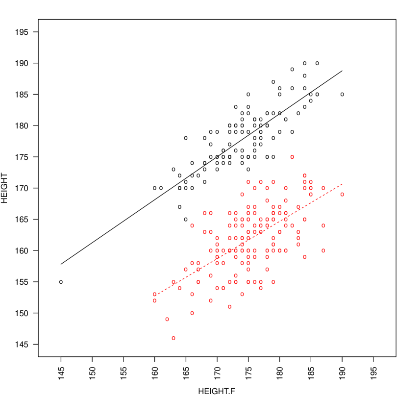
(a) Gaussian CWM

(b) Contaminated Gaussian CWM

Figure 4: Perturbed Student data: scatter plots, labels, and regression lines from the Gaussian CWM (on the left) and from the contaminated Gaussian CWM (on the right; X indicates a detected local good leverage point).

To complete the analysis for the contaminated Gaussian CWM, Table 6 shows the estimated values of the degrees of contamination $\eta_{\mathsf{HEIGHT.F}}$ and $\eta_{\mathsf{HEIGHT}}$ in the group containing the atypical point.

Table 6: Values of the degrees of contamination $\left(\eta_{\mathsf{HEIGHT.F}},\eta_{\mathsf{HEIGHT}}\right)$, for each perturbed data set, in the component of the contaminated Gaussian CWM containing the atypical observation.

	HEIGHT.F
HEIGHT	145	150	155	160	165
195	$\left(10.083,93.845\right)$	$\left(4.637,74,335\right)$	$\left(1.529,57.424\right)$	$\left(1.019,43.559\right)$	$\left(1.005,32.226\right)$
185	$\left(10.087,43.225\right)$	$\left(4.632,31.968\right)$	$\left(1.502,22.836\right)$	$\left(1.004,15.125\right)$
175	$\left(10.070,14.562\right)$	$\left(4.650,\ \ 7.119\right)$	$\left(1.654,\ \ 2.419\right)$
165	$\left(10.132,\ \ 1.086\right)$	$\left(4.652,\ \ 1.000\right)$
155	$\left(10.073,\ \ 1.089\right)$

As expected, the estimate of $\eta_{\mathsf{HEIGHT.F}}$ increases as the value of HEIGHT.F, for the atypical point, further departs from the bulk of the values of HEIGHT.F in its group of membership, regardless from the value of HEIGHT; this can be easily noted by looking at Table 6 column-by-column. Finally, the estimate of $\eta_{\mathsf{HEIGHT}}$ increases as the atypical point further departs from the regression line of the group the atypical point is assigned.

7.2.2 Adding uniform noise

The second sensitivity analysis aims to evaluate the impact of noise on fitting and clustering from the Gaussian CWM and the contaminated Gaussian CWM. With this end, we modify the original data by including twenty noisy points generated from a uniform distribution over a square centered on the bivariate mean $\left(174.963,168.652\right)$ of the observations and with side of length $60$ (centimeters). This square contains the original data. Figure 5 shows the modified data set with bullets denoting uniform noise points.

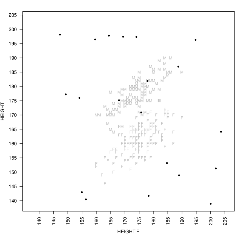
Figure 5: Scatter plot of the Student data where the added uniform noise points are denoted by $\bullet$.

Table 7 shows the BIC values, in correspondence of $k\in\left\{1,2,3\right\}$, for the Gaussian CWM and the contaminated Gaussian CWM.

Table 7: BIC values on the data with uniform noise.

	Gaussian CWM	contaminated Gaussian CWM
$k=1$	-4206.043	-4228.757
$k=2$	-4178.727	-4142.435
$k=3$	-4209.625	-4152.590

Generally, the best model is the contaminated Gaussian CWM with $k=2$. Among the fitted Gaussian CWMs, the best one, in terms of BIC, has $k=2$ components. For comparison’s sake, these models are displayed in Figure 6.

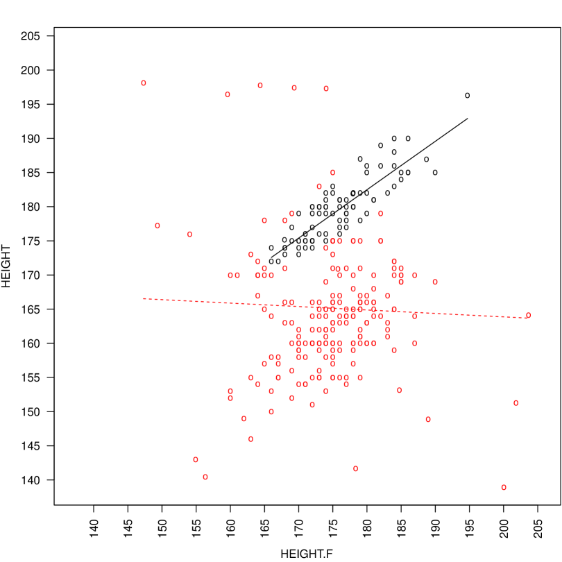
(a) Gaussian CWM

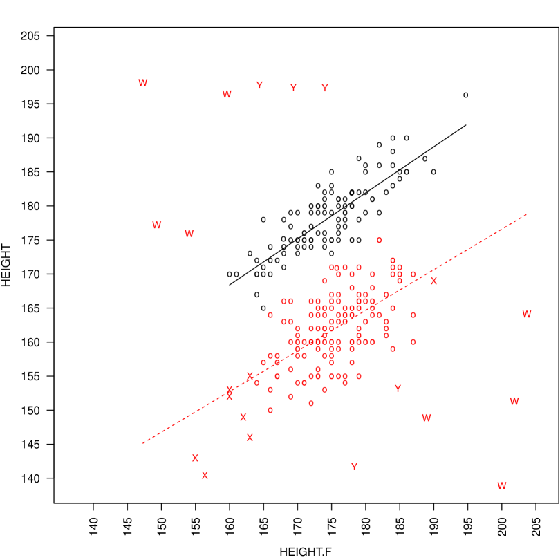
(b) Contaminated Gaussian CWM

Figure 6: Student data with noise: scatter plots, labels, and regression lines from the Gaussian CWM (on the left) and from the contaminated Gaussian CWM (on the right; W denotes bad leverage points, X denotes good leverage points, and Y denotes outliers).

It is important to note that, in Figure 6(b), Y denotes the detected outliers, X indicates the detected good leverage points, and W denotes the bad leverage points. Still importantly, we can see the poor results obtained by the Gaussian CWM, where the regression line referred to the females is severely affected by the noisy observations; as a by-product in clustering terms, the number of original observations misclassified increases from 6 — obtained by the model on the original data only — to 36. On the contrary, our model maintains at 6 the number of misclassified original observations and provides regression lines which are in agreement with those displayed in Figure 1(b). Finally, our model is able to classify each observation, with respect to its group of membership, in accordance to the four categories given in Table 1.

8 Discussion

The contaminated Gaussian CWM has been introduced as a generalization of the Gaussian CWM (Dang et al., 2014) that accommodates atypical observations; the analyses of Section 7 have shown its usefulness. More importantly, however, the contaminated Gaussian CWM is put forward as a gold standard for robust clustering in regression analysis, where observations, in addition to be assigned to the groups, also need to be classified in one of the four categories given in Table 1. Although approaches such as mixtures of $t$ regression models, mixtures of Laplace regression models, and $t$ CWMs, can be used for robust clustering in regression analysis, they assimilate atypical points into clusters rather than separating them out in a direct way. Clusterwise linear regression through trimming can also be used, but it requires a priori specification of the proportion of outliers and leverage points, but this is not always possible in practice; in fact, it is all but impossible if the data cannot easily be visualized.

Another distinct advantage of our contaminated Gaussian CWM over clusterwise linear regression through trimming is that we can easily extend the approach to model-based classification (see, e.g., McNicholas, 2010) and model-based discriminant analysis (Hastie and Tibshirani, 1996). In fact, there are a number of options for the type of supervision that could be used in partial classification applications for our model, i.e., one could specify some of the $\boldsymbol{z}_{i}$ and/or some of the $\boldsymbol{u}_{i}$ and $\boldsymbol{v}_{i}$ a priori, $i=1,\ldots,n$. This provides yet more flexibility than exhibited by any competing approach, as does the ability of our approach to work in higher dimensions where atypical observations cannot easily be visualized.

Future work will focus on the following avenues.

• The development of an R package to facilitate dissemination of our contaminated Gaussian CWM.

• It would be interesting to investigate the sample breakdown points for the proposed method. However, we should note that the analysis of breakdown point for traditional linear regression cannot be directly applied to mixtures of regression models. García-Escudero et al. (2010) also stated that the traditional definition of breakdown point is not the right one to quantify the robustness of mixtures of regression models to atypical observations, since the robustness of these procedures is not only data dependent but also cluster dependent. Hennig (2004) provided a new definition of breakdown points for mixture models based on the breakdown of at least one of the mixture components. Based on the results of Hennig (2004) about mixtures of $t$ distributions, we guess that only extreme outliers would lead to the breakdown of the contaminated Gaussian CWM. Therefore, we believe that the model can still be used as a robust approach with the exception of extreme atypical observations that, however, can easily be deleted.

• In the fashion of Banfield and Raftery (1993) and Celeux and Govaert (1995), and more directly according to Punzo and McNicholas (2014a) and Dang et al. (2014), the proposed approach could be made more flexible and parsimonious by imposing constraints on the eigen-decomposed component matrices $\boldsymbol{\Sigma}_{\boldsymbol{X}|j}$ and $\boldsymbol{\Sigma}_{\boldsymbol{Y}|j}$, $j=1,\ldots,k$. In the fashion of Subedi et al. (2013, 2014) and Punzo and McNicholas (2014b), parsimony, but also dimension reduction, could be obtained by exploiting local factor analyzers.

• Further developments of our model could be obtained by studying the asymptotic properties of the ML estimators and by defining statistical tests for evaluating the significance of the regression coefficients $\boldsymbol{\beta}_{j}$, $j=1,\ldots,k$. Moreover, still working on the eigen-decomposed component matrices $\boldsymbol{\Sigma}_{\boldsymbol{X}|j}$ and $\boldsymbol{\Sigma}_{\boldsymbol{Y}|j}$, $j=1,\ldots,k$, in the fashion of Ingrassia (2004), Ingrassia and Rocci (2007), and Browne et al. (2013), suitable constraints on their eigenvalues during the ECM algorithm could attenuate possible problems on the likelihood function such as unboundedness and spurious local maxima (see also Seo and Kim, 2012).

Appendix A Proof of Proposition 1

Proof. Under the assumptions of the proposition, model (9) simplifies as

$$p\left(\boldsymbol{y}|\boldsymbol{x};\boldsymbol{\vartheta}\right)= \sum_{j=1}^{k}\frac{\pi_{j}f\left(\boldsymbol{x};\boldsymbol{\mu}_{\boldsymbol{X}},\boldsymbol{\Sigma}_{\boldsymbol{X}},\alpha_{\boldsymbol{X}},\eta_{\boldsymbol{X}}\right)}{\displaystyle\sum_{h=1}^{k}\pi_{h}f\left(\boldsymbol{x};\boldsymbol{\mu}_{\boldsymbol{X}},\boldsymbol{\Sigma}_{\boldsymbol{X}},\alpha_{\boldsymbol{X}},\eta_{\boldsymbol{X}}\right)}f\left(\boldsymbol{y};\boldsymbol{\mu}_{\boldsymbol{Y}}\left(\boldsymbol{x};\boldsymbol{\beta}_{j}\right),\boldsymbol{\Sigma}_{\boldsymbol{Y}|j},\alpha_{\boldsymbol{Y}|j},\eta_{\boldsymbol{Y}|j}\right)$$

$$= \sum_{j=1}^{k}\pi_{j}f\left(\boldsymbol{y};\boldsymbol{\mu}_{\boldsymbol{Y}}\left(\boldsymbol{x};\boldsymbol{\beta}_{j}\right),\boldsymbol{\Sigma}_{\boldsymbol{Y}|j},\alpha_{\boldsymbol{Y}|j},\eta_{\boldsymbol{Y}|j}\right),$$

which corresponds to the conditional distribution from a mixture of contaminated Gaussian regression models as defined by (4). ∎

Appendix B Proof of Proposition 2

Proof. Suppose that

$$p\left(\boldsymbol{x},\boldsymbol{y};\boldsymbol{\vartheta}\right)=p\left(\boldsymbol{x},\boldsymbol{y};\widetilde{\boldsymbol{\vartheta}}\right).$$ (26)

Integrating out $\boldsymbol{y}$ from (26) yields

$$\sum_{j=1}^{k}\pi_{j}f\left(\boldsymbol{x};\boldsymbol{\mu}_{\boldsymbol{X}|j},\boldsymbol{\Sigma}_{\boldsymbol{X}|j},\alpha_{\boldsymbol{X}|j},\eta_{\boldsymbol{X}|j}\right)\\ =\sum_{s=1}^{\widetilde{k}}\widetilde{\pi}_{s}f\left(\boldsymbol{x};\widetilde{\boldsymbol{\mu}}_{\boldsymbol{X}|s},\widetilde{\boldsymbol{\Sigma}}_{\boldsymbol{X}|s},\widetilde{\alpha}_{\boldsymbol{X}|s},\widetilde{\eta}_{\boldsymbol{X}|s}\right),$$

corresponding to the marginal distribution of $\boldsymbol{X}$, say $p\left(\boldsymbol{x};\boldsymbol{\pi},\boldsymbol{\mu}_{\boldsymbol{X}},\boldsymbol{\Sigma}_{\boldsymbol{X}},\boldsymbol{\alpha}_{\boldsymbol{X}},\boldsymbol{\eta}_{\boldsymbol{X}}\right)$. Dividing (26) by the left-hand side of (B) leads to

$$p\left(\boldsymbol{y}|\boldsymbol{x};\boldsymbol{\vartheta}\right) =\sum_{j=1}^{k}\frac{\pi_{j}f\left(\boldsymbol{x};\boldsymbol{\mu}_{\boldsymbol{X}|j},\boldsymbol{\Sigma}_{\boldsymbol{X}|j},\alpha_{\boldsymbol{X}|j},\eta_{\boldsymbol{X}|j}\right)}{\displaystyle\sum_{t=1}^{k}\pi_{t}f\left(\boldsymbol{x};\boldsymbol{\mu}_{\boldsymbol{X}|t},\boldsymbol{\Sigma}_{\boldsymbol{X}|t},\alpha_{\boldsymbol{X}|t},\eta_{\boldsymbol{X}|t}\right)}f\left(\boldsymbol{y};\boldsymbol{\mu}_{\boldsymbol{Y}}\left(\boldsymbol{x};\boldsymbol{\beta}_{j}\right),\boldsymbol{\Sigma}_{\boldsymbol{Y}|j},\alpha_{\boldsymbol{Y}|j},\eta_{\boldsymbol{Y}|j}\right)$$

$$=\sum_{s=1}^{\widetilde{k}}\frac{\widetilde{\pi}_{s}f\left(\boldsymbol{x};\widetilde{\boldsymbol{\mu}}_{\boldsymbol{X}|s},\widetilde{\boldsymbol{\Sigma}}_{\boldsymbol{X}|s},\widetilde{\alpha}_{\boldsymbol{X}|s},\widetilde{\eta}_{\boldsymbol{X}|s}\right)}{\displaystyle\sum_{t=1}^{k}\pi_{t}f\left(\boldsymbol{x};\boldsymbol{\mu}_{\boldsymbol{X}|t},\boldsymbol{\Sigma}_{\boldsymbol{X}|t},\alpha_{\boldsymbol{X}|t},\eta_{\boldsymbol{X}|t}\right)}f\left(\boldsymbol{y};\boldsymbol{\mu}_{\boldsymbol{Y}}\left(\boldsymbol{x};\widetilde{\boldsymbol{\beta}}_{s}\right),\widetilde{\boldsymbol{\Sigma}}_{\boldsymbol{Y}|s},\widetilde{\alpha}_{\boldsymbol{Y}|s},\widetilde{\eta}_{\boldsymbol{Y}|s}\right)=p\left(\boldsymbol{y}|\boldsymbol{x};\widetilde{\boldsymbol{\vartheta}}\right).$$ (27)

For each fixed $\boldsymbol{x}$, this is a mixture of contaminated Gaussian distributions for $\boldsymbol{Y}$ (cf. Punzo and McNicholas, 2014a).

Following the scheme of Hennig (2000, p. 292), define the set of all covariate points $\boldsymbol{x}$ which can be used to distinct different regression coefficients $\boldsymbol{\beta}_{j}$ by different values of $\boldsymbol{\mu}_{\boldsymbol{Y}}\left(\boldsymbol{x};\boldsymbol{\beta}_{j}\right)$:

$$\mathcal{X}=\Big{\{}\boldsymbol{x}\in^{d_{\boldsymbol{X}}}:\ \forall\ j,l\in\left\{1,\ldots,k\right\}\text{ and }s,t\in\left\{1,\ldots,\widetilde{k}\right\},$$

$$\boldsymbol{\mu}_{\boldsymbol{Y}}\left(\boldsymbol{x};\boldsymbol{\beta}_{j}\right)=\boldsymbol{\mu}_{\boldsymbol{Y}}\left(\boldsymbol{x};\boldsymbol{\beta}_{l}\right)\ \Rightarrow\ \boldsymbol{\beta}_{j}=\boldsymbol{\beta}_{l},$$

$$\boldsymbol{\mu}_{\boldsymbol{Y}}\left(\boldsymbol{x};\boldsymbol{\beta}_{j}\right)=\boldsymbol{\mu}_{\boldsymbol{Y}}\left(\boldsymbol{x};\widetilde{\boldsymbol{\beta}}_{s}\right)\ \Rightarrow\ \boldsymbol{\beta}_{j}=\widetilde{\boldsymbol{\beta}}_{s},$$

$$\boldsymbol{\mu}_{\boldsymbol{Y}}\left(\boldsymbol{x};\widetilde{\boldsymbol{\beta}}_{s}\right)=\boldsymbol{\mu}_{\boldsymbol{Y}}\left(\boldsymbol{x};\widetilde{\boldsymbol{\beta}}_{t}\right)\ \Rightarrow\ \widetilde{\boldsymbol{\beta}}_{s}=\widetilde{\boldsymbol{\beta}}_{t}\Big{\}}.$$

Note that, $\mathcal{X}$ is complement of a finite union of hyperplanes of ${}^{d_{\boldsymbol{X}}}$. Therefore,

$$\int_{\mathcal{X}}p\left(\boldsymbol{x};\boldsymbol{\pi},\boldsymbol{\mu}_{\boldsymbol{X}},\boldsymbol{\Sigma}_{\boldsymbol{X}},\boldsymbol{\alpha}_{\boldsymbol{X}},\boldsymbol{\eta}_{\boldsymbol{X}}\right)d\boldsymbol{x}=1.$$

For $\boldsymbol{x}\in\mathcal{X}$, all pairs $\left(\boldsymbol{\mu}_{\boldsymbol{Y}}\left(\boldsymbol{x};\boldsymbol{\beta}_{j}\right),\boldsymbol{\Sigma}_{\boldsymbol{Y}|j}\right)$, $j=1,\ldots,k$, are pairwise distinct, because all $\left(\boldsymbol{\beta}_{j},\boldsymbol{\Sigma}_{\boldsymbol{Y}|j}\right)$, $j=1,\ldots,k$, are pairwise distinct for the condition (10) of the proposition. Based on Punzo and McNicholas (2014a), such a condition also guarantees that, for each $\boldsymbol{x}\in\mathcal{X}$, model (27) is identifiable and this implies that $k=\widetilde{k}$ and also implies that for each $j\in\left\{1,\ldots,k\right\}$ there exists an $s\in\left\{1,\ldots,k\right\}$ such that

$$\alpha_{\boldsymbol{Y}|j}=\widetilde{\alpha}_{\boldsymbol{Y}|s},\quad\boldsymbol{\beta}_{j}=\widetilde{\boldsymbol{\beta}}_{s},\quad\boldsymbol{\Sigma}_{\boldsymbol{Y}|j}=\widetilde{\boldsymbol{\Sigma}}_{\boldsymbol{Y}|s},\quad\eta_{\boldsymbol{Y}|j}=\widetilde{\eta}_{\boldsymbol{Y}|s}$$

and

$$\frac{\pi_{j}f\left(\boldsymbol{x};\boldsymbol{\mu}_{\boldsymbol{X}|j},\boldsymbol{\Sigma}_{\boldsymbol{X}|j},\alpha_{\boldsymbol{X}|j},\eta_{\boldsymbol{X}|j}\right)}{\displaystyle\sum_{t=1}^{k}\pi_{t}f\left(\boldsymbol{x};\boldsymbol{\mu}_{\boldsymbol{X}|t},\boldsymbol{\Sigma}_{\boldsymbol{X}|t},\alpha_{\boldsymbol{X}|t},\eta_{\boldsymbol{X}|t}\right)}=\frac{\widetilde{\pi}_{s}f\left(\boldsymbol{x};\widetilde{\boldsymbol{\mu}}_{\boldsymbol{X}|s},\widetilde{\boldsymbol{\Sigma}}_{\boldsymbol{X}|s},\widetilde{\alpha}_{\boldsymbol{X}|s},\widetilde{\eta}_{\boldsymbol{X}|s}\right)}{\displaystyle\sum_{t=1}^{k}\pi_{t}f\left(\boldsymbol{x};\boldsymbol{\mu}_{\boldsymbol{X}|t},\boldsymbol{\Sigma}_{\boldsymbol{X}|t},\alpha_{\boldsymbol{X}|t},\eta_{\boldsymbol{X}|t}\right)}.$$ (28)

Now, based on (26), the equality in (28) simplifies as

$$\pi_{j}f\left(\boldsymbol{x};\boldsymbol{\mu}_{\boldsymbol{X}|j},\boldsymbol{\Sigma}_{\boldsymbol{X}|j},\alpha_{\boldsymbol{X}|j},\eta_{\boldsymbol{X}|j}\right)=\widetilde{\pi}_{s}f\left(\boldsymbol{x};\widetilde{\boldsymbol{\mu}}_{\boldsymbol{X}|s},\widetilde{\boldsymbol{\Sigma}}_{\boldsymbol{X}|s},\widetilde{\alpha}_{\boldsymbol{X}|s},\widetilde{\eta}_{\boldsymbol{X}|s}\right),\quad\forall\ \boldsymbol{x}\in\mathcal{X}.$$ (29)

Integrating (29) over $\boldsymbol{x}\in\mathcal{X}$ yields $\pi_{j}=\widetilde{\pi}_{s}$. Therefore, condition (29) further simplifies as

$$f\left(\boldsymbol{x};\boldsymbol{\mu}_{\boldsymbol{X}|j},\boldsymbol{\Sigma}_{\boldsymbol{X}|j},\alpha_{\boldsymbol{X}|j},\eta_{\boldsymbol{X}|j}\right)=f\left(\boldsymbol{x};\widetilde{\boldsymbol{\mu}}_{\boldsymbol{X}|s},\widetilde{\boldsymbol{\Sigma}}_{\boldsymbol{X}|s},\widetilde{\alpha}_{\boldsymbol{X}|s},\widetilde{\eta}_{\boldsymbol{X}|s}\right),\quad\forall\ \boldsymbol{x}\in\mathcal{X}.$$

The equalities $\alpha_{\boldsymbol{X}|j}=\widetilde{\alpha}_{\boldsymbol{X}|s}$, $\boldsymbol{\mu}_{\boldsymbol{X}|j}=\widetilde{\boldsymbol{\mu}}_{\boldsymbol{X}|s}$, $\boldsymbol{\Sigma}_{\boldsymbol{X}|j}=\widetilde{\boldsymbol{\Sigma}}_{\boldsymbol{X}|s}$, and $\eta_{\boldsymbol{X}|j}=\widetilde{\eta}_{\boldsymbol{X}|s}$ simply arise from the identifiability of the contaminated Gaussian distribution, and this completes the proof. ∎

Appendix C Updates in the first CM-step

The estimates of $\pi_{j}$, $\mu_{\boldsymbol{X}|j}$, $\boldsymbol{\Sigma}_{\boldsymbol{X}|j}$, $\alpha_{\boldsymbol{X}|j}$, $\boldsymbol{\beta}_{j}$, $\boldsymbol{\Sigma}_{\boldsymbol{Y}|j}$, and $\alpha_{\boldsymbol{Y}|j}$, $j=1,\ldots,k$, at the $\left(r+1\right)$th first CM-step of the ECM algorithm, require the maximization of

$$Q\left(\boldsymbol{\vartheta}_{1}|\boldsymbol{\vartheta}^{\left(r\right)}\right)=Q_{1}\left(\boldsymbol{\pi}|\boldsymbol{\vartheta}^{\left(r\right)}\right)+Q_{2}\left(\boldsymbol{\alpha}_{\boldsymbol{X}}|\boldsymbol{\vartheta}^{\left(r\right)}\right)+Q_{3}\left(\boldsymbol{\mu}_{\boldsymbol{X}},\boldsymbol{\Sigma}_{\boldsymbol{X}}|\boldsymbol{\vartheta}^{\left(r\right)}\right)+Q_{4}\left(\boldsymbol{\alpha}_{\boldsymbol{Y}}|\boldsymbol{\vartheta}^{\left(r\right)}\right)+Q_{5}\left(\boldsymbol{\beta},\boldsymbol{\Sigma}_{\boldsymbol{Y}}|\boldsymbol{\vartheta}^{\left(r\right)}\right),$$ (30)

where

$$Q_{1}\left(\boldsymbol{\pi}|\boldsymbol{\vartheta}^{\left(r\right)}\right)=\sum_{i=1}^{n}\sum_{j=1}^{k}z_{ij}^{\left(r\right)}\ln\pi_{j},\qquad\qquad Q_{2}\left(\boldsymbol{\alpha}_{\boldsymbol{X}}|\boldsymbol{\vartheta}^{\left(r\right)}\right)=\sum_{i=1}^{n}\sum_{j=1}^{k}z_{ij}^{\left(r\right)}\left[v_{ij}^{\left(r\right)}\ln\alpha_{\boldsymbol{X}|j}+\left(1-v_{ij}^{\left(r\right)}\right)\ln\left(1-\alpha_{\boldsymbol{X}|j}\right)\right],$$

$$Q_{3}\left(\boldsymbol{\mu}_{\boldsymbol{X}},\boldsymbol{\Sigma}_{\boldsymbol{X}}|\boldsymbol{\vartheta}^{\left(r\right)}\right)=-\frac{1}{2}\sum_{i=1}^{n}\sum_{j=1}^{k}\Biggl{\{}z_{ij}^{\left(r\right)}\ln\left|\boldsymbol{\Sigma}_{\boldsymbol{X}|j}\right|+z_{ij}^{\left(r\right)}\left(v_{ij}^{\left(r\right)}+\frac{1-v_{ij}^{\left(r\right)}}{\eta_{\boldsymbol{X}|j}^{\left(r\right)}}\right)\delta\left(\boldsymbol{x}_{i},\boldsymbol{\mu}_{\boldsymbol{X}|j};\boldsymbol{\Sigma}_{\boldsymbol{X}|j}\right)\Biggr{\}},$$

$$Q_{4}\left(\boldsymbol{\alpha}_{\boldsymbol{Y}}|\boldsymbol{\vartheta}^{\left(r\right)}\right)=\sum_{i=1}^{n}\sum_{j=1}^{k}z_{ij}^{\left(r\right)}\left[u_{ij}^{\left(r\right)}\ln\alpha_{\boldsymbol{Y}|j}+\left(1-u_{ij}^{\left(r\right)}\right)\ln\left(1-\alpha_{\boldsymbol{Y}|j}\right)\right],$$

$$Q_{5}\left(\boldsymbol{\beta},\boldsymbol{\Sigma}_{\boldsymbol{Y}}|\boldsymbol{\vartheta}^{\left(r\right)}\right)=-\frac{1}{2}\sum_{i=1}^{n}\sum_{j=1}^{k}\Biggl{\{}z_{ij}^{\left(r\right)}\ln\left|\boldsymbol{\Sigma}_{\boldsymbol{Y}|j}\right|+z_{ij}^{\left(r\right)}\left(u_{ij}^{\left(r\right)}+\frac{1-u_{ij}^{\left(r\right)}}{\eta_{\boldsymbol{Y}|j}^{\left(r\right)}}\right)\delta\left(\boldsymbol{x}_{i},\boldsymbol{\mu}_{\boldsymbol{Y}}\left(\boldsymbol{x}_{i};\boldsymbol{\beta}_{j}\right);\boldsymbol{\Sigma}_{\boldsymbol{Y}|j}\right)\Biggr{\}}.$$

Terms which are independent by the parameters of interest have been removed from $Q_{3}$ and $Q_{5}$. As the five terms on the right-hand side of (30) have zero cross-derivatives, they can be maximized separately.

C.1 Update of $\boldsymbol{\pi}$

The maximum of $Q_{1}\left(\boldsymbol{\pi}|\boldsymbol{\vartheta}^{\left(r\right)}\right)$ with respect to $\boldsymbol{\pi}$, subject to the constraints on those parameters, is obtained by maximizing the augmented function

$$\sum_{i=1}^{n}\sum_{j=1}^{k}z_{ij}^{\left(r\right)}\ln\pi_{j}-\lambda\left(\sum_{j=1}^{k}\pi_{j}-1\right),$$ (31)

where $\lambda$ is a Lagrangian multiplier. Setting the derivative of equation (31) with respect to $\pi_{j}$ equal to zero and solving for $\pi_{j}$ yields

$$\pi_{j}^{\left(r+1\right)}=\displaystyle\displaystyle\sum_{i=1}^{n}z_{ij}^{\left(r\right)}\Big{/}n.$$

C.2 Update of $\boldsymbol{\alpha}_{\boldsymbol{X}}$

The updates for $\boldsymbol{\alpha}_{\boldsymbol{X}}$ can be obtained through the first partial derivatives

$$\frac{\partial Q_{2}\left(\boldsymbol{\alpha}_{\boldsymbol{X}}|\boldsymbol{\vartheta}^{\left(r\right)}\right)}{\partial\alpha_{\boldsymbol{X}|j}} =\frac{1}{\alpha_{\boldsymbol{X}|j}}\sum_{i=1}^{n}z_{ij}^{\left(r\right)}v_{ij}^{\left(r\right)}-\frac{1}{1-\alpha_{\boldsymbol{X}|j}}\sum_{i=1}^{n}z_{ij}^{\left(r\right)}\left(1-v_{ij}^{\left(r\right)}\right)=\frac{\displaystyle\sum_{i=1}^{n}z_{ij}^{\left(r\right)}v_{ij}^{\left(r\right)}-\alpha_{\boldsymbol{X}|j}\sum_{i=1}^{n}z_{ij}^{\left(r\right)}}{\alpha_{\boldsymbol{X}|j}\left(1-\alpha_{\boldsymbol{X}|j}\right)},\qquad j=1,\ldots,k.$$ (32)

Equating (32) to zero yields

$$\alpha_{\boldsymbol{X}|j}^{\left(r+1\right)}=\displaystyle\sum_{i=1}^{n}z_{ij}^{\left(r\right)}v_{ij}^{\left(r\right)}\Bigg{/}\displaystyle\sum_{i=1}^{n}z_{ij}^{\left(r\right)},\qquad j=1,\ldots,k.$$

C.3 Update of $\boldsymbol{\mu}_{\boldsymbol{X}}$ and $\boldsymbol{\Sigma}_{\boldsymbol{X}}$

The updates for $\boldsymbol{\mu}_{\boldsymbol{X}}$ can be obtained through the first partial derivatives

$$\frac{\partial Q_{3}\left(\boldsymbol{\mu}_{\boldsymbol{X}},\boldsymbol{\Sigma}_{\boldsymbol{X}}|\boldsymbol{\vartheta}^{\left(r\right)}\right)}{\partial\boldsymbol{\mu}_{\boldsymbol{X}|j}} =\frac{\partial\left[-\displaystyle\frac{1}{2}\displaystyle\sum_{i=1}^{n}z_{ij}^{\left(r\right)}\left(v_{ij}^{\left(r\right)}+\frac{1-v_{ij}^{\left(r\right)}}{\eta_{\boldsymbol{X}|j}^{\left(r\right)}}\right)\left(\boldsymbol{x}_{i}-\boldsymbol{\mu}_{\boldsymbol{X}|j}\right)^{\prime}\boldsymbol{\Sigma}_{\boldsymbol{X}|j}^{-1}\left(\boldsymbol{x}_{i}-\boldsymbol{\mu}_{\boldsymbol{X}|j}\right)\right]}{\partial\boldsymbol{\mu}_{\boldsymbol{X}|j}}$$

$$=\sum_{i=1}^{n}z_{ij}^{\left(r\right)}\left(v_{ij}^{\left(r\right)}+\frac{1-v_{ij}^{\left(r\right)}}{\eta_{\boldsymbol{X}|j}^{\left(r\right)}}\right)\boldsymbol{\Sigma}_{\boldsymbol{X}|j}^{-1}\left(\boldsymbol{x}_{i}-\boldsymbol{\mu}_{\boldsymbol{X}|j}\right),\qquad j=1,\ldots,k.$$ (33)

Equating (33) to the null vector yields

$$\boldsymbol{\mu}_{\boldsymbol{X}|j}^{\left(r+1\right)}=\sum_{i=1}^{n}\frac{z_{ij}^{\left(r\right)}\displaystyle\left(v_{ij}^{\left(r\right)}+\frac{1-v_{ij}^{\left(r\right)}}{\eta_{\boldsymbol{X}|j}^{\left(r\right)}}\right)}{\displaystyle\sum_{q=1}^{n}{z}_{qj}^{\left(r\right)}\left(v_{qj}^{\left(r\right)}+\frac{1-v_{qj}^{\left(r\right)}}{\eta_{\boldsymbol{X}|j}^{\left(r\right)}}\right)}\boldsymbol{x}_{i},\qquad j=1,\ldots,k.$$

The updates for $\boldsymbol{\Sigma}_{\boldsymbol{X}}$, using results from matrix derivatives and trace operator (see, e.g., Lütkepohl, 1996), can be obtained through the first partial derivatives

$$\frac{\partial Q_{3}\left(\boldsymbol{\mu}_{\boldsymbol{X}},\boldsymbol{\Sigma}_{\boldsymbol{X}}|\boldsymbol{\vartheta}^{\left(r\right)}\right)}{\partial\boldsymbol{\Sigma}_{\boldsymbol{X}|j}^{-1}} =\frac{\partial\left\{\displaystyle\frac{1}{2}\displaystyle\sum_{i=1}^{n}z_{ij}^{\left(r\right)}\left\{\ln\left|\boldsymbol{\Sigma}_{\boldsymbol{X}|j}^{-1}\right|-\left(v_{ij}^{\left(r\right)}+\displaystyle\frac{1-v_{ij}^{\left(r\right)}}{\eta_{\boldsymbol{X}|j}^{\left(r\right)}}\right)\operatorname{\text{tr}}\left[\left(\boldsymbol{x}_{i}-\boldsymbol{\mu}_{\boldsymbol{X}|j}^{\left(r+1\right)}\right)^{\prime}\boldsymbol{\Sigma}_{\boldsymbol{X}|j}^{-1}\left(\boldsymbol{x}_{i}-\boldsymbol{\mu}_{\boldsymbol{X}|j}^{\left(r+1\right)}\right)\right]\right\}\right\}}{\partial\boldsymbol{\Sigma}_{\boldsymbol{X}|j}^{-1}}$$

$$=\frac{\partial\left\{\displaystyle\frac{1}{2}\displaystyle\sum_{i=1}^{n}z_{ij}^{\left(r\right)}\left\{\ln\left|\boldsymbol{\Sigma}_{\boldsymbol{X}|j}^{-1}\right|-\left(v_{ij}^{\left(r\right)}+\displaystyle\frac{1-v_{ij}^{\left(r\right)}}{\eta_{\boldsymbol{X}|j}^{\left(r\right)}}\right)\operatorname{\text{tr}}\left[\boldsymbol{\Sigma}_{\boldsymbol{X}|j}^{-1}\left(\boldsymbol{x}_{i}-\boldsymbol{\mu}_{\boldsymbol{X}|j}^{\left(r+1\right)}\right)\left(\boldsymbol{x}_{i}-\boldsymbol{\mu}_{\boldsymbol{X}|j}^{\left(r+1\right)}\right)^{\prime}\right]\right\}\right\}}{\partial\boldsymbol{\Sigma}_{\boldsymbol{X}|j}^{-1}}$$

$$=\displaystyle\frac{1}{2}\displaystyle\sum_{i=1}^{n}z_{ij}^{\left(r\right)}\left[\boldsymbol{\Sigma}_{\boldsymbol{X}|j}+\left(v_{ij}^{\left(r\right)}+\displaystyle\frac{1-v_{ij}^{\left(r\right)}}{\eta_{\boldsymbol{X}|j}^{\left(r\right)}}\right)\left(\boldsymbol{x}_{i}-\boldsymbol{\mu}_{\boldsymbol{X}|j}^{\left(r+1\right)}\right)\left(\boldsymbol{x}_{i}-\boldsymbol{\mu}_{\boldsymbol{X}|j}^{\left(r+1\right)}\right)^{\prime}\right],\qquad j=1,\ldots,k.$$ (34)

Equating (34) to the null matrix yields

$$\boldsymbol{\Sigma}_{\boldsymbol{X}|j}^{\left(r+1\right)}=\frac{1}{\displaystyle\sum_{i=1}^{n}z_{ij}^{\left(r\right)}}\sum_{i=1}^{n}z_{ij}^{\left(r\right)}\left(v_{ij}^{\left(r\right)}+\frac{1-v_{ij}^{\left(r\right)}}{\eta_{\boldsymbol{X}|j}^{\left(r\right)}}\right)\left(\boldsymbol{x}_{i}-\displaystyle\boldsymbol{\mu}_{\boldsymbol{X}|j}^{\left(r+1\right)}\right)\left(\boldsymbol{x}_{i}-\displaystyle\boldsymbol{\mu}_{\boldsymbol{X}|j}^{\left(r+1\right)}\right)^{\prime},\qquad j=1,\ldots,k.$$

C.4 Update of $\boldsymbol{\alpha}_{\boldsymbol{Y}}$

Analogously to C.2, the updates for $\boldsymbol{\alpha}_{\boldsymbol{Y}}$ can be obtained through the first partial derivatives

$$\frac{\partial Q_{4}\left(\boldsymbol{\alpha}_{\boldsymbol{Y}}|\boldsymbol{\vartheta}^{\left(r\right)}\right)}{\partial\alpha_{\boldsymbol{Y}|j}}=\frac{\displaystyle\sum_{i=1}^{n}z_{ij}^{\left(r\right)}u_{ij}^{\left(r\right)}-\alpha_{\boldsymbol{Y}|j}\sum_{i=1}^{n}z_{ij}^{\left(r\right)}}{\alpha_{\boldsymbol{Y}|j}\left(1-\alpha_{\boldsymbol{Y}|j}\right)},\qquad j=1,\ldots,k.$$ (35)

Equating (35) to zero yields

$$\alpha_{\boldsymbol{Y}|j}^{\left(r+1\right)}=\displaystyle\sum_{i=1}^{n}z_{ij}^{\left(r\right)}u_{ij}^{\left(r\right)}\Bigg{/}\displaystyle\sum_{i=1}^{n}z_{ij}^{\left(r\right)},\qquad j=1,\ldots,k.$$

C.5 Update of $\boldsymbol{\beta}$ and $\boldsymbol{\Sigma}_{\boldsymbol{Y}}$

Using properties of trace and transpose, the updates for $\boldsymbol{\beta}$ can be obtained through the first partial derivatives

$$\frac{\partial Q_{5}\left(\boldsymbol{\beta},\boldsymbol{\Sigma}_{\boldsymbol{Y}}|\boldsymbol{\vartheta}^{\left(r\right)}\right)}{\partial\boldsymbol{\beta}_{j}^{\prime}} =\frac{\partial\left\{-\displaystyle\frac{1}{2}\displaystyle\sum_{i=1}^{n}z_{ij}^{\left(r\right)}\left(u_{ij}^{\left(r\right)}+\frac{1-u_{ij}^{\left(r\right)}}{\eta_{\boldsymbol{Y}|j}^{\left(r\right)}}\right)\left[\boldsymbol{y}_{i}-\boldsymbol{\mu}_{\boldsymbol{Y}}\left(\boldsymbol{x}_{i};\boldsymbol{\beta}_{j}\right)\right]^{\prime}\boldsymbol{\Sigma}_{\boldsymbol{X}|j}^{-1}\left[\boldsymbol{y}_{i}-\boldsymbol{\mu}_{\boldsymbol{Y}}\left(\boldsymbol{x}_{i};\boldsymbol{\beta}_{j}\right)\right]\right\}}{\partial\boldsymbol{\beta}_{j}^{\prime}}$$

$$=\frac{\partial\left[-\displaystyle\frac{1}{2}\displaystyle\sum_{i=1}^{n}z_{ij}^{\left(r\right)}\left(u_{ij}^{\left(r\right)}+\frac{1-u_{ij}^{\left(r\right)}}{\eta_{\boldsymbol{Y}|j}^{\left(r\right)}}\right)\left(-\boldsymbol{y}_{i}^{\prime}\boldsymbol{\Sigma}_{\boldsymbol{Y}|j}^{-1}\boldsymbol{\beta}_{j}^{\prime}\boldsymbol{x}_{i}^{*}-\boldsymbol{x}_{i}^{*^{\prime}}\boldsymbol{\beta}_{j}\boldsymbol{\Sigma}_{\boldsymbol{Y}|j}^{-1}\boldsymbol{y}_{i}+\boldsymbol{x}_{i}^{*^{\prime}}\boldsymbol{\beta}_{j}\boldsymbol{\Sigma}_{\boldsymbol{Y}|j}^{-1}\boldsymbol{\beta}_{j}^{\prime}\boldsymbol{x}_{i}^{*}\right)\right]}{\partial\boldsymbol{\beta}_{j}^{\prime}}$$

$$=\frac{\partial\left\{\displaystyle\frac{1}{2}\displaystyle\sum_{i=1}^{n}z_{ij}^{\left(r\right)}\left(u_{ij}^{\left(r\right)}+\frac{1-u_{ij}^{\left(r\right)}}{\eta_{\boldsymbol{Y}|j}^{\left(r\right)}}\right)\left[\operatorname{\text{tr}}\left(\boldsymbol{\beta}_{j}^{\prime}\boldsymbol{x}_{i}^{*}\boldsymbol{y}_{i}^{\prime}\boldsymbol{\Sigma}_{\boldsymbol{Y}|j}^{-1}\right)+\operatorname{\text{tr}}\left(\left(\boldsymbol{\Sigma}_{\boldsymbol{Y}|j}^{-1}\boldsymbol{y}_{i}\boldsymbol{x}_{i}^{*^{\prime}}\right)^{\prime}\boldsymbol{\beta}_{j}^{\prime}\right)-\operatorname{\text{tr}}\left(\boldsymbol{\beta}_{j}^{\prime}\boldsymbol{x}_{i}^{*}\boldsymbol{x}_{i}^{*^{\prime}}\boldsymbol{\beta}_{j}\boldsymbol{\Sigma}_{\boldsymbol{Y}|j}^{-1}\right)\right]\right\}}{\partial\boldsymbol{\beta}_{j}^{\prime}}$$

$$=\displaystyle\frac{1}{2}\displaystyle\sum_{i=1}^{n}z_{ij}^{\left(r\right)}\left(u_{ij}^{\left(r\right)}+\frac{1-u_{ij}^{\left(r\right)}}{\eta_{\boldsymbol{Y}|j}^{\left(r\right)}}\right)\left(2\boldsymbol{\Sigma}_{\boldsymbol{Y}|j}^{-1}\boldsymbol{y}_{i}\boldsymbol{x}_{i}^{*^{\prime}}-2\boldsymbol{\Sigma}_{\boldsymbol{Y}|j}^{-1}\boldsymbol{\beta}_{j}^{\prime}\boldsymbol{x}_{i}^{*}\boldsymbol{x}_{i}^{*^{\prime}}\right),\qquad j=1,\ldots,k.$$ (36)

Equating (36) to the null matrix yields

$$\boldsymbol{\beta}_{j}^{\left(r+1\right)}=\left[\sum_{i=1}^{n}z_{ij}^{\left(r\right)}\left(u_{ij}^{\left(r\right)}+\frac{1-u_{ij}^{\left(r\right)}}{\eta_{\boldsymbol{Y}|j}^{\left(r\right)}}\right)\boldsymbol{x}_{i}^{*}\boldsymbol{x}_{i}^{*^{\prime}}\right]^{-1}\left[\sum_{i=1}^{n}z_{ij}^{\left(r\right)}\left(u_{ij}^{\left(r\right)}+\frac{1-u_{ij}^{\left(r\right)}}{\eta_{\boldsymbol{Y}|j}^{\left(r\right)}}\right)\boldsymbol{x}_{i}^{*}\boldsymbol{y}_{i}\right],\qquad j=1,\ldots,k.$$

Finally, the updates for $\boldsymbol{\Sigma}_{\boldsymbol{Y}}$ can be obtained, analogously to the updates for $\boldsymbol{\Sigma}_{\boldsymbol{X}}$ given in C.3, through the first partial derivatives

$$\frac{\partial Q_{5}\left(\boldsymbol{\beta},\boldsymbol{\Sigma}_{\boldsymbol{Y}}|\boldsymbol{\vartheta}^{\left(r\right)}\right)}{\partial\boldsymbol{\Sigma}_{\boldsymbol{Y}|j}^{-1}}=\displaystyle\frac{1}{2}\displaystyle\sum_{i=1}^{n}z_{ij}^{\left(r\right)}\left\{\boldsymbol{\Sigma}_{\boldsymbol{Y}|j}+\left(u_{ij}^{\left(r\right)}+\displaystyle\frac{1-u_{ij}^{\left(r\right)}}{\eta_{\boldsymbol{Y}|j}^{\left(r\right)}}\right)\left[\boldsymbol{y}_{i}-\boldsymbol{\mu}_{\boldsymbol{Y}}\left(\boldsymbol{x}_{i};\boldsymbol{\beta}_{j}^{\left(r+1\right)}\right)\right]\left[\boldsymbol{y}_{i}-\boldsymbol{\mu}_{\boldsymbol{Y}}\left(\boldsymbol{x}_{i};\boldsymbol{\beta}_{j}^{\left(r+1\right)}\right)\right]^{\prime}\right\},\qquad j=1,\ldots,k.$$ (37)

Equating (37) to the null matrix yields

$$\boldsymbol{\Sigma}_{\boldsymbol{Y}|j}^{\left(r+1\right)}=\frac{1}{n_{j}^{\left(r\right)}}\sum_{i=1}^{n}z_{ij}^{\left(r\right)}\left(u_{ij}^{\left(r\right)}+\frac{1-u_{ij}^{\left(r\right)}}{\eta_{\boldsymbol{Y}|j}^{\left(r\right)}}\right)\left[\boldsymbol{y}_{i}-\displaystyle\boldsymbol{\mu}_{\boldsymbol{Y}}\left(\boldsymbol{x}_{i};\boldsymbol{\beta}_{j}^{\left(r+1\right)}\right)\right]\left[\boldsymbol{y}_{i}-\displaystyle\boldsymbol{\mu}_{\boldsymbol{Y}}\left(\boldsymbol{x}_{i};\boldsymbol{\beta}_{j}^{\left(r+1\right)}\right)\right]^{\prime},\qquad j=1,\ldots,k.$$

References

References

- Aitken (1926) Aitken, A. C., 1926. On Bernoulli’s numerical solution of algebraic equations. In: Proceedings of the Royal Society of Edinburgh. Vol. 46. pp. 289–305.
- Aitkin and Wilson (1980) Aitkin, M., Wilson, G. T., 1980. Mixture models, outliers, and the EM algorithm. Technometrics 22 (3), 325–331.
- Bagnato and Punzo (2013) Bagnato, L., Punzo, A., 2013. Finite mixtures of unimodal beta and gamma densities and the -bumps algorithm. Computational Statistics 28 (4), 1571–1597.
- Bai et al. (2012) Bai, X., Yao, W., Boyer, J. E., 2012. Robust fitting of mixture regression models. Computational Statistics & Data Analysis 56 (7), 2347–2359.
- Banfield and Raftery (1993) Banfield, J. D., Raftery, A. E., 1993. Model-based Gaussian and non-Gaussian clustering. Biometrics 49 (3), 803–821.
- Berkane and Bentler (1988) Berkane, M., Bentler, P. M., 1988. Estimation of contamination parameters and identification of outliers in multivariate data. Sociological Methods & Research 17 (1), 55–64.
- Biernacki et al. (2003) Biernacki, C., Celeux, G., Govaert, G., 2003. Choosing starting values for the EM algorithm for getting the highest likelihood in multivariate Gaussian mixture models. Computational Statistics & Data Analysis 41 (3-4), 561–575.
- Böhning et al. (1994) Böhning, D., Dietz, E., Schaub, R., Schlattmann, P., Lindsay, B., 1994. The distribution of the likelihood ratio for mixtures of densities from the one-parameter exponential family. Annals of the Institute of Statistical Mathematics 46 (2), 373–388.
- Browne et al. (2013) Browne, R. P., Subedi, S., McNicholas, P. D., 2013. Constrained optimization for a subset of the Gaussian parsimonious clustering models. arXiv.org e-print 1306.5824, available at: http://arxiv.org/abs/1306.5824.
- Celeux and Govaert (1995) Celeux, G., Govaert, G., 1995. Gaussian parsimonious clustering models. Pattern Recognition 28 (5), 781–793.
- Celeux et al. (2000) Celeux, G., Hurn, M., Robert, C. P., 2000. Computational and inferential difficulties with mixture posterior distributions. Journal of the American Statistical Association 95 (451), 957–970.
- Dang et al. (2014) Dang, U. J., Punzo, A., McNicholas, P. D., Ingrassia, S., Browne, R. P., 2014. Multivariate response and parsimony for Gaussian cluster-weighted models, manuscript in preparation.
- Davies and Gather (1993) Davies, L., Gather, U., 1993. The identification of multiple outliers. Journal of the American Statistical Association 88 (423), 782–792.
- Dempster et al. (1977) Dempster, A., Laird, N., Rubin, D., 1977. Maximum likelihood from incomplete data via the EM algorithm. Journal of the Royal Statistical Society. Series B (Methodological) 39 (1), 1–38.
- DeSarbo and Cron (1988) DeSarbo, W. S., Cron, W. L., 1988. A maximum likelihood methodology for clusterwise linear regression. Journal of Classification 5 (2), 249–282.
- Fraley et al. (2012) Fraley, C., Raftery, A. E., Murphy, T. B., Scrucca, L., 2012. mclust version 4 for R: Normal mixture modeling for model-based clustering, classification, and density estimation. Technical report 597, Department of Statistics, University of Washington, Seattle, Washington, USA.
- Frühwirth-Schnatter (2006) Frühwirth-Schnatter, S., 2006. Finite mixture and Markov switching models. Springer, New York.
- Galimberti and Soffritti (2014) Galimberti, G., Soffritti, G., 2014. A multivariate linear regression analysis using finite mixtures of distributions. Computational Statistics & Data Analysis 71, 138–150.
- García-Escudero et al. (2010) García-Escudero, L. A., Gordaliza, A., Mayo-Iscar, A., San Martín, R., 2010. Robust clusterwise linear regression through trimming. Computational Statistics & Data Analysis 54 (12), 3057–3069.
- Gershenfeld (1997) Gershenfeld, N., 1997. Nonlinear inference and cluster-weighted modeling. Annals of the New York Academy of Sciences 808 (1), 18–24.
- Hastie and Tibshirani (1996) Hastie, T., Tibshirani, R., 1996. Discriminant analysis by Gaussian mixtures. Journal of the Royal Statistical Society. Series B (Methodological) 58 (1), 155–176.
- Hennig (2000) Hennig, C., 2000. Identifiablity of models for clusterwise linear regression. Journal of Classification 17 (2), 273–296.
- Hennig (2002) Hennig, C., 2002. Fixed point clusters for linear regression: computation and comparison. Journal of classification 19 (2), 249–276.
- Hennig (2004) Hennig, C., 2004. Breakdown points for maximum likelihood estimators of location-scale mixtures. The Annals of Statistics 32 (4), 1313–1340.
- Ingrassia (2004) Ingrassia, S., 2004. A likelihood-based constrained algorithm for multivariate normal mixture models. Statistical Methods and Applications 13 (2), 151–166.
- Ingrassia et al. (2014) Ingrassia, S., Minotti, S. C., Punzo, A., 2014. Model-based clustering via linear cluster-weighted models. Computational Statistics and Data Analysis 71, 159–182.
- Ingrassia et al. (2012) Ingrassia, S., Minotti, S. C., Vittadini, G., 2012. Local statistical modeling via the cluster-weighted approach with elliptical distributions. Journal of Classification 29 (3), 363–401.
- Ingrassia and Rocci (2007) Ingrassia, S., Rocci, R., 2007. Constrained monotone em algorithms for finite mixture of multivariate Gaussians. Computational Statistics & Data Analysis 51 (11), 5339–5351.
- Karlis and Xekalaki (2003) Karlis, D., Xekalaki, E., 2003. Choosing initial values for the EM algorithm for finite mixtures. Computational Statistics & Data Analysis 41 (3–4), 577–590.
- Kotz and Nadarajah (2004) Kotz, S., Nadarajah, S., 2004. Multivariate -Distributions and Their Applications. Cambridge University Press, Cambridge.
- Lange et al. (1989) Lange, K. L., Little, R. J. A., Taylor, J. M. G., 1989. Robust statistical modeling using the distribution. Journal of the American Statistical Association 84 (408), 881–896.
- Little (1988) Little, R. J. A., 1988. Robust estimation of the mean and covariance matrix from data with missing values. Applied Statistics 37 (1), 23–38.
- Lütkepohl (1996) Lütkepohl, H., 1996. Handbook of Matrices. Wiley, Chicester.
- Mardia et al. (1997) Mardia, K. V., Kent, J. T., Bibby, J. M., 1997. Multivariate Analysis. Probability and Mathematical Statistics. Academic Press, London.
- McLachlan and Krishnan (2007) McLachlan, G., Krishnan, T., 2007. The EM algorithm and extensions, 2nd Edition. Vol. 382 of Wiley Series in Probability and Statistics. John Wiley & Sons, New York.
- McLachlan and Basford (1988) McLachlan, G. J., Basford, K. E., 1988. Mixture models: Inference and Applications to clustering. Marcel Dekker, New York.
- McLachlan and Peel (2000) McLachlan, G. J., Peel, D., 2000. Finite Mixture Models. John Wiley & Sons, New York.
- McNicholas (2010) McNicholas, P. D., 2010. Model-based classification using latent Gaussian mixture models. Journal of Statistical Planning and Inference 140 (5), 1175–1181.
- Meng and Rubin (1993) Meng, X.-L., Rubin, D. B., 1993. Maximum likelihood estimation via the ECM algorithm: A general framework. Biometrika 80 (2), 267–278.
- Neykov et al. (2007) Neykov, N., Filzmoser, P., Dimova, R., Neytchev, P., 2007. Robust fitting of mixtures using the trimmed likelihood estimator. Computational Statistics & Data Analysis 52 (1), 299–308.
- Punzo (2014) Punzo, A., 2014. Flexible mixture modeling with the polynomial Gaussian cluster-weighted model. Statistical Modelling 14 (3), 257–291.
- Punzo and McNicholas (2014a) Punzo, A., McNicholas, P. D., 2014a. Robust clustering via parsimonious mixtures of contaminated Gaussian distributions. arXiv.org e-print 1305.4669, available at: http://arxiv.org/abs/1305.4669.
- Punzo and McNicholas (2014b) Punzo, A., McNicholas, P. D., 2014b. Robust high-dimensional modeling with the contaminated Gaussian distribution. arXiv.org e-print 1408.2128, available at: http://arxiv.org/abs/1408.2128.
-
R Core Team (2013)
R Core Team, 2013. R: A Language and Environment for Statistical
Computing. R Foundation for Statistical Computing, Vienna, Austria.
URL http://www.R-project.org/ - Rousseeuw and Leroy (2005) Rousseeuw, P. J., Leroy, A. M., 2005. Robust Regression and Outlier Detection. Wiley Series in Probability and Statistics. Wiley.
- Rousseeuw and Van Zomeren (1990) Rousseeuw, P. J., Van Zomeren, B. C., 1990. Unmasking multivariate outliers and leverage points. Journal of the American Statistical Association 85 (411), 633–639.
- Schwarz (1978) Schwarz, G., 1978. Estimating the dimension of a model. The Annals of Statistics 6 (2), 461–464.
- Seo and Kim (2012) Seo, B., Kim, D., 2012. Root selection in normal mixture models. Computational Statistics & Data Analysis 56 (8), 2454–2470.
- Song et al. (2014) Song, W., Yao, W., Xing, Y., 2014. Robust mixture regression model fitting by Laplace distribution. Computational Statistics & Data Analysis 71, 128–137.
- Stephens (2000) Stephens, M., 2000. Dealing with label switching in mixture models. Journal of the Royal Statistical Society. Series B: Statistical Methodology 62 (4), 795–809.
- Subedi et al. (2013) Subedi, S., Punzo, A., Ingrassia, S., McNicholas, P. D., 2013. Clustering and classification via cluster-weighted factor analyzers. Advances in Data Analysis and Classification 7 (1), 5–40.
- Subedi et al. (2014) Subedi, S., Punzo, A., Ingrassia, S., McNicholas, P. D., 2014. Cluster-weighted -factor analyzers for robust model-based clustering and dimension reduction. Statistical Methods and Applications (submitted).
- Titterington et al. (1985) Titterington, D. M., Smith, A. F. M., Makov, U. E., 1985. Statistical Analysis of Finite Mixture Distributions. John Wiley & Sons, New York.
- Wedel (2002) Wedel, M., 2002. Concomitant variables in finite mixture models. Statistica Neerlandica 56 (3), 362–375.
- Yao (2012) Yao, W., 2012. Model based labeling for mixture models. Statistics and Computing 22 (2), 337–347.
- Yao et al. (2014) Yao, W., Wei, Y., Yu, C., 2014. Robust mixture regression using the -distribution. Computational Statistics & Data Analysis 71, 116–127.