On the Mean Stability of a Class of Switched Linear Systems

Abstract

This paper investigates the mean stability of a class of discrete-time stochastic switched linear systems using the $L^{p}$-norm joint spectral radius of the probability distributions governing the switched systems. First we prove a converse Lyapunov theorem that shows the equivalence between the mean stability and the existence of a homogeneous Lyapunov function. Then we show that, when $p$ goes to $\infty$, the stability of the $p$th mean becomes equivalent to the absolute asymptotic stability of an associated deterministic switched system. Finally we study the mean stability of Markovian switched systems. Numerical examples are presented to illustrate the results.

I Introduction

This paper studies the discrete-time stochastic switched linear system of the form

$$\Sigma:x(k+1)=A_{k}x(k)$$ (1)

where $x(k)$ represents a finite-dimensional state vector and $\{A_{k}\}_{k=0}^{\infty}$ is a stochastic process taking values in the set of square matrices of an appropriate dimension. One of its most natural stability notions is almost sure stability [16], which requires that the state $x(k)$ converges to the origin with probability one as $k\to\infty$. However this stability is difficult to check in practice because it is characterized by a quantity called the top Lyapunov exponent, whose computation is in general a hard problem [22]. For example, the necessary and sufficient condition in [6] is one of the most tractable conditions but cannot necessarily be checked with finite computation.

This difficulty has motivated many authors to study another stability, called $p$th mean stability, which requires that the expected value of the $p$th power of the norm of the state $x(k)$ converges to $0$. It is well known [14, 10, 11, 12, 24] that the $p$th mean stability can be often checked by computing the spectral radius of a matrix that is easy to compute. Recently the authors showed [18] that, if each $A_{k}$ follows an identical probability distribution independently and either $p$ is even or the distribution possess a certain invariance property, then the $p$th mean stability of the system (1) is characterized by the spectral radius of a matrix, generalizing the results obtained in the literature [14, 10, 11]. Also it is shown that the mean square stability is equivalent to the existence of a certain quadratic Lyapunov function. The derivation of these results depends on an extended version [18] of $L^{p}$-norm joint spectral radius [19].

Generalizing the above result on Lyapunov functions, in this paper we first show that, for a general even exponent $p$, the $p$th mean stability of $\Sigma$ is equivalent to the existence of a homogeneous Lyapunov function of degree $p$. This equivalence is still true for a general $p$ provided the distribution possesses a certain invariance property. Imposing that the value of the function decreases along trajectories only in expectation enables us to construct a Lyapunov function even when the system is not stable for an arbitrary switching signal, as opposed to the results in the literature [17, 7, 8], Moreover our Lyapunov function can be constructed easily by solving a linear matrix inequality or an eigenvalue problem.

Then we study a limiting behavior of the $p$th mean stability. It is well known [9] that, roughly speaking, the $p$th mean stability becomes equivalent to almost sure stability in the limit of $p\to 0$. As a counterpart of this fact we show that, in the limit of $p\to\infty$, the $p$th mean stability is equivalent to the stability of an associated deterministic switched system for an arbitrary switching. This result will be proved by showing an extension of the formulas [2, 25] that express joint spectral radius as the limit of $L^{p}$-norm joint spectral radius.

Finally we extend the results in [18] to Markovian switched systems, where $A_{k}$ in (1) is not necessarily identically and independently distributed. Again assuming the invariantce property of the Markov process we will give a characterization of the $p$th mean stability.

This paper is organized as follows. After preparing necessary mathematical notation and conventions, in Section II we review the basic facts of the stability of discrete-time linear switched systems. Section III proves a converse Lyapunov theorem. Then in Section IV we study the limiting behavior of the $p$th mean stability. Finally Section V studies the mean stability of Markovian switched systems.

I-A Mathematical Preliminaries

Let $\mathbb{R}_{+}$ denote the set of nonnegative numbers. The spectral radius of a square matrix is denoted by $\rho(\cdot)$. A subset $K\subset\mathbb{R}^{d}$ is called a cone if $K$ is closed under multiplication by nonnegative scalars. The cone is said to be solid if it possesses a nonempty interior. We say that a cone is pointed if it contains no line; i.e., if $x,-x\in K$ then $x=0$. We say that $K$ is proper if it is closed, convex, solid, and pointed. For example the positive orthant $\mathbb{R}^{d}_{+}$ of $\mathbb{R}^{d}$ is a proper cone. The dual cone $K^{*}$ is defined by

$$K^{*}=\{f\in\mathbb{R}^{d}:f^{\top}x\geq 0\text{ for every $x\in K$}\}.$$

A matrix $M\in\mathbb{R}^{d\times d}$ is said to leave $K$ invariant, written $M\geq^{K}0$, if $MK\subset K$. A subset $\mathcal{M}\subset\mathbb{R}^{d\times d}$ is said to leave $K$ invariant if any matrix in $\mathcal{M}$ leaves $K$ invariant. For $M,N\in\mathbb{R}^{d\times d}$, by $M\geq^{K}N$ we mean $M-N\geq^{K}0$. $M$ is said to be $K$-positive, written $M>^{K}0$, if $M(K-\{0\})$ is contained in the interior $\operatorname{int}K$ of $K$. The next lemma collects some elementary facts of cones and their duals.

Lemma I.1

Let $K$ be a proper cone and let $M>^{K}0$.

1. $M$ has a simple eigenvalue $\rho(M)$, which is greater than the magnitude of any other eigenvalue of $M$. Moreover the eigenvector corresponding to the eigenvalue $\rho(M)$ is in $\operatorname{int}K$ (see, e.g., [23]);

2. $K^{*}$ is a proper cone and $M^{\top}$ is $K^{*}$-positive [1, 2.23].

A norm $\lVert\cdot\rVert$ on $\mathbb{R}^{d}$ is said to be cone absolute [20] with respect to a proper cone $K$ if, for every $x\in\mathbb{R}^{d}$,

$$\lVert x\rVert=\inf_{\begin{subarray}{c}v,w\in K\\ x=v-w\end{subarray}}\lVert v+w\rVert.$$ (2)

Also we say that $\lVert\cdot\rVert$ is cone linear with respect to $K$ if there exists $f\in K^{*}$ such that

$$\lVert x\rVert=f^{\top}x\text{ for every }x\in K.$$ (3)

A norm that is cone absolute and cone linear with respect to a proper cone is said to be cone linear absolute. Every $f\in\operatorname{int}K^{*}$ yields [20] the cone linear absolute norm determined by (3) and (2), and we denote this norm by $\lVert\cdot\rVert_{f}$. The next lemma lists some properties of cone linear absolute norms.

Lemma I.2 ([20])

Let $\lVert\cdot\rVert$ be a cone linear absolute norm.

1. The induced norm of $M\in\mathbb{R}^{d\times d}$, defined by $\lVert M\rVert=\sup_{x\in\mathbb{R}^{d}}\frac{\lVert Mx\rVert}{\lVert x\rVert}$, satisfies

   $$\lVert M\rVert=\sup_{x\in K}\frac{\lVert Mx\rVert}{\lVert x\rVert}.$$ (4)

2. If $M\geq^{K}N\geq^{K}0$ then $\lVert M\rVert\geq\lVert N\rVert$.

3. If $M_{i}\geq^{K}N_{i}\geq^{K}0$ for all $i=1,\dotsc,k$ then $\lVert M_{1}\dotsi M_{k}\rVert\geq\lVert N_{1}\dotsi N_{k}\rVert$.

Proof:

The first two claims can be found in [20]. The last one immediately follows from the second one. ∎

We denote the Kronecker product (see, e.g., [4]) of matrices $M$ and $N$ by $M\otimes N$. For a positive integer $p$ define the Kronecker power $M^{\otimes p}$ by $M^{\otimes 1}:=M$ and $M^{\otimes(p)}=M^{\otimes(p-1)}\otimes M$ recursively for a general $p$. It holds [4] that

$$(MN)^{\otimes p}=M^{\otimes p}N^{\otimes p}.$$ (5)

Also for $\mathcal{M}\subset\mathbb{R}^{d\times d}$ define ${\mathcal{M}}^{\otimes p}:=\{M^{\otimes p}:M\in\mathcal{M}\}\subset\mathbb{R}^{d^{p}\times d^{p}}.$ The next lemma is proved in [2].

Lemma I.3

Let $\mathcal{M}\subset\mathbb{R}^{d\times d}$. If $\mathcal{M}$ leaves a proper cone $K$ invariant then ${\mathcal{M}}^{\otimes p}$ leaves the proper cone

$$\tilde{K}_{p}:=\overline{\operatorname{conv}(K^{\otimes p})}$$ (6)

invariant.

Let $\mu$ be a probability distribution on $\mathbb{R}^{d\times d}$. The support of $\mu$ is denoted by $\operatorname{supp}\mu$. For a measurable function $f$ on $\mathbb{R}^{d\times d}$ we denote the expected value of $f$ by $E_{\mu}[f]=\int_{\mathbb{R}^{d\times d}}f(X)\,d\mu(X)$. The subscript $\mu$ will be omitted when it is clear from the context. We define the probability distribution $\mu^{\otimes p}$ on $\mathbb{R}^{d^{p}\times d^{p}}$ as the image of the measure $\mu$ under the mapping $(\cdot)^{\otimes p}\colon\mathbb{R}^{d\times d}\to\mathbb{R}^{d^{p}\times d^{p}}\colon M\mapsto M^{\otimes p}$ (for detail see, e.g., [3]).

Finally we define the operator $\operatorname{vec}\colon\mathbb{R}^{m\times d}\to\mathbb{R}^{md}$ by

$$\operatorname{vec}\begin{bmatrix}M_{1}&\cdots&M_{d}\end{bmatrix}:=\begin{bmatrix}M_{1}\\ \vdots\\ M_{d}\end{bmatrix},\ M_{1},\dotsc,M_{d}\in\mathbb{R}^{m}.$$

We extend this definition to the product space $(\mathbb{R}^{m})^{N}$ as

$$\operatorname{vec}(M_{1},\dotsc,M_{N}):=\operatorname{vec}\begin{bmatrix}M_{1}&\cdots&M_{N}\end{bmatrix}.$$

II Stability of Switched Linear Systems

This section reviews the stability of switched linear systems, namely, the relationship between mean stability and $L^{p}$-norm joint spectral radius [18], and that between absolute asymptotic stability and joint spectral radius. Throughout this paper $p$ will denote a positive integer and $\mu$ will denote a probability distribution on $\mathbb{R}^{d\times d}$ with compact support. Unless otherwise stated, $A$ and $A_{k}$ ($k=0,1,\dotsc$) will denote random variables that follow $\mu$ independently. $\lVert\cdot\rVert$ will denote a norm on $\mathbb{R}^{d}$ or $\mathbb{R}^{d\times d}$.

Consider the stochastic linear switched system

$$\Sigma_{\mu}:x(k+1)=A_{k}x(k),\ \text{$A_{k}$ follows $\mu$ independently}.$$

The solution of $\Sigma_{\mu}$ with the initial state $x(0)=x_{0}$ is denoted by $x(\cdot;x_{0})$.

Definition II.1

We say that $\Sigma_{\mu}$ is

1. exponentially stable in $p$th mean ($p$th mean stable for short) if there exist $M>0$ and $\beta>0$ such that, for any initial state $x_{0}$,

   $$E[\lVert x(k;x_{0})\rVert^{p}]\leq Me^{-\beta k}\lVert x_{0}\rVert^{p};$$

2. exponentially stable in $p$th moment ($p$th moment stable for short) if there exist $M,\beta>0$ such that, for every $x_{0}$,

   $$\lVert E[x(k;x_{0})^{\otimes p}]\rVert\leq Me^{-\beta k}\lVert x_{0}\rVert^{p}.$$

The mean stability of $\Sigma_{\mu}$ is closely related [18] to the $L^{p}$-norm joint spectral radius of $\mu$ defined as follows.

Definition II.2 ([18])

The $L^{p}$-norm joint spectral radius ($p$-radius for short) of $\mu$ is defined by

$$\rho_{p,\mu}:=\lim_{k\to\infty}\left(E[\lVert A_{k}\dotsi A_{1}\rVert^{p}]\right)^{1/pk}.$$ (7)

This definition extends [18] the classical $L^{p}$-norm joint spectral radius (see, e.g., [15]) for a finite set of matrices. By the compactness of the support of $\mu$, the $p$-radius $\rho_{p,\mu}$ is well-defined and is finite [18]. Also, by the equivalence of the norms on $\mathbb{R}^{d\times d}$, the value of $p$-radius does not depend on the norm used in (7).

The next proposition summarizes the characterization of the $p$th mean stability obtained in [18].

Proposition II.3 ([18])

Assume that either

1. $p$ is even or

2. $\operatorname{supp}\mu$ leaves a proper cone invariant.

Then the following conditions are equivalent:

1. $\rho_{p,\mu}<1$;

2. $\Sigma_{\mu}$ is $p$th mean stable;

3. $\Sigma_{\mu}$ is $p$th moment stable.

Moreover it holds that

$$\rho_{p,\mu}=\left(\rho(E[A^{\otimes p}])\right)^{1/p}.$$

We will also need the next lemma that lists basic properties of $p$-radius.

Lemma II.4 ([18])

1. $\rho_{p,\mu}$ is non-decreasing with respect to $p$.

2. For all $p$ and $k$ it holds that

   $$\rho_{p,\mu}=\left[\rho_{p/k,\mu^{\otimes k}}\right]^{1/k}.$$ (8)

Let us also review the notion of joint spectral radius [13]. Let $\mathcal{M}$ be a subset of $\mathbb{R}^{d\times d}$. The joint spectral radius of $\mathcal{M}$ is defined by

$$\hat{\rho}(\mathcal{M}):=\limsup_{k\to\infty}\sup_{A_{1},\dotsc,A_{k}\in\mathcal{M}}\lVert A_{k}\dotsi A_{1}\rVert^{1/k}.$$

Again this quantity is independent of the norm $\lVert\cdot\rVert$. The joint spectral radius is known to characterize the stability of the deterministic switched system

$$\Sigma_{\mathcal{M}}:x(k+1)=A_{k}x(k),\ A_{k}\in\mathcal{M}.$$

$\Sigma_{\mathcal{M}}$ is said to be absolutely asymptotically stable if $x(k)\to 0$ as $k\to\infty$ for every possible switching pattern. The next proposition is well known (for its proof see, e.g., [21]).

Proposition II.5

$\Sigma_{\mathcal{M}}$ is absolutely asymptotically stable if and only if $\hat{\rho}(\mathcal{M})<1$.

III Converse Lyapunov Theorem

The aim of this section is to show a converse Lyapunov theorem for the switched system $\Sigma_{\mu}$. Let us begin by defining Lyapunov functions for $\Sigma_{\mu}$.

Definition III.1

A continuous and positive definite function $V\colon\mathbb{R}^{d}\to\mathbb{R}$ is said to be a Lyapunov function for $\Sigma_{\mu}$ if there exists $0\leq\gamma<1$ such that

$$E[V(Ax)]\leq\gamma V(x)$$ (9)

for every $x\in\mathbb{R}^{d}$.

The next theorem is the main result of this section.

Theorem III.2

Assume that either

1. $p$ is even or

2. $\operatorname{supp}\mu$ leaves a proper cone $K$ invariant and moreover $E[A^{\otimes p}]>^{\tilde{K}_{p}}0$.

Then $\Sigma_{\mu}$ is $p$th mean stable if and only if it admits a homogeneous Lyapunov function of degree $p$.

Remark III.3

The assumptions in Theorem III.2 are needed because the theorem relies on Proposition II.3. The relaxation of those assumptions is left as an open problem. A possible approach can be found in [15], where the authors proposes a method to approximately compute $p$-radius without such assumptions.

It is straightforward to prove sufficiency.

Proof of sufficiency in Theorem III.2: Assume that $\Sigma_{\mu}$ admits a homogeneous Lyapunov function of degree $p$. Let $x_{0}\in\mathbb{R}^{d}$ be arbitrary. Using induction we can show $E[V(x(k;x_{0}))]\leq\gamma^{k}V(x_{0})$. Since $V$ is continuous, homogeneous with degree $p$, and positive definite, there exist constants $C_{1},C_{2}>0$ such that $C_{1}\lVert x\rVert^{p}\leq V(x)\leq C_{2}\lVert x\rVert^{p}$ for every $x\in\mathbb{R}^{d}$. Therefore $E[\lVert x(k;x_{0})\rVert^{p}]\leq(C_{2}/C_{1})\gamma^{k}\lVert x_{0}\rVert^{p}$. Thus $\Sigma_{\mu}$ is $p$th mean stable.

The rest of this section is devoted for the proof of necessity. The proof for the case a) depends on its special case $p=2$, which is proved in [18] and is quoted as the next proposition for ease of reference.

Proposition III.4 ([18])

$\Sigma_{\mu}$ is mean square stable if and only if it admits a quadratic Lyapunov function of the form $x^{\top}Hx$, where $H$ is a positive definite matrix. Moreover such an $H$ can be obtained by solving a linear matrix inequality.

To prove the second case b) we will need the next proposition.

Proposition III.5

Let $K\subset\mathbb{R}^{d}$ be a proper cone and assume that $M>^{K}0$. Then there exists $f\in\operatorname{int}{(K^{*})}$ that induces the cone linear absolute norm $\lVert\cdot\rVert_{f}$ such that $\lVert M\rVert_{f}=\rho(M)$.

Proof:

By Lemma I.1 the matrix $M$ admits the Jordan canonical form $J=V^{-1}MV$ where $V\in\mathbb{R}^{d\times d}$ is an invertible matrix whose columns are the generalized eigenvectors of $M$ and $J\in\mathbb{R}^{d\times d}$ is of the form

$$J=\begin{bmatrix}J_{0}&0\\ 0&\rho(A)\end{bmatrix}$$

for some upper diagonal matrix $J_{0}$. Define $f\in\mathbb{R}^{d}$ by

$$V^{-1}=\begin{bmatrix}*\\ f^{\top}\end{bmatrix}.$$

We can easily see that $f$ is an eigenvector of $M^{\top}$ corresponding to the eigenvalue $\rho(M)$. Since $K^{*}$ is proper, Lemma I.1 shows $f\in\operatorname{int}(K^{*})$. Thus $f$ gives a cone linear absolute norm with respect to $K$. Since for every $x\in K$ we have

$$\lVert Mx\rVert_{f}=f^{\top}Mx=\rho(M)f^{\top}x=\rho(M)\lVert x\rVert_{f},$$

the equation (4) immediately shows $\lVert M\rVert_{f}=\rho(M)$. ∎

Now we can complete the proof of Theorem III.2.

Proof of necessity in Theorem III.2: First consider the case a). Assume that $\Sigma_{\mu}$ is $p$th mean stable for $p=2q$ where $q$ is a positive integer. Then Proposition II.3 gives $\rho_{p,\mu}<1$ and therefore $\rho_{2,\mu^{\otimes q}}<1$ by (8). Hence, by Proposition III.4, $\Sigma_{\mu^{\otimes q}}$ admits a homogeneous Lyapunov function $V$ of degree $2$. Now define $W\colon\mathbb{R}^{d}\to\mathbb{R}$ by $W(x):=V(x^{\otimes q})$. Since $V$ is a Lyapunov function and is homogeneous of degree 2, $W$ is continuous, positive definite, and is homogeneous of degree $2q=p$. Moreover, by (5), if $B$ follows $\mu^{\otimes q}$ then

$$E[W(Ax)] =E[V(A^{\otimes q}x^{\otimes q})]$$

$$=E[V(Bx^{\otimes q})]$$

$$\leq\gamma V(x^{\otimes q})$$

$$=\gamma W(x)$$

for some $\gamma<1$ since $V$ is a Lyapunov function for $\Sigma_{\mu^{\otimes q}}$. This shows that $W$ is a Lyapunov function for $\Sigma_{\mu}$.

Then let us turn to the second case b). We only consider the special case $p=1$. Notice that $\tilde{K}_{1}=K$. Assume that $\operatorname{supp}\mu$ leaves a proper cone $K$ invariant and $E[A]>^{K}0$. If $\Sigma_{\mu}$ is (first) mean stable then $\gamma:=\rho(E[A])<1$ by Proposition II.3. Also, by Proposition III.5, there exists a cone linear absolute norm $\lVert\cdot\rVert$ on $\mathbb{R}^{d}$ such that $\lVert E[A]\rVert=\gamma$. Now we define $V(x):=\lVert x\rVert$. We need to show (9). Let $x\in\mathbb{R}^{d}$ and $\epsilon>0$ be arbitrary. Since $\lVert\cdot\rVert$ is cone absolute there exist $x_{1},x_{2}\in K$ such that $x=x_{1}-x_{2}$ and $\lVert x_{1}+x_{2}\rVert\leq\lVert x\rVert+\epsilon$. Notice that, by the linearity of $\lVert\cdot\rVert$ on $K$, we have $E[\lVert Ax_{i}\rVert]=\lVert E[A]x_{i}\rVert\leq\gamma\lVert x_{i}\rVert$. Therefore

$$E[V(Ax)] =E[\lVert Ax_{1}-Ax_{2}\rVert]$$

$$\leq E[\lVert Ax_{1}\rVert]+E[\lVert Ax_{2}\rVert]$$

$$\leq\gamma(\lVert x_{1}\rVert+\lVert x_{2}\rVert)$$

$$\leq\gamma(\lVert x\rVert+\epsilon)$$

again by the linearity of $\lVert\cdot\rVert$ on $K$. Since $\epsilon>0$ was arbitrary the inequality (9) actually holds and this finishes the proof for $p=1$. The case for a general $p$ can be proved in the same way as the first half of this proof with Lemma I.3.

Example III.6

Consider the probability distribution

$$\mu=\begin{bmatrix}[0,1.5]&[0,1.8]\\ [0,0.15]&[0,1.2]\end{bmatrix}$$

where each closed interval indicate that the corresponding element of $\mu$ is the uniform distribution on the interval. Clearly $\operatorname{supp}\mu$ leaves the proper cone $\mathbb{R}^{2}_{+}$ invariant. Also the mean $E[A]$ has only positive entries so that it is $\mathbb{R}^{2}_{+}$-positive. Therefore Theorem III.2 shows that $\Sigma_{\mu}$ admits a homogeneous Lyapunov function of degree $1$. From the proof of the theorem, the Lyapunov function is given as a cone linear absolute norm $\lVert x\rVert_{f}$ and we can obtain the $f$ by following the proof of Proposition III.5 as $f=\begin{bmatrix}0.3838&1\end{bmatrix}^{\top}$.

We generate $200$ sample paths of $\Sigma_{\mu}$ with the initial state $x_{0}=\begin{bmatrix}0&1\end{bmatrix}^{\top}$. Fig. 1 shows the sample means of the Lyapunov function $\lVert x(k)\rVert_{f}$ and the Euclidean norm $\lVert x(k)\rVert$. While the sample mean of our Lyapunov function is almost decreasing, that of the Euclidean norm shows oscillation. Fig. 2 shows the average of the sample paths and the contour plot of our Lyapunov function and the Euclidean norm.

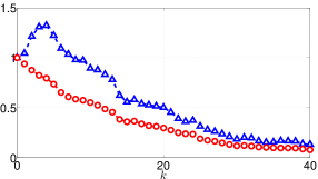
Figure 1: The sample means of the Lyapunov function (circle) and the Euclidean norm (triangle)

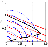
Figure 2: The averaged sample path (solid) and the level plots of the Lyapunov function (dashed) and the Euclidean norm (dotted)

Remark III.7

Since $\operatorname{supp}\mu$ is infinite in Example III.6, we cannot use the methods to construct a Lyapunov function for positive systems proposed in the literature (see, e.g., [8]).

IV Limiting Behavior of $p$th Mean Stability

This section studies the limiting behavior of $p$th mean stability as $p\to\infty$. We start with the following observation. Let $\mu$ be a probability distribution on $\mathbb{R}^{d\times d}$ and let $\mathcal{M}=\operatorname{supp}\mu$. Then the definitions of $p$-radius and joint spectral radius show $\rho_{p,\mu}\leq\hat{\rho}(\mathcal{M})$. Since $\rho_{p,\mu}$ is non-decreasing with respect to $p$ by Lemma II.4 we have

$$\lim_{p\to\infty}\rho_{p,\mu}\leq\hat{\rho}(\mathcal{M}).$$ (10)

It is then natural to ask when the equality holds in this inequality. We will show that the equality still holds under the following assumption, which is weaker than the one in [2].

Assumption IV.1

1. $\mathcal{M}$ leaves a proper cone invariant;

2. The singular part $\mu_{s}$ of $\mu$ consists of only point measures, i.e., $\mu_{s}=\sum_{i=1}^{N}p_{i}\delta_{M_{i}}$ for some positive numbers $p_{1},\dotsc,p_{N}$ and matrices $M_{1},\dotsc,M_{N}$.

The next theorem is the main result of this section.

Theorem IV.2

If $\mu$ satisfies Assumption IV.1 then

$$\lim_{p\to\infty}\rho_{p,\mu}=\hat{\rho}(\mathcal{M}).$$

This theorem has two corollaries, both of which can be proved easily using Proposition II.3. The first one shows a novel relationship between the stability of the deterministic switched system $\Sigma_{\mathcal{M}}$ and the stochastic switched system $\Sigma_{\mu}$.

Corollary IV.3

Assume that $\mu$ satisfies Assumption IV.1. Then $\Sigma_{\mathcal{M}}$ is absolutely asymptotically stable if and only if there exists $\gamma<1$ such that $\Sigma_{\mu}$ is $p$th mean stable with the decay rate at most $\gamma$; i.e., the expectation $E[\lVert x(k)\rVert^{p}]^{1/p}$ is of order $O(\gamma^{k})$ for every $p$.

The second corollary gives an expression of joint spectral radius.

Corollary IV.4

If $\mu$ satisfies Assumption IV.1 then

$$\hat{\rho}(\mathcal{M})=\lim_{p\to\infty}\rho\left(E[A^{\otimes p}]\right)^{1/p}.$$

To prove Theorem IV.2 we need the next lemma. Its proof is omitted due to limitations of space.

Lemma IV.5

Assume that $\mu$ satisfies Assumption IV.1. Then, for every $\epsilon>0$, there exists $\delta>0$ such that

$$\mu(\{X:X\geq^{K}(1-\epsilon)M\})\geq\delta$$

for every $M\in\mathcal{M}$.

Let us prove Theorem IV.2.

Proof of Theorem IV.2: By Proposition II.3 and the inequality (10) it is sufficient to show $\lim_{p\to\infty}\rho_{p,\mu}\geq\hat{\rho}(\mathcal{M})$. Let $\gamma:=\hat{\rho}(\mathcal{M})$. Let us take any cone linear absolute norm $\lVert\cdot\rVert$ with respect to the invariant cone. By Proposition II.5, we can show that there exist $C>0$ and $\{M_{k}\}_{k=1}^{\infty}\subset\mathcal{M}$ such that $\lVert M_{k}\dotsi M_{1}\rVert>C\gamma^{k}$ for infinitely many $k$.

Take arbitrary $\gamma_{1}$ and $\gamma_{2}$ such that $\gamma>\gamma_{1}>\gamma_{2}$. Define $\epsilon:=(\gamma-\gamma_{1})/\gamma$ and take the corresponding $\delta>0$ given by Lemma IV.5. Observe that, by Lemma I.2, if $X_{i}\geq^{K}(1-\epsilon)M_{i}=(\gamma_{1}/\gamma)M_{i}$ then $\lVert X_{k}\dotsi X_{1}\rVert\geq(\gamma_{1}/\gamma)^{k}\lVert M_{k}\dotsi M_{1}\rVert>C\gamma_{1}^{k}$. Therefore,

$$E[\lVert A_{k}\dotsi A_{1}\rVert^{p}]> \mu^{k}\left(\lVert A_{k}\dotsi A_{1}\rVert>C\gamma_{1}^{k}\right)\left(C\gamma_{1}^{k}\right)^{p}$$

$$\geq \left(\prod_{i=1}^{k}\mu(\{X_{i}:X_{i}\geq^{K}(1-\epsilon)M_{i}\})\right)C^{p}\gamma_{1}^{pk}$$

$$\geq \delta^{k}C^{p}\gamma_{1}^{pk}$$

and hence we have $E[\lVert A_{k}\dotsi A_{1}\rVert^{p}]^{1/kp}>C^{1/k}\delta^{1/p}\gamma_{1}$. Choose a sufficiently large $p_{0}$ such that $\delta^{1/p_{0}}\gamma_{1}>\gamma_{2}$. Then $E[\lVert A_{k}\dotsi A_{1}\rVert^{p_{0}}]^{1/kp_{0}}>C^{1/k}\gamma_{2}$ for infinitely many $k$. This implies $\rho_{p_{0},\mu}\geq\gamma_{2}$ and therefore $\lim_{p\to\infty}\rho_{p,\mu}\geq\gamma_{2}$. This completes the proof since $\gamma_{2}$ can be made arbitrary close to $\gamma=\hat{\rho}(\mathcal{M})$.

The next example gives a simple illustration of Theorem IV.2.

Example IV.6

Let $\mu$ be the uniform distribution on $[0,\gamma]$ for some $\gamma>0$. We can see that $\mu$ satisfies Assumption IV.1. Also clearly $\hat{\rho}(\mathcal{M})=\gamma$. On the other hand we have $\rho_{p,\mu}^{p}=\rho(E[A^{\otimes p}])=\gamma^{p}/(p+1)$. Therefore $\rho_{p,\mu}=\gamma(p+1)^{-p}$ and hence $\lim_{p\to\infty}\rho_{p,\mu}=\gamma=\hat{\rho}(\mathcal{M})$, as expected. We remark that, since $\operatorname{supp}\mu$ is infinite, we cannot apply the result in [2] to this example.

Finally the next theorem generalizes another characterization of joint spectral radius in [25], which does not need the existence of an invariant cone.

Theorem IV.7

If $\mu$ satisfies the condition b) of Assumption IV.1 then

$$\hat{\rho}(\mathcal{M})=\limsup_{p\to\infty}\left(\rho(E[A^{\otimes p}])\right)^{1/p}.$$ (11)

Sketch of the proof: Using Theorem IV.2 and the semidefinite lifting [2] of matrices one can show $\hat{\rho}(\mathcal{M})=\lim_{p\to\infty}\rho(E[X^{\otimes(2p)}])^{1/(2p)}$. Also it is possible to see that the sequence $\{\left(\rho(E[A^{\otimes p}])\right)^{1/p}\}_{p=1}^{\infty}$ is not decreasing. These observations yield (11).

V Markovian Case

So far we have restricted our attention to the case when the random variables $\{A_{k}\}_{k=0}^{\infty}$ are identically and independently distributed. In this section we study a more practical case of when the process $\{A_{k}\}_{k=0}^{\infty}$ is a time-homogeneous Markov chain. Let $\{\sigma_{k}\}_{k=0}^{\infty}$ be a time-homogeneous Markov chain taking values in $\{1,\dotsc,N\}$ with the transition probability matrix $\mathbb{P}=[p_{ij}]$ and the constant initial state $\sigma_{0}\in\{1,\dotsc,N\}$. Let $\mathcal{M}=\{M_{1},\dotsc,M_{N}\}$ be a set of $d\times d$ square matrices. We define the stochastic process $A=\{A_{k}\}_{k=0}^{\infty}$ by $A_{k}=M_{\sigma_{k}}$ and the switched system $\Sigma_{A}$ by

$$\Sigma_{A}:x(k+1)=A_{k}x(k).$$

The $p$th mean and moment stability of $\Sigma_{A}$ is defined in the same way as Definition II.1. Also we define the $L^{p}$-norm joint spectral radius $\rho_{p,A}$ of $A$ by (7).

The next theorem summarizes the relationship between $p$-radius, mean stability, and moment stability for the Markovian switched system $\Sigma_{A}$. Though the result actually holds for a general $p$, for simplicity of presentation we will restrict our attention to $p=1$ or $2$.

Theorem V.1

Assume that either $p=2$, or $\mathcal{M}$ leaves a proper cone $K$ invariant and $p=1$. Then the following conditions are equivalent.

1. $\rho_{p,A}<1$ for every $\sigma_{0}$;

2. $\Sigma_{A}$ is $p$th mean stable;

3. $\Sigma_{A}$ is $p$th moment stable;

4. Define the $Nd^{p}\times Nd^{p}$ matrix $T_{p}$ by

   $$T_{p}=(\mathbb{P}^{\top}\otimes I_{d^{p}})\operatorname{diag}(M_{1}^{\otimes p},\dotsc,M_{N}^{\otimes p}).$$

   Then $\rho(T_{p})<1$.

To prove this theorem we introduce the following definitions [5]. Let $x(\cdot;x_{0},\sigma_{0})$ denote the trajectory of $\Sigma_{A}$ with the initial conditions $x_{0}$ and $\sigma_{0}$. For each $k$ define $Q(k)=(Q_{i}(k),\dotsc,Q_{N}(k))\in(\mathbb{R}^{d})^{N}$ by $Q_{i}(k;x_{0},\sigma_{0}):=E[x(k;x_{0},\sigma_{0})_{\sigma_{k}=i}]$, and the operator $\mathcal{L}$ on $(\mathbb{R}^{d})^{N}$ by $\mathcal{L}(H):=(\mathcal{L}_{1}(H),\dotsc,\mathcal{L}_{N}(H))$ and $\mathcal{L}_{j}(H):=\sum^{n}_{i=1}p_{ij}A_{i}H_{i}$. The proof of the next lemma is omitted because it can be shown in the same way as [5].

Lemma V.2

Let $\mathcal{L}$ and $Q$ be as above.

1. $E[x(k;x_{0},\sigma_{0})]=\sum_{j=1}^{N}Q_{j}(k;x_{0},\sigma_{0})$.

2. $Q(k+1;x_{0},\sigma_{0})=\mathcal{L}(Q(k;x_{0},\sigma_{0}))$.

3. For every $H\in(\mathbb{R}^{d})^{N}$, $\operatorname{vec}{\mathcal{L}(H)}=T_{1}(\operatorname{vec}H)$.

With this lemma we can prove Theorem V.1.

Proof of Theorem V.1: The equivalence i) $\Leftrightarrow$ ii) $\Leftrightarrow$ iii) can be proved in the same way as Proposition II.3. Also, when $p=2$, the equivalence ii) $\Leftrightarrow$ iv) is proved in [5]. Therefore it is sufficient to show the implications iv) $\Rightarrow$ iii) and ii) $\Rightarrow$ iv) under the assumption that $p=1$ and $\mathcal{M}$ leaves a proper cone $K$ invariant

[iv) $\Rightarrow$ iii)]: Assume $\rho(T_{1})<1$ and let $x_{0}$ and $\sigma_{0}$ be arbitrary. Then, by Lemma V.2,

$$\operatorname{vec}Q(k;x_{0},\sigma_{0}) =\operatorname{vec}(\mathcal{L}^{k}(Q(0;x_{0},\sigma_{0})))$$

$$=T_{1}^{k}\operatorname{vec}Q(0;x_{0},\sigma_{0})\to 0,$$

which shows $Q(k;x_{0},\sigma_{0})\to 0$ as $k\to\infty$ and therefore $E[x(k;x_{0},\sigma_{0})]\to 0$ for all $x_{0}$ and $\sigma_{0}$. Thus $\Sigma_{A}$ is first moment stable.

[ii) $\Rightarrow$ iv)]: Omitted due to limitations of space.

The next corollary of Theorem V.1 enables us to compute $p$-radius efficiently.

Corollary V.3

If $p$ and $\mu$ satisfies the assumption in Theorem V.1 then it holds that

$$\rho_{p,A}=\rho(T_{p})^{1/p}.$$

Finally let us apply the results obtained in this section to the stabilization of Markovian switched systems Let

$$\begin{gathered}N=3,\ \mathbb{P}=\begin{bmatrix}0.3&0.5&0.2\\ 0.5&0.3&0.2\\ 0.2&0.2&0.6\end{bmatrix},\\ M_{1}=\begin{bmatrix}.32&.49\\ .24&.33\end{bmatrix},\ M_{2}=\begin{bmatrix}.53&.65\\ .75&.85\end{bmatrix},\ M_{3}=\begin{bmatrix}1.5&.51\\ .18&.69\end{bmatrix}.\end{gathered}$$

Corollary V.3 gives $\rho_{1,A}=1.221$ and therefore $\Sigma_{A}$ is not first mean stable. Let us consider the stabilization of $\Sigma_{A}$. Define the switched system with input by $x(k+1)=A_{k}x(k)+b_{k}u(k)$ where $b_{k}=n_{\sigma_{k}}$ with

$$n_{1}=\begin{bmatrix}-0.56\\ 0.39\end{bmatrix},\ n_{2}=\begin{bmatrix}0.40\\ -1.70\end{bmatrix},\ n_{3}=\begin{bmatrix}-0.37\\ -0.49\end{bmatrix}.$$

As an input we use the static state feedback $u(k)=fx(k)$ for some $f\in\mathbb{R}^{1\times 2}$. This yields the controlled system

$$\Sigma_{A+bf}:x(k+1)=(A_{k}+b_{k}f)x(k)$$

Let $f=\begin{bmatrix}0.36&0.50\end{bmatrix}$. Then all the matrices $M_{i}+n_{i}f$ ($i=1,2,3$) have only positive entries. Therefore we can use Corollary V.3 to find $\rho_{1,A+bf}=0.9554$. Therefore the controlled system $\Sigma_{A+bf}$ is first mean stable by Theorem V.1. Fig. 3

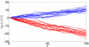
Figure 3: Sample paths of switched systems. Dashed: Before stabilization. Solid: After stabilization

shows the 20 sample paths of the original switched system and the stabilized switched system. Finding a systematic way to obtain a stabilizing feedback gain is left as an open problem.

VI Conclusion

We investigated the mean stability of a class of discrete-time stochastic switched systems. First we presented the equivalence between mean stability and the existence of a homogeneous Lyapunov function. Then we showed that, in the limit of $p\to\infty$, the $p$th mean stability becomes equivalent to the absolute asymptotic stability of an associated deterministic switched system. Finally the characterization of the stability of a class of Markovian switched systems was given. Throughout the paper $L^{p}$-norm joint spectral radius has played a key role.

References

- [1] A. Berman and R. J. Plemmons, Nonnegative Matrices in the Mathematical Sciences. Philadelphia: SIAM, 1979.
- [2] V. D. Blondel and Y. Nesterov, “Computationally efficient approximations of the joint spectral radius,” SIAM Journal on Matrix Analysis and Applications, vol. 27, no. 1, pp. 256–272, 2005.
- [3] V. I. Bogachev, Measure Theory. Berlin, Heidelberg: Springer Berlin Heidelberg, 2007.
- [4] J. Brewer, “Kronecker products and matrix calculus in system theory,” IEEE Transactions on Circuits and Systems, vol. 25, no. 9, pp. 772–781, 1978.
- [5] O. Costa and M. Fragoso, “Comments on “Stochastic stability of jump linear systems”,” IEEE Transactions on Automatic Control, vol. 49, no. 8, pp. 1414–1416, 2004.
- [6] X. Dai, Y. Huang, and M. Xiao, “Almost sure stability of discrete-time switched linear systems: a topological point of view,” SIAM Journal on Control and Optimization, vol. 47, no. 4, pp. 2137–2156, 2008.
- [7] W. Dayawansa and C. Martin, “A converse Lyapunov theorem for a class of dynamical systems which undergo switching,” IEEE Transactions on Automatic Control, vol. 44, no. 4, pp. 751–760, 1999.
- [8] T. S. Doan, A. Kalauch, and S. Siegmund, “A constructive approach to linear Lyapunov functions for positive switched systems using Collatz-Wielandt sets,” IEEE Transactions on Automatic Control, vol. 58, no. 3, pp. 748–751, 2013.
- [9] Y. Fang and K. A. Loparo, “On the relationship between the sample path and moment Lyapunov exponents for jump linear systems,” IEEE Transactions on Automatic Control, vol. 47, no. 9, pp. 1556–1560, 2002.
- [10] ——, “Stochastic stability of jump linear systems,” IEEE Transactions on Automatic Control, vol. 47, no. 7, pp. 1204–1208, 2002.
- [11] Y. Fang, K. A. Loparo, and X. Feng, “Almost sure and -moment stability of jump linear systems,” International Journal of Control, vol. 59, no. 5, pp. 1281–1307, 1994.
- [12] M. D. Fragoso and O. L. V. Costa, “A unified approach for stochastic and mean square stability of continuous-time linear systems with Markovian jumping parameters and additive disturbances,” SIAM Journal on Control and Optimization, vol. 44, no. 4, pp. 1165–1191, 2005.
- [13] R. M. Jungers, The Joint Spectral Radius, ser. Lecture Notes in Control and Information Sciences. Berlin, Heidelberg: Springer Berlin Heidelberg, 2009, vol. 385.
- [14] R. M. Jungers and V. Y. Protasov, “Weak stability of switching dynamical systems and fast computation of the -radius of matrices,” in 49th IEEE Conference on Decision and Control, 2010, pp. 7328–7333.
- [15] ——, “Fast methods for computing the -radius of matrices,” SIAM Journal on Scientific Computing, vol. 33, no. 3, pp. 1246–1266, 2011.
- [16] F. Kozin, “A survey of stability of stochastic systems,” Automatica, vol. 5, no. 1, pp. 95–112, 1969.
- [17] A. Molchanov and Y. Pyatnitskiy, “Criteria of asymptotic stability of differential and difference inclusions encountered in control theory,” Systems & Control Letters, vol. 13, pp. 59–64, 1989.
- [18] M. Ogura and C. Martin, “Generalized joint spectral radius and stability of switching systems,” Linear Algebra and its Applications, vol. 439, no. 8, pp. 2222–2239, 2013.
- [19] V. Y. Protasov, “The generalized joint spectral radius. A geometric approach,” Izvestiya: Mathematics, vol. 61, no. 5, pp. 995–1030, 1997.
- [20] T. I. Seidman, H. Schneider, and M. Arav, “Comparison theorems using general cones for norms of iteration matrices,” Linear Algebra and its Applications, vol. 399, pp. 169–186, 2005.
- [21] J. Theys, “Joint Spectral Radius: theory and approximations,” Ph.D. dissertation, Universit’e Catholique de Louvain, 2005.
- [22] J. N. Tsitsiklis and V. D. Blondel, “The Lyapunov exponent and joint spectral radius of pairs of matrices are hard – when not impossible – to compute and to approximate,” Mathematics of Control, Signals, and Systems, vol. 10, no. 1, pp. 31–40, 1997.
- [23] J. S. Vandergraft, “Spectral properties of matrices which have invariant cones,” SIAM Journal on Applied Mathematics, vol. 16, no. 6, pp. 1208–1222, 1968.
- [24] A. N. Vargas and J. B. R. do Val, “Average cost and stability of time-varying linear systems,” IEEE Transactions on Automatic Control, vol. 55, no. 3, pp. 714–720, 2010.
- [25] J. Xu and M. Xiao, “A characterization of the generalized spectral radius with Kronecker powers,” Automatica, vol. 47, no. 7, pp. 1530–1533, 2011.