Dynamics of the envelope of a rapidly rotating star or giant planet in gravitational contraction

Abstract

Aims. We wish to understand the processes that control the fluid flows of a gravitationnally contracting and rotating star or giant planet.

Methods. We consider a spherical shell containing an incompressible fluid that is slowly absorbed by the core so as to mimick gravitational contraction. We also consider the effects of a stable stratification that may also modify the dynamics of a pre-main sequence star of intermediate mass.

Results. This simple model reveals the importance of both the Stewartson layer attached to the core and the boundary conditions met by the fluid at the surface of the object. In the case of a pre-main sequence star of intermediate mass where the envelope is stably stratified, shortly after the birth line, the spin-up flow driven by contraction overwhelms the baroclinic flow that would take place otherwise. This model also shows that for a contracting envelope, a self-similar flow of growing amplitude controls the dynamics. It suggests that initial conditions on the birth line are most probably forgotten. Finally, the model shows that the shear (Stewartson) layer that lies on the tangent cylinder of the core is likely a key feature of the dynamics that is missing in 1D models. This layer can explain the core and envelope rotational coupling that is required to explain the slow rotation of cores in giant and subgiant stars.

1 Introduction

The influence of rotation has long been known to be crucial for understanding mixing in radiative regions of stars and interpreting the observed surface abundances Strittmatter (1969). Many (if not all) stellar evolution codes now include some modelling of the transport of angular momentum and chemical elements by the flows induced by rotation in the stably stratified radiative zones. The difficulty is that stellar evolution code are one-dimensional while fluid flows are generally multi-dimensional. Basically, two types of modelling are currently used: one is based on a simple (turbulent) diffusion process (e.g. Pinsonneault, 1997) and the other includes a first-order modelling of meridional advection, distinguishing the transport of angular momentum and that of chemicals Zahn (1992). However, both of them need adjustment of diffusion coefficients with respect to observations. While this modelling has succeeded in explaining various features of abundances pattern or evolutionary effects like the surface abundance of lithium as a function of mass Charbonnel & Talon (1999), the (relative) high number of red super-giants in low-metallicity galaxies Maeder & Meynet (2001), or the ratio of type Ibc to type II supernovae Meynet & Maeder (2005), many recent results challenge our understanding of this so-called rotational mixing. One of the most famous is the distribution of LMC B-stars in a diagram plotting the nitrogen abundance versus the rotational velocity (the so-called Hunter diagram). As shown by Brott et al. (2011), many slowly rotating stars show overabondance of nitrogen compared to the predictions of models while some fast rotating stars show much less nitrogen than expected.

In order to progress in this difficult problem, it is clear that a better view of the dynamics of rotating stars is needed. Many processes contribute to rotational mixing. Let us recall that the time scale of element transport inside stars is essentially controlled by the radiative zones. Indeed, convective regions mix almost instantaneously. When the star is non-rotating elements may migrate through radiative regions thanks to microscopic diffusive processes or propagating waves. In rotating stars radiative regions are no longer at rest: beyond the global rotation baroclinic flows arise as a differential rotation and an associated meridional circulation Rieutord (2006b). While meridional currents can obviously carry elements from deep to surface layers, differential rotation can also contribute to the transport through shear driven instabilities and associated turbulence. As pointed out by Zahn (1992), baroclinicity may be helped by angular momentum losses resulting from mass loss. To be complete, a sequence of gravitational contraction may also drive a redistribution of angular momentum and elements during the pre-main sequence or just at the end of the main sequence.

Going beyond the above mentioned modelling of rotational mixing requires relaxing the spherical symmetry of the models. A first step in this direction is to simplifies the structure of the stars so as to focus on its interior hydrodynamics. This line of research was followed in Rieutord (2006a). The star was reduced to a spherical ball filled with an incompressible fluid in order to study the properties of the baroclinic flows. Besides giving a simplified view of the dynamic processes controlling a radiative zone, this work lead to a simplified set-up for boundary conditions in complete (compressible) two-dimensional models of fast rotating stars Espinosa Lara & Rieutord (2013). In the present paper we address the effect of mass-contraction/expansion of a star or a giant planet on the global flows that affect the envelope of the rotating object. Although this driving results from the compressibility of the fluid, we decided to investigate its consequences using an incompressible fluid. The contraction/expansion of the envelope is mimicked by a core that absorbs or injects matter at a constant rate in a surrounding stably or neutrally stratified envelope. We wish to determine the resulting flows and the circumstances when it overwhelms the eventual baroclinic flows. This will complete the work of Rieutord & Beth (2014) who studied this same competition in the case of a spin-down driven by mass-losses.

The paper is organized as follows : In section 2 we describe the model and the questions of fluid dynamics that are addressed. We next consider the case where outer boundary conditions are no-slip and use the ensuing analytical solutions to enlight the dynamics (section 3). In section 4, we discuss the presumably more realistic case with stress-free boundary conditions. Conclusions and discussion of extrapolations of the results to models with a compressible fluid follow.

2 The model

2.1 Description

For modelling in a simple way the contracting/expanding star or giant planet, we consider a self-gravitating incompressible viscous fluid enclosed between two spherical shells. These shells are assumed not to be distorted by rotation. The inner shell may represents a core-envelope boundary through which a flux of matter is imposed. This flux is described by a uniform radial velocity $V_{s}$ at this interface. For a contracting envelope, $V_{s}$ is negative. Note that as the fluid of the envelope enters the core and as its radius is assumed fixed, the core’s density linearly increases with time, namely

$$\rho_{\rm core}=\rho_{0}\left(1+\frac{t}{t_{s}}\right)$$

where we introduced the initial density of the core $\rho_{0}$ and the “suction time”, the time the core needs to increase its density by a factor $2$, namely

$$t_{s}=\frac{R_{\rm core}}{3V_{s}}\tilde{\rho}$$ (1)

where $\tilde{\rho}=\frac{\rho_{0}}{\rho}$. This time is of same order of magnitude as the Kelvin-Helmholtz time. Here, $\rho$ is the density of the envelope. We note that changing the sign of $V_{s}$ can readily describe an expanding envelope due to a wind. The outer bounding sphere is of constant radius and lets matter going through so as to insure mass conservation in the envelope.

2.2 A digest of the following Fluid Dynamics

The following of the paper is basically fluid dynamics. We thought that the reader interested in the astrophysical implications of the results might also be interested in a summary of the various steps that are described below. The reader may then jump to the discussion at the end of the paper.

As it is well known, the contraction of the star together with the conservation of angular momentum induces a global acceleration of the rotation rate, namely a spin-up, of the star. The problem of spin-up flows has been considered many times in the fluid dynamics literature (see the review of Duck & Foster, 2001). However, these studies have been mostly motivated by engineering applications and therefore have considered a driving by boundaries and not, as in our case, by a radial flow. The influence of a stable stratification, that we need to know in order to deal with radiative regions of stars, has been more seldom considered in astrophysically relevant geometries. The most relevant study is certainly the work of Friedlander (1976) who considered the spin-down of the radiative core of the Sun through Reynolds stresses at the interface of the convective and radiative regions. So, here too, the driving of the flows is by the boundaries. Friedlander’s model is much simplified (as ours) as it uses the Boussinesq approximation (i.e. neglecting the compressibility of the fluid). It also neglects baroclinic flows associated with this set-up. This work however establishes that the spin-down (or spin-up) time scale of a stably stratified fluid is the classical Eddington-Sweet time scale, namely the product of the heat diffusion time scale (also known as Kelvin-Helmholtz time scale) and the factor $({\cal N}/2\Omega)^{2}$, where ${\cal N}$ is the Brunt-Väisälä frequency in the radiative region and $\Omega$ is the rotation rate. In slowly rotating stars the Eddington-Sweet time scale is much longer than the Kelvin-Helmholtz, but in fast rotators that are considered here, these time scales are similar. Hence, the spin-up driven by a gravitational contraction has never been considered in the literature as far as we know.

The first step of our analysis considers the case of a neutrally stratified envelope like the one met in a star with an outer convection zone. The translation of this constant entropy medium into the incompressible fluid model is the simple constant density fluid. This simple model allows us to derive an asymptotic solution for small Ekman numbers (i.e. small viscosity as appropriate for stellar applications). This solution shows that the spinning up core controls the flow inside its tangent cylinder and gives the amplitude of the quasi-steady flow there. Outside the tangent cylinder we find that the solution depends very much on the outer boundary conditions. We analyse the rather artificial case where no-slip conditions are imposed on the outer boundary, since this case also allows the derivation of an analytic asymptotic solution. Moreover, with these boundary conditions, we can also solve the case where the envelope is stably stratified (but not contracting) and derive the associated differential rotation forced by the baroclinic torque.

The competition between the two forcings (spin-up and baroclinicity) necessarily arises in the pre-main sequence phase of an intermediate mass star. We indeed expect that for such a mass range, an outer radiative envelope sets in after the birth line, likely after the disappearance of convective flows (e.g. Maeder, 2009).

With our simplified model we can appreciate the result of this competition. As a first step, still using the artificial no-slip outer boundary condition, we compare the amplitudes of the baroclinic flow and the contraction-driven spin-up flow when they are taken separately. It gives us a criterion on the parameters of the star. Using numerical solutions of the full problem (including simultaneously the two forcing mechanisms), we confirm the validity of the criterion.

Our next step is to leave aside the no-slip outer boundary condition and concentrate on the more realistic stress-free condition. In such a case, the derivation of an asymptotic analytic solution is much more involved and we had to resort to numerics. Numerical solutions show that outside the tangent cylinder of the core, a steady spin-up flow of an unstratified fluid driven by contraction has an amplitude that scales with the ratio of two small parameters, namely Ro/E, where Ro is the Rossby number measuring the driving and E is the Ekman number measuring the viscosity. With stellar parameters this ratio is expected to be larger than unity showing that a steady solution is necessarily of high amplitude. In addition, the time needed to reach such a steady state is of the order of the contraction time, thus suggesting that this steady state is actually never reached. This result prompted us to study the transient state of the spin-up flow first without stratification and then accounting for a stable stratification in the envelope. Before the transient state reaches a significant amplitude, it can be studied with linear equations that are easier to solve. Remarkably enough, this transient flow shows the emergence of a quasi-self-similar solution that simply grows in amplitude in the volume outside the core’s tangent cylinder. Since our original question is to know whether such flow is able to supersede the baroclinic flow driven by the combination of rotation and stratification, we compared the two flows. The easy way is to compare the amplitudes of the flow taken separately and quite clearly we find that the contraction-induced spin-up rapidly overtakes the amplitude of a baroclinic flow. The numerical solution of the transient starting from an established baroclinic flow confirms this result.

We now present the detailed derivation of these fluid dynamics results, but the hurried reader more interested in the astrophysical side of the problem may now jump to the discussion in section 5.

2.3 Equations of motion

In an inertial frame, the dynamics of an incompressible fluid enclosed within the two shells is governed by the equations of momentum and mass conservation :

$$\left\{\begin{array}[]{ccl}\frac{\partial\@vec{v}}{\partial t}+(\@vec{v}\cdot\@vec{\nabla})\@vec{v}=-\frac{1}{\rho}\@vec{\nabla}P+\nu\Delta\@vec{v}\\ \@vec{\nabla}\cdot\@vec{v}=0\end{array}\right.$$ (2)

where $\@vec{v}$ is the velocity field, $P$ the pressure and $\nu$ the kinematic viscosity of the envelope. Let us now remove the bulk rotation and set

$$\@vec{v}=\@vec{\Omega}\wedge\@vec{r}+\@vec{w}\;.$$ (3)

We define $\@vec{\Omega}$ as the angular velocity of the core. Since the field $\@vec{v}$ is axisymmetric,

$$(\@vec{v}\cdot\@vec{\nabla})\@vec{v}=\@vec{\Omega}\wedge(\@vec{\Omega}\wedge\@vec{r})+2\@vec{\Omega}\wedge\@vec{w}+(\@vec{w}\cdot\@vec{\nabla})\@vec{w}\;.$$

where we recognise the centrifugal and Coriolis accelerations. The centrifugal potential is gathered with the pressure into $\Pi$. Substituting (3) in the set of equations (2), we find that the relative velocity $\@vec{w}$ verifies

$$\left\{\begin{array}[]{ccl}\frac{\partial\@vec{w}}{\partial t}+2\@vec{\Omega}\wedge\@vec{w}+(\@vec{w}\cdot\@vec{\nabla})\@vec{w}=-\@vec{\nabla}\Pi+\nu\Delta\@vec{w}-\@vec{\dot{\Omega}}\wedge\@vec{r}\\ \@vec{\nabla}\cdot\@vec{w}=0\end{array}\right.$$ (4)

Let us note that the RHS-term now depends on the acceleration of the rotation rate of the core $-\@vec{\dot{\Omega}}\wedge\@vec{r}$ where $\@vec{\dot{\Omega}}$ needs to be determined.

2.4 Scaled equations and linearization

We scale the equations using the Kelvin-Helmholtz time scale $\frac{R}{V_{s}}$, which is the time scale of the complete absorption of the envelope by the core. The length scale $R$ is the outer radius of the envelope, and the velocity scale is the suction velocity $\@vec{w}=V_{s}\@vec{u}$. The system (4) now reads

$$\left\{\begin{array}[]{ccl}Ro\frac{D\@vec{u}}{D\tau}+\@vec{e}_{z}\wedge\@vec{u}=-\@vec{\nabla}p+E\Delta\@vec{u}-\dot{\omega}\@vec{e}_{z}\wedge\@vec{r}\\ \@vec{\nabla}\cdot\@vec{u}=0\end{array}\right.$$ (5)

where $p$ is the reduced pressure. The following dimensionless numbers appear :

$$\dot{\omega}=\frac{\dot{\Omega}R}{2\Omega V_{s}},\quad Ro=\frac{V_{s}}{2\Omega R},\quad E=\frac{\nu}{2\Omega R^{2}}$$ (6)

Here we introduced the non-dimensional acceleration of the core rotation rate $\dot{\omega}$, a Rossby number $Ro$ and the Ekman number $E$ which measures the viscosity of the envelope.

Obviously, the suction velocity is very small compared to the rotation one. Hence, we expect $Ro\ll 1$. As a first step setting $Ro=0$ seems reasonable as long as $Ro\,u$ is less than unity (so as to be able to neglect quadratic terms). Thus doing, we are left with a steady state problem which describes the quasi-steady evolution of the system as long as the non-dimensional time $\tau$ verifies:

$$Ro\ll\tau\ll\tau_{s}$$ (7)

where $\tau_{s}=\frac{\eta\tilde{\rho}}{3}$ is the scaled suction time ($\eta=\frac{R_{core}}{R}$ is the scaled inner radius). $\tau\gg Ro$ means that we neglect the transients corresponding to a few rotation periods where boundary layers form. Likewise, $\tau\ll\tau_{s}$ means that the rotation rate has not been changed, namely that $\dot{\Omega}t\ll\Omega$.

2.5 The acceleration of the core

2.5.1 General equation

Equations (5) need the expression of $\dot{\omega}$. By absorbing the envelope, the mass of the core grows, as its angular momentum. Evolution of the angular momentum $L_{z}$ of the core is governed by

$$\frac{d{L_{z}}}{dt}=\@vec{e}_{z}\cdot\{-\int_{(S)}(\@vec{r}\wedge\rho\@vec{v})\@vec{v}\cdot\@vec{dS}+\int_{(S)}\@vec{r}\wedge[\sigma]\@vec{dS}\}$$ (8)

The first integral is the flux of incoming angular momentum and the second one is the viscous torque applied on the core surface. $[\sigma]$ is the stress tensor. We have

$$\@vec{e}_{z}\cdot(\@vec{r}\wedge[\sigma]\@vec{e_{r}})=r\sin\theta\sigma_{r\phi}=r\sin\theta\rho\nu\left.\frac{\partial w_{\phi}}{\partial r}\right|_{r=R_{core}}$$ (9)

Besides, for a sphere of mass $M_{core}$ and radius $\eta R$ :

$$\@vec{L}=I\@vec{\Omega}=\frac{2}{5}M_{core}(\eta R)^{2}\@vec{\Omega}$$ (10)

With the previous scaling, we get

$$\begin{array}[]{ccl}M_{core}\dot{\Omega}&=&\frac{8\pi}{3}\Omega\rho V_{s}(\eta R)^{2}\\ &+&5\pi\nu\rho V_{s}\eta\displaystyle\int_{0}^{\pi}\sin^{2}\theta\left.\frac{\partial u_{\phi}}{\partial r}\right|_{r=\eta}d\theta\\ \end{array}$$ (11)

The evaluation of the remaining integral needs the expression of the azimuthal flow $u_{\phi}$ at the core-envelope boundary $r=\eta$, namely in the Ekman boundary layers.

2.5.2 Boundary layer analysis

First of all, we change the boundary conditions with mass-flux to ordinary boundary condition by making the substitution

$$\@vec{u}=\@vec{u^{\prime}}-\frac{\eta^{2}}{r^{2}}\@vec{e}_{r}$$

The new velocity field $\@vec{u^{\prime}}$ verifies

$$\left\{\begin{array}[]{ccl}\@vec{\nabla}\wedge\{\@vec{e}_{z}\wedge\@vec{u^{\prime}}-E\Delta\@vec{u^{\prime}}\}&=&2(\frac{\eta^{2}}{r^{3}}-\dot{\omega})\cos\theta\@vec{e}_{r}\\ &+&(\frac{\eta^{2}}{r^{3}}+2\dot{\omega})\sin\theta\@vec{e}_{\theta}\\ \@vec{\nabla}\cdot\@vec{u^{\prime}}&=&0\end{array}\right.$$ (12)

with the boundary conditions

$$\@vec{u}^{\prime}=\@vec{0}\qquad{\rm on}\qquad r=\eta$$

and

$$\@vec{e}_{r}\times[\sigma]\@vec{e}_{r}=\@vec{0},\qquad{\rm and}\qquad u^{\prime}_{r}=0\qquad{\rm on}\qquad r=1$$

These latter conditions describe stress-free boundary conditions. Indeed, we assume that the upper layers outside the outer shell have unimportant dynamic effects and are just providing/absorbing some mass. In the following, we drop the prime on the velocity field.

As shown in Espinosa Lara & Rieutord (2013), the Ekman number in stars is always very small thus leading to the formation of boundary layers near the boundaries. To derive the expression of the flow, we therefore examine the asymptotic case $E\ll 1$. We first note that if we consider the inviscid case $E=0$, the set of equations (12) is solved by

$$\left\{\begin{array}[]{ccl}\bar{u}_{r}&=&\frac{\eta^{2}}{r^{2}}+r\dot{\omega}\left(2-3\sin^{2}\theta\right)\\ \bar{u}_{\theta}&=&-3r\dot{\omega}\sin\theta\cos\theta\\ \end{array}\right.$$ (13)

In the azimuthal direction, we look for a flow such as $\bar{u}_{\phi}=U(s)\@vec{e_{\phi}}$ as dictated by the Taylor-Proudman theorem (e.g. Greenspan, 1969). Such a flow does not verify the no-slip boundary conditions at the interface $r=\eta$. It needs boundary layer corrections so as to satisfy $\bar{u}_{0}+\widetilde{u}_{0}=0$. The bar refers to the solution within the envelope i.e. outside the boundary layer and tilded quantities are for boundary layer corrections.

Following Rieutord (2006a) we write the boundary layer corrections as:

$$(\@vec{n}\wedge\widetilde{u}_{0}+i\widetilde{u}_{0})=-(\@vec{n}\wedge\bar{u}_{0}+i\bar{u}_{0})_{\alpha=0}\exp{(-(1-i)\alpha)}$$ (14)

where $\displaystyle{\alpha=(r-\eta)\sqrt{\frac{|\cos\theta|}{2E}}}$ and $\@vec{n}=-\@vec{e}_{r}$. We only keep the decreasing solution. The corrections thus read

$$\left\{\begin{array}[]{ccl}\widetilde{u}_{\theta}&=&\displaystyle{-U(\eta\sin\theta)\ \sin\alpha\ e^{-\alpha}}\\ \widetilde{u}_{\phi}&=&\displaystyle{-U(\eta\sin\theta)\ \cos\alpha\ e^{-\alpha}}\end{array}\right.$$ (15)

As in Rieutord (2006a), mass conservation gives the relation between the Ekman pumping $\widetilde{u}_{r}$ and the geostrophic flow $U$. It yields

$$1+(2-3\sin^{2}\theta)\eta\dot{\omega}=\frac{1}{\eta\sin\theta}\sqrt{\frac{E}{2}}\frac{\partial}{\partial\theta}\left(\frac{\sin\theta\ U(\eta\sin\theta)}{\sqrt{|\cos\theta|}}\right)$$ (16)

where we keep only $\mathcal{O}(\sqrt{E})$ terms. Integrating with respect to $\theta$, we get

$$U(\eta\sin\theta)=\eta\sqrt{\frac{2}{E}}\frac{{\sqrt{|\cos\theta|}}}{\sin\theta}\left(1-\cos\theta+\eta\dot{\omega}\cos\theta\sin^{2}\theta\right)$$ (17)

Note that this expression defines $U$ only within the tangent cylinder of the core defined as $s=r\sin\theta=\eta$ ($s$ is the radial cylindrical coordinate).

Near the surface $r=\eta$ i.e. within the boundary layer, the shear is dominated by the boundary layer correction. It simplifies the computation of the radial derivative of the azimuthal flow $u_{\phi}$ which reads

$$\frac{\partial u_{\phi}}{\partial r}=\frac{\eta}{E}|\cot\theta|\left(1-\cos\theta+\eta\dot{\omega}\cos\theta\sin^{2}\theta\right)$$ (18)

Integral in (LABEL:eq6) can now be evaluated:

$$\int_{0}^{\pi}\sin^{2}\theta\left.\frac{\partial u_{\phi}}{\partial r}\right|_{r=\eta}d\theta=\eta\frac{2}{3E}\left(\frac{1}{2}+\frac{2}{5}\eta\dot{\omega}\right)$$ (19)

We can now derive the acceleration of the angular velocity of the core. Considering quasi-steady solutions that arise when $Ro\ll\tau\ll\tau_{s}$, (LABEL:eq6) leads to

$$\dot{\omega}=\frac{9}{4\tilde{\rho}\eta}$$ (20)

which completes the equations (12).

The foregoing solution (17) shows that the differential rotation driven by the mass contraction scales as $\mathcal{O}(E^{-1/2})$. It means that the linear regime that we solved is valid only when $Ro\ll\sqrt{E}$, which is actually the case (see below). The foregoing solution however describes the fluid flow only within the tangent cylinder of the core.

Outside the cylinder, the solution depends on the outer boundary conditions and on the Stewartson layer that lies upon the cylinder. This makes the global solution quite involved, all the more that we should also account for a possible stable stratification of the envelope. Indeed, during the PMS phase of intermediate mass stars, the envelope is completely radiative. Therefore the contraction-induced differential rotation competes with the one induced by the baroclinicity of the envelope.

Before getting any further, we need evaluating stellar numbers that have appeared.

2.6 Orders of magnitude

As a test case of the foregoing problem, we first consider the contraction of a fully radiative 3 M_⊙ PMS star. On the birthline, its surface temperature is around $T_{*}\sim 5600K$, its luminosity $L_{*}\sim 10^{2}L_{\odot}$ and its radius is $R_{*}\sim 10^{10}\text{m}$. The young star contracts on the Kelvin-Helmholtz time upon the PMS (Henyey) track, namely:

$$t_{\rm KH}=\frac{GM^{2}}{RL}$$

according to Maeder (2009). This leads to $t_{\rm KH}\sim 2.6\leavevmode\nobreak\ 10^{5}\text{yr}$.

Setting arbitrarily $R_{\rm core}=0.15R_{*}$, we find $V_{s}\sim 6\times 10^{-5}\text{m.s${}^{-1}$}$. Considering a rotation velocity of 10 km/s (such that near the end of the PMS after a gravitational contraction at constant angular momentum we obtain a star like HD 37806 studied by Boehm & Catala 1995) we find a Rossby number

$$Ro\sim 3\times 10^{-9}$$

which is very small as expected.

The estimate of the Ekman number requires a value of the kinematic viscosity. If we use Zahn’s prescription Zahn (1992) for a turbulent viscosity, we get $\nu\sim 10^{4}\text{ m${}^{2}\cdot$s${}^{-1}$}$ and thus

$$E\sim 10^{-10}$$

With the radiative viscosity (e.g. Espinosa Lara & Rieutord, 2013), $\nu\sim 10^{2}\text{ m${}^{2}\cdot$s${}^{-1}$}$, we get

$$E\sim 10^{-12}$$

For both values the condition $Ro\ll\sqrt{E}$ is satisfied.

During the contraction, the quasi-steady state within the cylinder is reached after a spin-up time, namely after $\frac{(2\Omega)^{-1}}{\sqrt{E}}$. Using the previous numbers, we find that this state occurs after $\sim 10^{3}$ or $10^{4}$ years so rather shortly after the start of contraction. Therefore, within the tangent cylinder, we can neglect the transient phase.

If we consider the contracting envelope of a Jupiter-like giant planet, Ekman numbers are also very small although with larger uncertainties: Ogilvie & Lin (2004) give $E\sim 10^{-7}$ while Wu (2005) suggest $E\sim 10^{-13}$. The typical contraction time of giant planets is over 1 Gyrs Fortney & Nettelmann (2010) so that $Ro\sim P_{\rm rot}/t_{\rm contraction}\sim 10^{-12}$. The condition $Ro\ll\sqrt{E}$ is also easily satisfied.

2.7 Adding stratification

2.7.1 Scaled equations

To account for a stable stratification in the envelope we now generalize the set of equations (12) by taking into account the buoyancy force and the equation for temperature fluctuations. In PMS stars the stable stratification of the envelope may come after a convective episode and thus may be evolving with time. To simplify and get an upper bound on the effects of stratification we take the Brunt-Väisälä frequency as constant in time.

To be consistent with the foregoing model that uses an incompressible fluid we use the Boussinesq approximation. Following Rieutord (2006a) and combining with (12) we find

$$\left\{\begin{array}[]{l}\@vec{\nabla}\times(\@vec{e}_{z}\wedge\@vec{u}-B\theta_{T}\@vec{r}-E\Delta\@vec{u})=-Bn_{T}^{2}\sin{\theta}\cos{\theta}\@vec{e}_{\phi}\\ -2(\frac{\eta^{2}}{r^{3}}+\dot{\omega})\cos\theta\@vec{e}_{r}+(\frac{\eta^{2}}{r^{3}}+2\dot{\omega})\sin\theta\@vec{e}_{\theta}\\ \\ (n_{T}^{2}/r)u_{r}=B\tilde{E}_{T}\Delta\theta_{T}\\ \\ \@vec{\nabla}\cdot\@vec{u}=0\end{array}\right.$$ (21)

We use the same scales and notations as Rieutord (2006a). The temperature perturbation is scaled as $\delta T=\epsilon T_{*}\theta_{T}$ where $\epsilon=\frac{\Omega^{2}R}{g_{s}}$ is the ratio of centrifugal acceleration to surface gravity. Recall that the centrifugal acceleration is driving the baroclinic flow. The Brunt-Väisälä profile $n_{T}^{2}$ is scaled with $\mathcal{N}^{2}=\frac{\alpha T_{*}g_{S}}{R}$ where $\alpha$ is the dilation coefficient and $g_{s}$ the surface gravity.

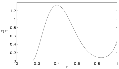
Figure 1: The typical and scaled Brunt-Väisälä frequency profile as a function of the normalized radius with $\eta=0.15$.

The dimensionless number $B$ monitors the ratio of the forcings. From the expression of the scaling of the baroclinic flow (see Rieutord, 2006a), we have

$$B=\frac{\epsilon\mathcal{N}^{2}R}{2\Omega V_{s}}$$ (22)

Finally, the dimensionless number

$$\tilde{E}_{T}=\frac{E}{\lambda}\qquad{\rm with}\quad\lambda=\mbox{${\cal P}$}\frac{{\cal N}^{2}}{4\Omega^{2}}$$ (23)

measures heat diffusion. ${\cal P}$ is the Prandtl number. For fast rotators, $\lambda$ is a small parameter which we set to $10^{-4}$ following the estimate of Rieutord & Beth (2014).

Based on stellar models, a typical profile of the Brunt-Väisälä frequency is shown in Fig. 1. We use the polynomial expression

$$\left\{\begin{array}[]{ccl}n_{T}^{2}(r)&=&0\text{ if }r<\eta\\ \\ n_{T}^{2}(r)&=&(\alpha(r-\eta)+\beta(r-\eta)^{2}+\gamma(r-\eta)^{3})^{2}\text{ if }r\in[\eta;1].\end{array}\right.$$ (24)

to represent this function. $\alpha$, $\beta$ and $\gamma$ are the coefficients resulting from the polynomial fit.

3 An interesting solution with rigid outer boundary conditions

Before getting into the full numerics, it is interesting to consider the case where the outer bounding sphere of the envelope is rigidly rotating at the same rate as the inner core. Outer no-slip conditions can be expected if a turbulent layer threaded by magnetic fields covers the stellar surface (see Rieutord & Beth, 2014), however the synchronism between this layer and the surface is here an ad hoc assumption (which can be easily removed actually). The interesting point that is addressed below comes from the simple analytical solutions that can be derived for the flow outside the tangent cylinder and which gives an interesting view of the properties of the system.

3.1 The steady mass contraction induced flow

With no-slip conditions on the outer boundary $r=1$, we may easily derive the expression of the geostrophic flow out of the tangent cylinder of the core. When no stratification is present, the azimuthal velocity reads

$$U(s)=\sqrt{\frac{2}{E}}(1-s^{2})^{3/4}\left(\frac{\eta^{2}}{s}-\dot{\omega}s\right)\qquad s\geq\eta$$ (25)

As shown in Fig. 2, this analytical solution nicely matches the numerical one.

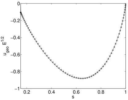
Figure 2: Comparison between numerical (solid line) and analytical (star line) solutions of the geostrophic flow at the equator $u_{\phi}(r,\theta=\frac{\pi}{2})$ for $E=10^{-7}$, $\eta=0.15$, $\tilde{\rho}=10$ without stratification when the envelope is rigidly rotating at the same rate as the inner one.

3.2 The steady baroclinic flow

Let us now consider the opposite case where a pure baroclinic flow (no contraction) meets no-slip boundary conditions. It verifies

$$\left\{\begin{array}[]{ccl}\@vec{\nabla}\times(\@vec{e}_{z}\wedge\@vec{u}-B\theta_{T}\@vec{r}-E\Delta\@vec{u})=-Bn_{T}^{2}\sin{\theta}\cos{\theta}\@vec{e}_{\phi}\\ (n_{T}^{2}/r)u_{r}=B\tilde{E}_{T}\Delta\theta_{T}\\ \@vec{\nabla}\cdot\@vec{u}=0\end{array}\right.$$ (26)

As shown in Rieutord (2006a), neglecting temperature perturbations and viscosity, the $\phi-$component of the vorticity equation (26) leads to

$$\left\{\begin{array}[]{lcl}u_{\phi}&=&-sB\int_{r}^{1}\frac{n^{2}(r)}{r}dr+F(s)\\ \theta_{T}&=&0\end{array}\right.$$ (27)

where $F(s)$ is a geostrophic solution determined by the boundary conditions. In order to get the expression of $F(s)$, we write

$$\bar{u}_{0}=\left(-sB\underbrace{\int_{r}^{1}\frac{n^{2}(r)}{r}dr}_{g(r)}+F(s)\right)\@vec{e}_{\phi}$$ (28)

and look for the boundary layer corrections at $r=1$. These are

$$\widetilde{u}_{0}=\mathcal{I}m\{-(\@vec{e}_{r}\wedge\bar{u}_{0}+i\bar{u}_{0})_{r=1}e^{-\alpha(1+i)}\}$$

where $\displaystyle{\alpha=(1-r)\sqrt{\frac{|\cos\theta|}{2E}}}=\zeta\sqrt{\frac{|\cos\theta|}{2}}$. It yields

$$\left\{\begin{array}[]{ccl}\widetilde{u}_{\theta}=-(-\sin\theta Bg(1)+F(\sin\theta))\sin\alpha e^{-\alpha}\\ \widetilde{u}_{\phi}=-(-\sin\theta Bg(1)+F(\sin\theta))\cos\alpha e^{-\alpha}\end{array}\right.$$ (29)

We note that $g(1)=0$. Mass conservation implies

$$\frac{1}{\sqrt{E}}\frac{\partial\widetilde{u}_{r}}{\partial\zeta}=\frac{1}{\sin\theta}\frac{\partial(\sin\theta\widetilde{u}_{\theta})}{\partial\theta}$$ (30)

so that

$$\widetilde{u}_{r}(1)=-\frac{\sqrt{E}}{\sin\theta}\frac{\partial}{\partial\theta}\left(\sin\theta\int_{\zeta}^{\infty}\widetilde{u}_{\theta}d\zeta\right)\;.$$ (31)

Since $\tilde{u}_{r}+\overline{u}_{r}=0$ at $r=1$, we finally get

$$-\bar{u}_{r}(r=1)=\sqrt{\frac{E}{2}}\frac{1}{\sin\theta}\frac{\partial}{\partial\theta}\left(\frac{\sin\theta}{\sqrt{\cos\theta}}F(\sin\theta)\right)\;.$$ (32)

However, the radial component of the vorticity equation (or the angular momentum equation) in the interior leads to

$$\sin\theta\overline{u}_{r}+\cos\theta\overline{u}_{\theta}=E\Delta^{\prime}\overline{u}_{\varphi}\;.$$

Here $\overline{u}_{\varphi}=-sBg(r)+F(s)$ so that consistency of the solution with (32) requires that

$$F\equiv\mbox{${\cal O}(B\sqrt{E})$}\;.$$

It means that in the limit of vanishing Ekman numbers the function $F$ can be neglected. Therefore, at leading order, the envelope differential rotation is dominated by the shellular flow :

$$\bar{u}_{\phi}=-sB\int_{r}^{1}\frac{n^{2}(x)}{x}dx=-sBg(r)\;.$$

Fig. 3 shows the comparison of the analytical solution $-sBg(r)$ with the numerical one at the equator $\theta=\frac{\pi}{2}$. The difference on the left edge comes from the fact that $g(\eta)$ is not zero and would require an additional boundary layer correction.

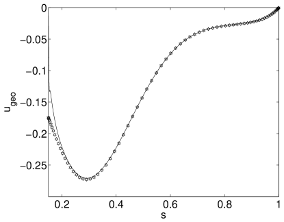
Figure 3: Comparison between numerical (solid line) and analytical (stars) solutions of the geostrophic flow at the equator $u_{\phi}(r,\theta=\frac{\pi}{2})$ for $E=10^{-7}$, $\eta=0.15$, $\tilde{\rho}=10$, $B=1$ and $\lambda=10^{-4}$ without mass contraction.

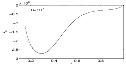
Figure 4: Evolution of the azimuthal velocity $u_{\phi}(r,\theta=\frac{\pi}{2})$ for $\eta=0.15$, $\tilde{\rho}=10$, $E=10^{-7}$, $\lambda=10^{-4}$ and $B=0,10^{4},10^{5},10^{7}$ (downward). The solid line is the numerical solution, the dashed line is the full analytical solution and the two dot lines are the solutions of each flow. The transition is at $B=10^{4}$, the differential rotation is then governed by baroclinicity as shown in Fig. 5. Boundary conditions are no-slip on both sides $r=\eta$ and $r=1$.

3.3 Transition between the two steady flows : the baroclinic flow versus the one induced by mass contraction

Figure 5: Evolution of the differential rotation $\delta\Omega$, the meridional circulation $\psi$ for $\eta=0.15$, $\tilde{\rho}=10$, $E=10^{-7}$, $\lambda=10^{-4}$ and $B=0,10^{4},10^{5},10^{7}$ (downward). In the first column, difference in differential rotation is shown with contours : solid ones are faster than the core and dashed contours are slower than the core. When the spin-up flow dominates the differential rotation we get a fast equator while baroclinicity induces a fast pole. In the second column, meridional circulation is described with dotted lines for clockwise circulation (solid lines for counter-clockwise circulation). Boundary conditions are no-slip on both sides $r=\eta$ and $r=1$.

When gravitational contraction occurs in a baroclinic envelope, two drivings compete : the baroclinic torque and the one induced by mass contraction. To get a global view of this competition we therefore need resorting to numerical solutions. The numerical method is detailed in appendix. The global problem is the superposition of the two flows : the one induced by mass contraction (25) and the baroclinic one (27). Since the system is linear, the full solution is a linear combination of both. At the equator it reads

$$u_{\phi}(r,\theta=\frac{\pi}{2})=\sqrt{\frac{2}{E}}(1-r^{2})^{3/4}\left(\frac{\eta^{2}}{r}-\frac{9}{4\tilde{\rho}\eta}r\right)$$

$$-rB\int_{r}^{1}\frac{n^{2}(r)}{r}dr\;.$$ (33)

From the foregoing equation, we see that the differential rotation is governed by baroclinicity when

$$B\gg E^{-1/2}\;.$$ (34)

It is shown in Fig. 4. However, we also know (from the angular momentum flux balance of a steady flow, see Rieutord 2006a) that the meridional circulation associated with baroclinic flows is ${\cal O}(BE)$, while the meridional circulation of the contraction-induced spin-up is ${\cal O}(1)$. Hence a baroclinic flow completely controls the dynamics as long as $BE\gg 1$. Note that this inequality implies (34) since $E\ll 1$. When the spin-up strengthens, the foregoing inequalities predict an intermediate regime

$$E^{-1/2}\ll B\ll E^{-1}$$ (35)

where the differential rotation is of baroclinic origin ($BE^{1/2}$) but the meridional circulation is driven by contraction ($BE\ll 1$). Finally, when $BE^{1/2}\ll 1$, the flow is fully controlled by the contraction induced spin-up.

This two step transition is confirmed by numerical solutions as illustrated in Fig. 5 and Fig. 6. There, for a given $E$, $B$ is progressively increased and we clearly see the intermediate regime where differential rotation and meridional circulation are of different origin (third row).

Figure 6: $u_{\phi}$ as a function of the normalized radius for $\lambda=10^{-4}$, $\eta=0.15$ and $\tilde{\rho}=10$. The solid line is the numerical solution, dotted lines are the analytical solutions of the spin-up flow and the baroclinic one, the dashed line is the sum of both. Downward : $E=10^{-5},10^{-6},10^{-7}$ and the transition value on the differential rotation is respectively $B=10^{3},3.10^{3},10^{4}$. Beyond this treshold, the baroclinicity governs the differential rotation. Boundary conditions are no-slip on both sides $r=\eta$ and $r=1$. Note that as the Ekman number is getting smaller, the discrepancy between the numerical and the analytical solutions does too.

4 The case of stress-free boundary conditions

The outer layers of the envelope are not rigidly attached to the core. Therefore the use of outer stress-free boundary conditions is more realistic. In this case however, we no longer have access to an analytical expression of the flow in the envelope and have to resort to numerical solutions.

4.1 Scaling the steady mass contraction induced flow

Let us first study the steady solution of the spin-up flow. As shown in Fig. 7, it exhibits the typical cylindrical differential rotation of a dominating mass contraction flow. The equatorial surface region rotates faster than the core and the pole is slower. The meridional circulation displays two cells with a strong Stewartson layer at $s=\eta$ (compared with the previous with no-slip conditions).

Figure 7: Differential rotation and meridional circulation for $E=10^{-7}$, $\eta=0.15$ and $\tilde{\rho}=10$ for an unstratified configuration. For $\delta\Omega$, dashed (resp. solid) lines represent rotation slower (resp. faster) than the core. For $\psi$, dotted (resp. solid) lines are for clockwise (resp. counter-clockwise) circulation. Boundary conditions are no-slip at $r=\eta$ and stress-free at $r=1$.

In Fig. 8, we show the amplitudes of the mass contraction flow at two positions : inside and outside of the tangent cylinder. Since the boundary conditions on the core are no-slip, the flow within the tangent cylinder is expected to be $\mathcal{O}(E^{-1/2})$ according to expression (17). For small cores $\eta=0.15$ or $0.25$, numerical solutions show that the Stewartson layer impacts the interior of the tangent cylinder and that the asymptotic state is reached only at extremely small values of the Ekman number $E\leq 10^{-8}$. When the core is bigger, for instance $\eta=0.5$, the $E^{-1/2}$ scaling inside the tangent cylinder is clearly showing up for all Ekman numbers less than $10^{-5}$.

Outside the tangent cylinder, numerics show that the differential rotation is always $\mathcal{O}(E^{-1})$ when the outer boundary conditions are stress-free. Such an important amplitude indicates that the steady state may not be reached during the contraction phase and may not be studied with linear equations since quadratic terms are expected to be important, namely $\mathcal{O}(\frac{Ro}{E^{2}})$.

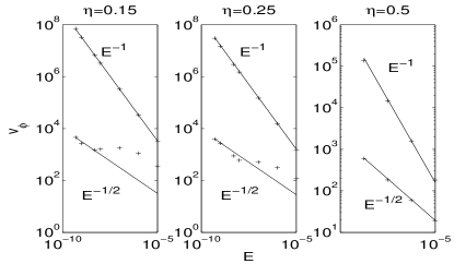
Figure 8: Logarithm of the absolute value of the amplitude of the numerical azimuthal velocity as a function of the logarithm of the Ekman number at $z=0.5$. The left pannel is for $\eta=0.15$, the middle one is for $\eta=0.25$ and the right one for $\eta=0.5$. Inside the tangent cylinder, measures were taken respectively at the points $s=0.1,0.2,0.25$, the azimuthal velocity scales around $E^{-1/2}$. It is proportional to $E^{-1}$ within the envelope $s=0.65$. Note that the azimuthal velocity is mainly negative for small cores and positive for bigger cores like $\eta=0.5$.

4.2 The transient phase

The large amplitude of the steady state outside the tangent cylinder forces us to consider the time evolution of the solution of the mass contraction induced flow. To do so, we solve the set of equations (5) with an order one implicit scheme (Euler’s method) so as to eliminate inertial waves and concentrate on the secular evolution.

In Fig. 9, we plot a proxy of the amplitude of the differential rotation for various Ekman numbers and for no-slip and stress-free outer boundary conditions. With no-slip conditions, we see that the steady spin-up flow is quickly established and justifies the use of a steady solution. On the contrary, the use of outer stress-free boundary conditions leads to a much longer transient flow that lasts more than the typical time scale of the driving by gravitational contraction.

To go further it is interesting to characterize this transient flow with respect to the parameters of the problem. From the numerical solution we find that the transient duration $\tau_{\rm sf}$ scales like

$$\tau_{\text{sf}}\propto RoE^{-0.86}$$ (36)

This scaling of the Ekman number is very close to $E^{-6/7}$ that is reminiscent of one of the scalings of the Stewarston layer in the spherical Couette flow (see Stewartson, 1966). In these layers that surrounds the core along the tangent cylinder, a typical thickness is $E^{2/7}$. This might control the amplitude of the flow outside the tangent cylinder when stress-free outer conditions are met. The analysis of the Stewartson layer associated with this transient flow is difficult and beyond the scope of the present work.

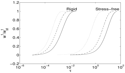
Figure 9: Time evolution of the major component of the azimuthal velocity $w^{l=1}$ normalized by its steady solution $w^{l=1}_{\text{st}}$ as a function of non-dimensional time with $E=10^{-5},10^{-6},10^{-7}$ (respectively the dot, the dashed and the solid line) and $Ro=10^{-6}$ at the radius $r=0.88$. On the left side are the solution with rigid boundary conditions on both sides and on the right side the solutions with stress-free boundary conditions on the outer. In the first case, the steady state is reached in a time smaller the dimensionless time of contraction, while in the second case this time is longer and scale as $E^{-0.86}$.

Another remarkable property of the transient flow is its approximate self-similarity. Its spatial shape remains almost unchanged, while its amplitude grows as time passes. The associated differential rotation is parallel to the $z$-axis as shown in Fig.10. Its amplitude grows according to the time profile displayed in Fig.9. This time dependence can be approximated as

$$\frac{A}{E}(1-e^{-\tau\ln 10/\tau_{\text{sf}}})$$ (37)

where $A$ is a constant of order unity.

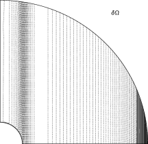
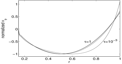
Figure 10: Left: the differential rotation associated with the transient phase of a spin-up induced by mass contraction for $E=10^{-6}$ and $Ro=10^{-6}$ at time $\tau=0.02$. Dashed (resp. solid) lines represent rotation slower (resp. faster) than the core. Right: the profile of the corresponding azimuthal velocity in the equatorial plane as a function of the normalized radius for various times. The curves are scaled by the absolute value of the amplitude at the minimum.

The foregoing result may be translated in the stellar case. It shows that a contracting, fully convective star, may reach a self-similar spin-up flow with cylindrical rotation. Neglecting viscous force (in fact Reynolds stresses), we may expect that substituting $\rho\@vec{v}$ to the foregoing incompressible velocity field, we can get an good representation of the actual flow in a compressible envelope. This is supported by the fact that the geostrophic balance is unchange in this case. Of course, this conjecture has to be verified by the study of the compressible case.

4.3 Transient phase and stratification

During the contraction of a star on the PMS, an initial convective envelope progressively leaves the place to a radiative envelope when the star is massive enough. This radiative envelope is stably stratified and without any extra-forcing from gravitational contraction it would relax to the steady baroclinic state that we mentioned before.

One question is therefore whether the contraction induced spin-up is strong enough to overwhelm the foregoing baroclinic flows that are themselves transient flows. To have an idea of the result we may use the amplitude of a steady baroclinic flows as an upper limit of the actual flows. In this perspective we can use the results of Espinosa Lara & Rieutord (2007) and Espinosa Lara & Rieutord (2013) who showed that the baroclinic flow in a radiative envelope is characterized by a differential rotation that is typically 15% of the bulk rotation. Let us assume that the maximum amplitude of the baroclinic flow reads

$$V_{b}=kV_{\rm eq}$$

where $k\raisebox{-3.01385pt}{$\stackrel{{\scriptstyle<}}{{\,\sim\,}}$}0.2$. During the phase of gravitational contraction the spin-up flow grows according to (37). At some time $\tau_{c}$, the spin-up flow overwhelms the baroclinic flow. At such time we have

$$\frac{A}{E}(1-e^{-\tau_{c}\ln 10/\tau_{\text{sf}}})=\frac{V_{b}}{V_{s}}$$

with $V_{s}\sim R/t_{\rm KH}$, $t_{\rm KH}$ being the Kelvin-Helmholtz time of the star. Hence,

$$\frac{\tau_{c}}{\tau_{\text{sf}}}\sim-\log\left(1-\frac{EV_{b}t_{\rm KH}}{AR}\right)$$ (38)

Using numbers of a typical 3 M_⊙ star on the birthline, we find that

$$\frac{EV_{b}t_{\rm KH}}{AR}=\frac{k}{2A}\frac{\nu GM^{2}}{R^{3}L}\raisebox{-3.01385pt}{$\stackrel{{\scriptstyle<}}{{\,\sim\,}}$}10^{-4}$$

This small ratio indicates that $\tau_{c}\ll\tau_{\text{sf}}$ so that the contraction-induced flow overwhelms the baroclinic one during the linear growth of the transient flow (37). Hence, from (36) we get

$$\tau_{c}\sim\frac{E^{0.14}Ro}{A}\frac{V_{b}t_{\rm KH}}{R}\;.$$

With the definition of $Ro$ and $V_{b}$ it turns out that

$$\tau_{c}\sim\frac{k}{2A}E^{0.14}\;.$$

Because of the very small value of the Ekman number, $\tau_{c}$ is clearly less than unity showing that the spin-up flow will in the end take over the baroclinic flow, likely much before this latter flow can be established.

We verified this conclusion with a numerical simulation integrating the spin-up flow from a pre-existing baroclinic flow driven by a fixed stable stratification. In Fig. 11, we show the time evolution of the azimuthal velocity in the equatorial plane of the star. It describes the transient phase from a steady baroclinic flow to a growing spin-up flow. The transition between the two flows happens between $\tau=10^{-3}$ and $\tau=10^{-2}$. This is less than $\tau_{c}\sim 0.2$ (at $E=10^{-5}$), namely less than our first evaluation obtained by a comparison of the amplitudes of the flows (see Eq. 38). The parameters have been chosen such that $BE\ll 1$ as expected in real situations. $\tau_{c}$ therefore appears as a good indicator of the time needed by spin-up to overwhelm baroclinic flows. Let us finally note that, once the spin-up flow is settled, the flow remains approximately self-similar and this for at least 80% of the Kelvin-Helmholtz time.

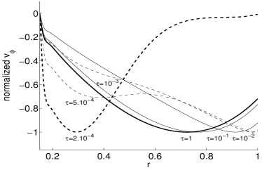
Figure 11: Radial profiles taken at various times of the azimuthal velocity in the equatorial plane of the star for $E=10^{-5}$, $B=10^{2}$, $\epsilon=10^{-7}$, $\lambda=10^{-4}$ and $Ro=10^{-5}$. Profiles are scaled as in Fig. 10. The dimensionless time $\tau$ is specified for each curve. Dashed lines are profiles for baroclinicly dominated dynamics while solid ones are for spin-up dominated dynamics. The dashed bold curve shows the initial profile and the solid bold curve shows the last one.

5 Discussion and conclusions

The gravitational contraction that occurs before or after the main sequence is strongly influencing the rotation rate of the stars and their internal dynamics. In the foregoing study, we have investigated the consequences of the combination of rotation and gravitational contraction with a very simplified model in order to decipher this complicated dynamics and be prepared for the construction of more elaborated models of rotating stars like the ESTER models of Espinosa Lara & Rieutord (2013).

Thus, to the compressible gas of the star, we substituted an incompressible fluid that may also be stably stratified. Schematically, the bell-shaped profile of the star density is replaced by a step function delineating a central core that absorbs matter from the envelope as the star contracts. The size of the core is small and arbitrary. The envelope is either neutrally or stably stratified.

During the contraction on the PMS the stellar envelope of an intermediate-mass star usually passes from a convective to a radiative state. But the radiative state is stably stratified. The combined effect of rotation and stable stratification drives a baroclinic flow that may contest a pre-existing spin-up flow built up during a previous convective phase of the envelope. The question is which of these flows will govern the dynamics of the contracting star and finally determine the initial conditions of the dynamics on the main sequence.

Using our simplified model we compared the strength of these two flows and found that although contraction is slow, the induced spin-up controls the large-scale flows of the outer envelope, namely its differential rotation and meridional circulation. Moreover, our model underlines the role of the outer boundary conditions and shows that with realistic stress-free conditions we should expect an unsteady flow. In addition, it shows that this transient flow keeps a self-similar shape during its growth (if we omit boundary layers).

When the star reaches the main sequence, the contraction turns off and the flows in the envelope relax towards the steady baroclinic flow on the Eddington-Sweet time scale. As far as intermediate-mass stars are concerned, because of their fast rotation, the Eddington-Sweet time scale is close to the Kelvin-Helmholtz one and the transition to the quasi-steady state of the main sequence is quite short (for instance for 7 M_⊙ star, the Eddington-Sweet timescale is 2.8 Myr for a rotation near break-up, to be compared to the 46 Myr of the lifetime of such stars). On the other hand, if for some reason (mainly the combination of magnetic fields and mass loss), the star loses much angular momentum so that $2\Omega\ll N$ at the beginning of the main sequence, then the dynamic state on an outer envelope will be controlled by slowly decaying baroclinic modes excited by the contraction phase. The slow decay may occupy a significant fraction of the main sequence with consequences on the mixing processes.

Back to fluid dynamics, the simple model that we used shows other details on the dynamics of this system, like for instance the shear layer (the Stewartson layer) that circumvent the core on its tangent cylinder. Such a feature is clearly an artefact of the model for stars with no convective cores like PMS stars, but it is certainly an important feature for stars leaving the main sequence where the core contracts and the envelope expands. At the core-envelope interface the build-up of a density jump due to nuclear evolution, combined with rotation, triggers a Stewartson layer on the tangent cylinder of the discontinuity. This layer may indeed explain the efficient transport of angular momentum between the core and envelope of giant or subgiant stars that is needed to explain the rather mild radial differential rotation observed in these stars Deheuvels et al. (2012); Mosser et al. (2012); Eggenberger et al. (2012). Indeed, let us remark that our model shows that there is a tight coupling between the inner part of the tangent cylinder and the core itself. This coupling is essentially a consequence of the Taylor-Proudman theorem that imposes no velocity gradient along the rotation axis (columnar flow). Therefore, the transport of angular momentum between the core and the envelope is much enhanced by the Stewartson layer. Since such a layer has a surface that is $R_{\rm star}/R_{\rm core}$ larger than the surface of the core, we expect that the flux of angular momentum between the core and the envelope will be enhanced by a similar factor (viscosity and velocity gradient being assumed similar) with respect to a 1D shellular profile. Noting that the moment of inertia of the core and of the matter inside its tangent cylinder are not much different, we expect that the Stewartson layer plays a crucial role in the angular momentum exchange between core and envelope and might well be the key feature that reconcile models and observations. It is clear that present 1D models do not take this fluid dynamics feature into account and that the final answer will be given by 2D models incorporating this flow. A dedicated study is clearly needed to give a quantitative estimate of this effect and to offer a new comparison with observations.

Hence, more than the numbers and the applicability to a given object, the foregoing Boussinesq model underlines the main features of the dynamics of a contracting and rotating envelope. It stresses the key role of outer boundary conditions and the various flows that might govern a contracting phase depending on the strength of the stratification. The side effect of the core in this model underlines the role of a Stewartson layer that may appear either after a rapid change in density or in viscosity. The model also stresses the fact that no steady state can be expected as for the interior flows but that these flows may converge towards a universal one when gravitational contraction ceases. The next step of these investigations focusing specifically on stars will be developed with the full physics using the ESTER code of Espinosa Lara & Rieutord (2013).

Appendix A Numerical method

To solve the set of linear equations (12), we discretize the equations using a spectral method. We project the velocity field onto the harmonics spherical base

$$\@vec{u}=\sum\limits_{l=0}^{+\infty}{\sum\limits_{m=-l}^{+l}{u_{m}^{l}\@vec{R}_{l}^{m}+v_{m}^{l}\@vec{S}_{l}^{m}+w_{m}^{l}\@vec{T}_{l}^{m}}}$$ (39)

where

$$\@vec{R}_{l}^{m}=Y_{l}^{m}\@vec{e_{r}},\qquad\@vec{S}_{l}^{m}=\@vec{\nabla}Y_{l}^{m},\qquad\@vec{T}_{l}^{m}=\@vec{\nabla}\times\@vec{R}_{l}^{m}$$ (40)

$Y_{l}^{m}$ are the normalized spherical harmonics, $\@vec{e_{r}}$ is the radial unity vector and $\@vec{\nabla}$ is defined on the unity sphere. We write the temperature perturbation onto the spherical harmonics base too :

$$\theta_{T}=\sum\limits_{l=0}^{+\infty}{\sum\limits_{m=-l}^{+l}t_{m}^{l}Y_{l}^{m}}$$ (41)

We add finally the boundary conditions on this field :

$$\left\{\begin{array}[]{ccl}t_{l}^{\prime}(r=\eta)=0\\ t_{l}(r=1)=0\\ \end{array}\right.$$ (42)

We discretize the radial direction for $r\in[\eta;1]$ onto the Gauss-Lobatto grid associated with the Chebyshev polynomials. Thereby, equations are solved in two dimensions $(r,\theta)$. The system is axisymmetric which implies $m=0$.
The equation of continuity reads

$$v_{m}^{l}=\frac{1}{\Lambda}\frac{1}{r}\frac{\partial}{\partial r}(r^{2}u_{m}^{l})$$ (43)

where $\Lambda=l(l+1)$.
The energy equation reads

$$B\tilde{E}_{T}(r^{2}\frac{\partial^{2}}{\partial r^{2}}t^{l}_{m}+2r\frac{\partial}{\partial r}t^{l}_{m}-\Lambda t^{l}_{m})=n_{T}^{2}(r)r^{2}u^{l}_{m}$$ (44)

The equation of motion is projected onto two directions because equations on $\@vec{R}_{l}^{m}$ and on $\@vec{S}_{l}^{m}$ are redundant.
On $\@vec{R}_{l}^{m}$, it reads

$$A_{l-1}^{l}r^{l-1}\frac{\partial}{\partial r}\left(\frac{u_{m}^{l-1}}{r^{l-2}}\right)+A_{l+1}^{l}r^{-l-2}\frac{\partial}{\partial r}\left(r^{l+3}u_{m}^{l+1}\right)$$

$$+E\Delta_{l}w_{m}^{l}=-\sqrt{\frac{4\pi}{3}}\delta_{l1}(\frac{\eta^{2}}{r^{2}}-r\dot{\omega})$$ (45)

$\delta_{ij}$ is the Kronecker symbol.
On $\@vec{T}_{l}^{m}$, it reads

$$-B_{l-1}^{l}r^{l-1}\frac{\partial}{\partial r}\left(\frac{w_{m}^{l}}{r^{l-1}}\right)-B_{l+1}^{l}r^{-l-2}\frac{\partial}{\partial r}\left(r^{l+2}w_{m}^{l+1}\right)$$

$$-l(l+1)t_{m}^{l}+E\Delta_{l}\Delta_{l}(ru_{m}^{l})=-\sqrt{\frac{16\pi}{5}}n^{2}(r)\delta_{l2}$$ (46)

We note $A_{l-1}^{l}$,$A_{l+1}^{l}$,$B_{l-1}^{l}$ and $B_{l+1}^{l}$ the coupling coefficients.

$$\left\{\begin{array}[]{ccl}A^{l}_{l+1}=\frac{1}{(l+1)}\frac{1}{\sqrt{(2l+1)(2l+3)}}\quad;\quad B^{l}_{l+1}=\frac{l(l+1)(l+2)}{\sqrt{(2l+1)(2l+3)}}\\ A^{l}_{l-1}=\frac{1}{l}\frac{1}{\sqrt{(2l-1)(2l+1)}}\quad;\quad B^{l}_{l-1}=\frac{l(l^{2}-1)}{\sqrt{(2l-1)(2l+1)}}\end{array}\right.$$ (47)

Noting that the forcing implies equatorially symmetric solutions (the resulting differential rotation is equatorially symmetric), the radial functions $w^{l}$ are non-zero only for odd $l$ while $u^{l}$ and $t^{l}$ only for even $l$. The series is therefore $w^{1},u^{2},t^{2},w^{3},\ldots$