$\rm H_{2}^{+}$ in a weak magnetic field

Abstract

The electronic energy of $\rm H_{2}^{+}$ in magnetic fields of up to $B=0.2B_{0}$ (or 4.7 $\times 10^{4}$ Tesla) is investigated. Numerical values of the magnetic susceptibility for both the diamagnetic and paramagnetic contributions are reported for arbitrary orientations of the molecule in the magnetic field. It is shown that both diamagnetic and paramagnetic susceptibilities grow with inclination, while paramagnetic susceptibility is systematically much smaller than the diamagnetic one. Accurate two-dimensional Born-Oppenheimer surfaces are obtained with special trial functions. Using these surfaces, vibrational and rotational states are computed and analysed for the isotopologues $\rm H_{2}^{+}$ and $\rm D_{2}^{+}$.

Keywords: Variational method, weak magnetic fields, magnetic susceptibility, rovibrational states

1 Introduction

Since the pioneering work of de Melo et al. [1] on the molecular ion $\rm H_{2}^{+}$ in strong magnetic fields, $B\geq B_{0}$ ($B_{0}=2.35\times 10^{9}$ Gauss $=2.35\times 10^{5}$ T), many studies have been conducted for this system under such conditions (see for example [2]-[10] and references therein) where the electronic energy of the ground and first excited states as well as some rotation-vibrational states have been studied. $\rm H_{2}^{+}$ has been used as a test system for the investigation of the validity of approximations commonly made in field-free molecular physics, such as the Born-Oppenheimer approximation [12, 13]. Though $\rm H_{2}^{+}$ can be considered a benchmark molecule for the development of appropriate theoretical methods for the accurate computation of molecular structure and properties in magnetic fields that may be extended to more complex systems [7, 14, 15, 16], only few studies have been reported in the range of small fields ($0\leq B\leq B_{0}$) [18, 17], where electronic energies of the ground state and physical features such as a qualitative evolution of the rotational levels as function of the field are presented.

The goal of the present study is to investigate the electronic ground state of the molecular system $\rm H_{2}^{+}$ placed in a weak magnetic field, $B\leq 0.2B_{0}$. Overall in this domain of field strength, the effects of the magnetic field cannot be treated accurately via perturbation theory. In the first part of the present work we use physically motivated, specially tailored trial functions [5, 6, 7] to obtain sufficiently accurate estimates of the electronic energy over a range of field strengths up to $B=B_{0}$ and different inclinations of the molecular axis with respect to the field direction. In the second part we investigate the vibrational and rotational structure of $\rm H_{2}^{+}$ and $\rm D_{2}^{+}$ in the external magnetic field.

2 Hamiltonian

We consider a homonuclear molecular ion formed by two nuclei of charge $q$ separated by a distance $R$, and one electron $e$ placed in a uniform magnetic field $\vec{B}$ oriented along the $z$-axis. The reference point for coordinates is chosen to be at the midpoint of the line connecting the nuclei which in turn forms an angle $\theta$ with respect to the magnetic field direction (see Figure 1).

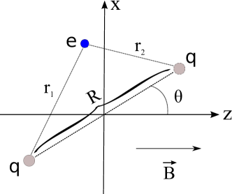
Figure 1: The homonuclear molecular ion consisting of two centers of charge $q$ separated by a relative distance $R$, and one electron $e$. The system is placed in a uniform magnetic field $\vec{B}$ along $z$-axis.

In the framework of non-relativistic quantum mechanics, i.e. neglecting spin interactions, following pseudoseparation of the center of mass motion  and resorting to the Born-Oppenheimer approximation of order zero, i.e. neglecting terms of order smaller than $1/\cal{M}$ ($\cal{M}$ is the total mass of the system), the Hamiltonian that describes the system is given by

$$\hat{\cal H}=\frac{2}{M_{s}}\left[\hat{P}_{R}-\frac{q}{2}\vec{\cal A}_{R}\right]^{2}+\frac{1}{2m_{e}}\left[\hat{p}-e\vec{A}_{e}\right]^{2}+\frac{q^{2}}{R}+qe\left(\frac{1}{r_{1}}+\frac{1}{r_{2}}\right),$$ (1)

where $M_{s}$ is the total mass of the nuclei, $q$ is the nuclear charge, $\hat{P}_{R}=-i\hbar\nabla_{R}$ is the momentum operator and $\vec{A}_{R}$ ($\vec{A}_{R}=\frac{1}{2}\,\vec{B}\times\vec{R}$) is the vector potential for the relative motion ${\vec{R}}$ of the nuclei; $e$ and $m_{e}$ are the electronic charge and mass, respectively; $\hat{p}=-i\hbar\nabla_{r}$ and $\vec{A}_{e}$ are the momentum operator and vector potential for the electron which is at the position $\vec{r}=(x,y,z)$; $r_{1}$ and $r_{2}$ are the distances between the electron and each of the nuclei. In the Hamiltonian (1) the first term is the kinetic energy of the nuclear relative motion in a magnetic field; the remaining terms correspond to the electronic Hamiltonian, written in the Born-Oppenheimer approximation of zero order. In the remainder of this article, atomic units shall be used, i.e. distances are measured in Bohr, $a_{0}=1\,$ a.u., energies in Hartrees, $E_{h}=1\,$ a.u. and $\hbar=|e|=m_{e}=1$.

3 Solving the electronic Schrödinger equation

To solve the electronic Schrödinger equation an appropriate gauge for $\vec{A}_{e}$ must be chosen. Though the problem is in principle gauge invariant this is not the case if the equation is solved approximately [17, 19, 8]. We have therefore adopted the strategy of introducing a variational parameter, $\xi$, in the definition of the gauge which is then varied together with the variational parameters of the wave function. For a magnetic field directed along the $z$-axis $\vec{B}=B\hat{z}$, a suitable vector potential is

$$\vec{A}_{e}=B\left[(\xi-1)y,\xi x,0\right],$$ (2)

where $\xi$ is the parameter of the family of Coulomb gauges. With $\xi=0$ the Landau gauge is obtained, while $\xi=1/2$ corresponds to the symmetric gauge. Substituting (2) into (1) we obtain the electronic Hamiltonian (the last three terms in (1)) in the form

$$\hat{\cal H}_{elec}= - \frac{1}{2}\nabla^{2}-iB\left[(\xi-1)y\partial_{x}+\xi x\partial_{y}\right]$$

$$+ \frac{1}{2}B^{2}\left[\xi^{2}x^{2}+(1-\xi)^{2}y^{2}\right]+\frac{q^{2}}{R}-\left(\frac{1}{r_{1}}+\frac{1}{r_{2}}\right).$$

As usual, in (3) the contribution to the energy due to the Coulomb interaction between the nuclei, i.e. $q^{2}/R$, is treated classically. Hence, $R$ is considered an external parameter.

3.1 Trial functions

A set of physically adequate real trial functions introduced in [5, 6, 7] are used to calculate the total energy of the electronic Hamiltonian (3). Thus, the trial function employed in the present study is a linear superposition of three particular functions,

$$\Psi=A_{1}\Psi_{1}+A_{2}\Psi_{2}+A_{3}\Psi_{3}\,,$$ (4)

where

$$\Psi_{1}=\ e^{-\alpha_{1}(r_{1}+r_{2})}e^{-B[\beta_{1x}\xi x^{2}+\beta_{1y}(1-\xi)y^{2}]}\,,$$ (5)

is a Heitler-London type function,

$$\Psi_{2}=\left(e^{-\alpha_{2}r_{1}}+e^{-\alpha_{2}r_{2}}\right)e^{-B[\beta_{2x}\xi x^{2}+\beta_{2y}(1-\xi)y^{2}]}\,,$$ (6)

is a Hund-Mulliken type function, and

$$\Psi_{3}=\left(e^{-\alpha_{3}r_{1}-\alpha_{4}r_{2}}+e^{-\alpha_{3}r_{2}-\alpha_{4}r_{1}}\right)e^{-B[\beta_{3x}\xi x^{2}+\beta_{3y}(1-\xi)y^{2}]}\,,$$ (7)

is a Guillemin-Zener type function, all multiplied with exponential terms that correspond to the lowest Landau orbital.

Without loss of generality one of the linear parameters $A_{1,2,3}$ may be set equal to one, hence the trial function consists of 13 variational parameters. For the parallel configuration the parameters are not independent and must obey the symmetry relations $\beta_{1x}=\beta_{1y}$, $\beta_{2x}=\beta_{2y}$ and $\beta_{3x}=\beta_{3y}$, reducing the number of variational parameters to ten. The trial function (4) defined in this way is expected to provide an accurate approximation to the exact electronic wave function of the ground state of molecular ion $\rm H_{2}^{+}$ for a large variety of strengths and inclinations of the magnetic field.

Calculations are performed using the minimization package MINUIT from CERN-LIB. Numerical integrations were done with a relative accuracy of $\sim 10^{-6}$ using the adaptive NAG-LIB (D01FCF) routine.

3.2 Results

Using the trial function (5) presented in Section 3.1, two-dimensional potential energy surfaces of the electronic energy have been obtained variationally as function of the internuclear distance, $R$, and the inclination $\theta$ (see Figure 1).

As examples we show in Figures 2 and 3 sections of the potential surface at different inclinations, $\theta=0^{\circ},45^{\circ}$ and $90^{\circ}$, for $B=0.2B_{0}$ and $B=0.5B_{0}$.

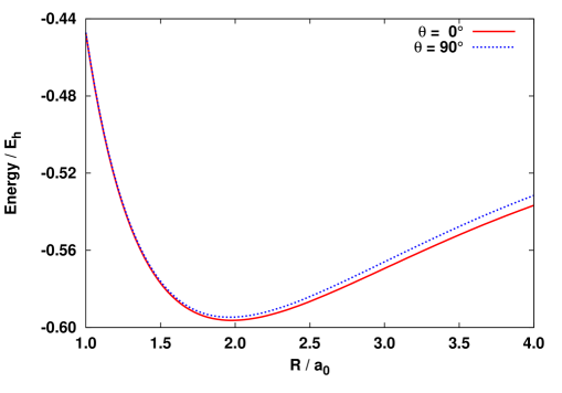
Figure 2: Potential energy curves for $\rm H_{2}^{+}$ in an external field of $B=0.2B_{0}$ at parallel ($\theta=0^{\circ}$) and perpendicular ($\theta=90^{\circ}$) orientations.

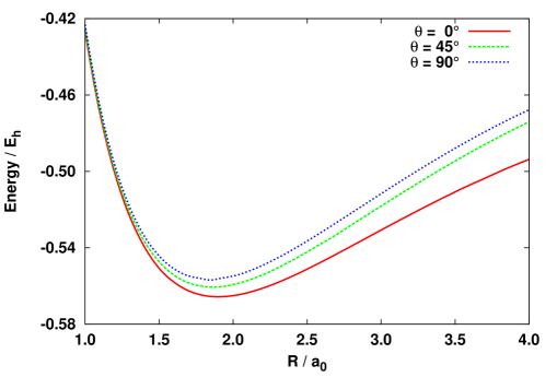
Figure 3: Potential energy curves for $\rm H_{2}^{+}$ in an external field of $B=0.5B_{0}$ at orientation angles $\theta=0^{\circ}$, $\theta=45^{\circ}$ and $\theta=90^{\circ}$.

The most stable configuration is achieved for parallel orientation of the molecule, which is a well known result for $B\geq 10^{5}\,$T [7]. At perpendicular orientation an energy ridge shows up which can be interpreted as barrier of a hindered rotation. This fact is shown in more detail in Figure 4 where the electronic energy is plotted as function of the inclination for the fields $B=0.1\,B_{0}$ and $0.2\,B_{0}$. It is worth noting that at large distance $R\gg R_{eq}$, when the system separates to a proton and a hydrogen atom, the potential surface exhibits a relative maximum at $\sim 45^{\circ}$ inclination which is due to interaction of the proton charge with the quadrupole moment of the atom [20]. As the sign of the interaction term is angular dependent, a barrier is built up as the molecule is oriented from parallel towards perpendicular configuration [7]. With increasing field strength and inclination, the internuclear distance at equilibrium becomes smaller while the rotational barrier is increased. Data are presented in Table 1. In Figure 5 the equilibrium distance $R_{eq}(B,\theta)$ is plotted as a function of $\theta$ for the field strengths $B=0.1\,B_{0}$ and $0.2\,B_{0}$.

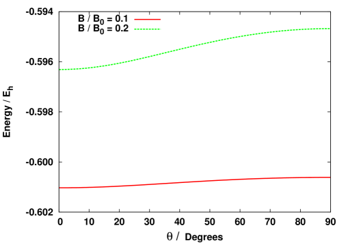
Figure 4: Electronic energy at equilibrium distance as function of inclination for $\rm H_{2}^{+}$ in an external field of $B=0.1\,B_{0}$ and $0.2\,B_{0}$.

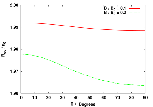
Figure 5: Equilibrium distance in a.u. of $\rm H_{2}^{+}$ in an external field as function of the inclination angle and field strengths of $B=0.1\,B_{0}$ and $0.2\,B_{0}$.

Table 1: Total energy at equilibrium distance as function of the field strength and inclination.

$B/B_{0}$	$\theta$	$R_{eq}/a_{0}$	Energy/$E_{h}$	$B/B_{0}$	$\theta$	$R_{eq}/a_{0}$	Energy/$E_{h}$
$0$	$-$	1.9971	-0.602625
$0.1$	$0^{\circ}$	1.9920	-0.601029	$0.6$	$0^{\circ}$	1.8705	-0.550864
	$45^{\circ}$	1.9897	-0.600785		$45^{\circ}$	1.8201	-0.543923
	$90^{\circ}$	1.9882	-0.600613		$90^{\circ}$	1.7968	-0.539131
$0.2$	$0^{\circ}$	1.9786	-0.596311	$0.7$	$0^{\circ}$	1.8399	-0.534186
	$45^{\circ}$	1.9687	-0.595361		$45^{\circ}$	1.7800	-0.525296
	$90^{\circ}$	1.9637	-0.594678		$90^{\circ}$	1.7535	-0.519216
$0.3$	$0^{\circ}$	1.9566	-0.588667	$0.8$	$0^{\circ}$	1.8096	-0.515853
	$45^{\circ}$	1.9379	-0.586615		$45^{\circ}$	1.7411	-0.504917
	$90^{\circ}$	1.9283	-0.585161		$90^{\circ}$	1.7112	-0.497503
$0.4$	$0^{\circ}$	1.9301	-0.578360	$0.9$	$0^{\circ}$	1.7799	-0.496041
	$45^{\circ}$	1.9013	-0.574889		$45^{\circ}$	1.7027	-0.482994
	$90^{\circ}$	1.8862	-0.572447		$90^{\circ}$	1.6721	-0.474219
$0.5$	$0^{\circ}$	1.9019	-0.565667	$1.0$	$0^{\circ}$	1.7563	-0.474937
	$45^{\circ}$	1.8610	-0.560550		$45^{\circ}$	1.6687	-0.459670
	$90^{\circ}$	1.8413	-0.556976		$90^{\circ}$	1.6348	-0.449532

3.3 Magnetic Susceptibility

An important quantity that describes the response of the molecular system with respect to the external field is the magnetic susceptibility. It is defined via a Taylor expansion of the electronic energy in powers of the magnetic field $B$

$$E(\vec{B})=E(0)-\sum_{\alpha}c_{\alpha}B_{\alpha}-\frac{1}{2}\sum_{\alpha\beta}\chi_{\alpha\beta}B_{\alpha}B_{\beta}+\ldots$$ (8)

For the electronic ground state, when the spin contributions are neglected, the first coefficient, $c_{\alpha}$, vanishes. The coefficient tensor $\chi_{\alpha\beta}$ is the magnetic susceptibility. The response of a molecule to an external magnetic field leads to a classification into two types (see for example [21]): diamagnetic and paramagnetic.

In the electronic Hamiltonian (3) there are two terms containing the magnetic field, $B$, a linear and a quadratic one. Correspondingly, there are two contributions to the susceptibility: a paramagnetic contribution originating from the linear term of the Hamiltonian when treated by second order perturbation theory in $B$, and a diamagnetic contribution coming from the quadratic term in the first order in perturbation theory in $B$.

At first, let us proceed to the diamagnetic susceptibility. The diamagnetic susceptibility term $\chi^{d}$ can be expressed as the expectation value with respect to the field-free wavefunction at equilibrium distance. Thus, in the symmetric gauge, $\vec{A}_{e}=\frac{1}{2}\vec{B}\times\vec{\rm r}$, the expression of the diamagnetic susceptibility tensor is

$$\chi_{\alpha\beta}^{d}=-\frac{1}{4}\left[\langle\vec{r}^{2}\rangle\delta_{\alpha\beta}-\langle r_{\alpha}r_{\beta}\rangle\right],$$ (9)

where $\vec{r}=(x,y,z)$ is the position vector of the electron and $r_{\alpha}$, $\alpha=1,2,3$, its components. If the magnetic field direction is chosen along the $z$-axis, $\vec{B}=B\hat{z}$, the tensor $\chi^{d}$ contains a single non-zero component, $\chi_{zz}^{d}\equiv\chi^{d}$,

$$\chi^{d}=-\frac{1}{4}\langle\rho^{2}\rangle=-\frac{1}{4}\left[\langle x^{2}\rangle+\langle y^{2}\rangle\right]\,.$$ (10)

Let us now consider the molecule in the $x$-$z$ plane (it can be regarded as the definition of the $x$-direction). For different orientations of the molecule with respect to the $z$-axis, the expectation values change according to a rotation by the angle $\theta$ around the $y$-axis ($x\to x\cos\theta+z\sin\theta$, $y\to y$, $z\to z\cos\theta-x\sin\theta$)

$$\chi^{d}=-\frac{1}{4}\left[\langle x^{2}\rangle_{0}\left(1+\cos^{2}\theta\right)+\langle z^{2}\rangle_{0}\sin^{2}\theta\right],$$ (11)

where $\langle x^{2}\rangle_{0}$ and $\langle z^{2}\rangle_{0}$ are the expectation values at zero inclination, and where we have used the fact that $\langle x^{2}\rangle_{0}=\langle y^{2}\rangle_{0}$ and $\langle xz\rangle_{0}=0$. In Table 2, the numerical values of the expectation values of the squares of the components of the position vector of the electron, and the diamagnetic susceptibility, $\chi^{d}$, are presented, at equilibrium distance, as function of $\theta$ and compared with results obtained by Hegstrom [26] for parallel and perpendicular orientations.

Table 2: Expectation values of $x^{2}$, $y^{2}$ and $z^{2}$ for $B=0$, evaluated at the equilibrium distance $R=R_{eq}=1.9971\,a_{0}$, and diamagnetic, paramagnetic and total susceptibility ($\chi^{d}$, $\chi^{p}$, $\chi$) as function of $\theta$. $\chi^{p}$, obtained as $\chi^{p}=\chi-\chi^{d}$, is included for convenience.

$\theta$	$\langle x^{2}\rangle$	$\langle y^{2}\rangle$	$\langle z^{2}\rangle$	$\chi^{d}$	$\chi^{p}$	$\chi$
$0^{\circ}$	0.64036	0.64036	1.11131	-0.32018	0.00000	-0.32018
				-0.3209[26]	—	-0.3209
$15^{\circ}$	0.67192	0.64037	1.07976	-0.32807	0.00022	-0.32785
$30^{\circ}$	0.75810	0.64035	0.99359	-0.34961	0.00216	-0.34745
$45^{\circ}$	0.87583	0.64040	0.87583	-0.37906	0.00992	-0.36914
$60^{\circ}$	0.99357	0.64038	0.75811	-0.40849	0.02062	-0.38787
$75^{\circ}$	1.07971	0.64042	0.67196	-0.43003	0.03090	-0.39913
$90^{\circ}$	1.11125	0.64041	0.64041	-0.43792	0.03447	-0.40345
				-0.4382[26]	0.0378[26]	-0.4004[26]

For strong fields, higher powers of $B$ might need to be considered in the expansion (8). With our variational method, evaluation of higher order terms is straightforward as the trial functions depend parametrically on the field strength. To this end we define the function $X(\vec{B})=-\langle\rho^{2}\rangle_{B}/4$, where the expectation value is taken with the optimized, $B$-dependent trial function. In the limiting case when $B\to 0$, the diamagnetic susceptibility is recovered, $X(\vec{B})\to\chi^{d}$. Numerical results of $X(\vec{B})$ were obtained at the equilibrium distances for $B=0.0,0.01,\dots 0.2\,B_{0}$ and $\theta=0^{\circ},15^{\circ},\dots 90^{\circ}$ and fitted ($rms=1.6\times 10^{-4}$) to a simple functional form of the field strength $B$ and inclination $\theta$,

$$X_{a}(\vec{B})= -0.43795+0.013498B+0.37103B^{2}$$

$$+\left(0.11774-0.01577B-0.141B^{2}\right)\cos^{2}\theta.$$

This surface is plotted in Figure 6,

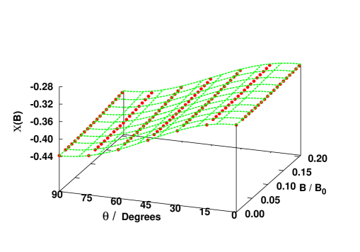
Figure 6: Numerical values of the $X(B)=-\langle\rho^{2}\rangle_{B}/4$ (red dots) and the surface generated by (3.3) as function of the magnetic field $\vec{B}$. The angle $\theta$ is the orientation of the molecule with respect to the field orientation.

while cuts at constant orientation angles are presented in Figure 7.

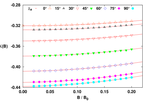
Figure 7: Numerical values of the $X(B)=-\langle\rho^{2}\rangle_{B}/4$ and cuts of model (3.3), $X_{a}$, as function of the field strength $B$, for different given orientations.

It can be seen that the $X(\vec{B})$ is a smooth function of the orientation angle, $\theta$, and the field strength, $B$, and tends to the magnetic susceptibility $X(\vec{B})\to\chi^{d}$ as the field tends to zero. The points on the ordinate represent the value of the magnetic susceptibility $\chi^{d}$ for various orientations and agree with the corresponding data obtained from the model (3.3), within the accuracy. At weak fields $\lesssim$ $0.04\,B_{0}$, $X$ is close to $\chi^{d}$ as given by (11). It indicates that perturbation theory in $B$ can be applied and can provide sufficiently accurate results. Eventually the diamagnetic susceptibility can be given ($rms=1.6\times 10^{-4}$) as

$$\chi^{d}=-0.43795+0.11774\cos^{2}\theta\,,$$ (13)

(c.f. (3.3)). Turning now to the total susceptibility $\chi$. In principle, it can be obtained directly using the Taylor expansion (8) of the energy potential curve $E=E(B,R,\theta)$ for fixed $\theta$ in powers of $B$, but taken into account that the equilibrium distance $R_{eq}(B,\theta)$ evolves in $B$. It is a quite complicated procedure. It is much easier to calculate numerically the energy evolution with $B$ at minimum of the energy potential curve at fixed inclination. Then interpolate this curve $E(B)$ near the origin, $B=0$ using a polynomial of finite degree in $B$. The total susceptibility $\chi$ will be related to the coefficient $E^{(2)}$ in front of the $B^{2}$ term. Numerical values of the total susceptibility, defined as $\chi=-2E^{(2)}$ for different inclination $\theta$, are presented in Table 2. They can be fitted accurately ($rms=3.45\times 10^{-4}$) to the following expression,

$$\chi=-0.41067+0.08260\cos^{2}{\theta}+0.007620\cos^{2}{2\theta}\,.$$ (14)

Hence, for arbitrary inclination, the diamagnetic and total susceptibility can be obtained using the expressions (13) and (14). Finally, the paramagnetic contribution to the susceptibility can be evaluated as the difference $\chi^{p}=\chi-\chi^{d}$, see data in Table 2. In general, the paramagnetic susceptibility is much smaller that the diamagnetic part. It grows with inclination.

Concerning our statement that standard first order perturbation theory based on the field-free $H^{(0)}$ problem should be applicable up to $B\approx 0.04\,B_{0}$, we may now add that at least 92% of the total susceptibility is recovered in this way. The energy correction quadratic in $B$ is accurate to $\sim 6\times 10^{-5}\,E_{h}$.

4 Solving the nuclear Schrödinger equation

Substituting in the Hamiltonian (1) the electronic part (last three terms) by the potential energy surface, $\tilde{V}(R,\theta)$, we obtain the nuclear Hamiltonian. In the symmetric gauge, it can be written as

$$\hat{\cal H}_{nuc}=\frac{2}{M_{s}}\hat{P}_{R}^{2}-\frac{1}{M_{s}}\vec{B}\cdot\hat{L}_{R}+\frac{1}{8M_{s}}\left[B^{2}\vec{R}^{2}-(\vec{B}\cdot\vec{R})^{2}\right]\ +\tilde{V}(R,\theta),$$ (15)

where $\hat{L}_{R}=\vec{R}\times\hat{P}_{R}$ is the angular momentum operator of the molecular frame. Transforming the Hamiltonian in spherical coordinates yields

$$\hat{\cal H}_{nuc}=-\frac{2}{M_{s}}\frac{1}{R}\frac{\partial^{2}}{\partial R^{2}}R+\frac{2}{M_{s}R^{2}}\hat{L}_{R}^{2}-\frac{1}{M_{s}}B\hat{L}_{z}+\frac{1}{8M_{s}}B^{2}R^{2}\sin^{2}{\theta}+\tilde{V}(R,\theta),$$ (16)

where $\hat{L}_{z}$ is the projection of angular momentum along $z$-axis and $\theta$ the angle between the molecular and the $z$-axis.

We have solved the nuclear Schrödinger equation with Hamiltonian (16) numerically. To this end the Hamiltonian is divided in the two separate terms

$$\hat{\cal H}_{1}=-\frac{2}{M_{s}}\frac{1}{R}\frac{\partial^{2}}{\partial R^{2}}R+\tilde{V}(R,\theta^{\prime})+\frac{1}{8M_{s}}B^{2}R^{2}\sin^{2}{\theta^{\prime}}$$ (17)

and

$$\hat{\cal H}_{2}=\frac{2}{M_{s}R^{2}}\hat{L}_{R}^{2}-\frac{1}{M_{s}}B\hat{L}_{z}+\frac{1}{8M_{s}}B^{2}R^{2}\left(\sin^{2}\theta-\sin^{2}\theta^{\prime}\right)+\tilde{V}(R,\theta)-\tilde{V}(R,\theta^{\prime})$$ (18)

which roughly correspond to a vibrational part of the molecule with reference orientation angle $\theta^{\prime}$, and a rotational part. The rovibrational wave function is then expanded in terms of vibrational and rotational basis functions as

$$\Psi(R,\theta,\phi)=\sum_{v,L}c_{v,L}\frac{\xi_{v}(R;\underline{\theta}^{\prime})}{R}Y_{L}^{M}(\theta,\phi)$$ (19)

where $\xi_{v}(R;\underline{\theta}^{\prime})$ are solutions of (17), obtained by numerical integration using the renormalized Numerov algorithm, and $Y_{L}^{M}(\theta,\phi)$ are spherical harmonics. The matrix elements of Hamiltonian (16) in this basis are

$$\left\langle v^{\prime}L^{\prime}M|\hat{\cal H}_{nuc}|vLM\right\rangle = E_{v}(\theta^{\prime})\delta_{L^{\prime}L}\delta_{v^{\prime}v}+\frac{2}{M_{s}}\left\langle v^{\prime}|\frac{1}{R^{2}}|v\right\rangle L(L+1)\delta_{L^{\prime}L}$$

$$- \frac{BM}{M_{s}}\delta_{L^{\prime}L}\delta_{v^{\prime}v}$$

$$+ \frac{B^{2}}{8M_{s}}\left\langle L^{\prime}M|\sin^{2}\theta-\sin^{2}\theta^{\prime}|LM\right\rangle\left\langle v^{\prime}|R^{2}|v\right\rangle$$

$$+ \left\langle v^{\prime}L^{\prime}M|\tilde{V}(R,\theta)-\tilde{V}(R,\theta^{\prime})|vLM\right\rangle$$

with $E_{v}(\theta^{\prime})$ the eigenvalue of the vibrational operator (17). To evaluate these matrix elements, the potential $\tilde{V}(R,\theta)$ is presented as that of a hindered rotator,

$$\tilde{V}(R,\theta) = \tilde{V}(R,0)+\sum_{n}\frac{V_{90,n}(R)}{2}\left[1-\cos(2n\theta)\right]$$ (21)

$$\approx \tilde{V}(R,0)+V_{90}(R)\sin^{2}\theta$$

$V_{90}(R)=\tilde{V}(R,90)-\tilde{V}(R,0)$ is the barrier height for a given value of $R$.

Limitation of the above expansion to just one term is a good approximation of the potential at the field strengths considered in the present work, as we have verified numerically. The $rms$ values for fits of $V(R_{eq},\theta)$, using increments $\Delta\theta=5^{\circ}$, are $rms=7.98\times 10^{-5}$ and $rms=3.66\times 10^{-6}$ for the one and two-term approximations and $B=0.2B_{0}$. For $B=0.1B_{0}$ the fitting error is reduced by a factor of four, approximately. Figure 8 shows the performance of the two approximations.

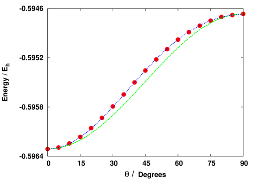
Figure 8: Comparison between the hindered rotor approximation at first order (green line) and second order (blue) with a cut of the potential energy surface at $R_{eq}=1.9788\,a_{0}$, the equilibrium distance when molecule is oriented parallel to the field, for $B=0.2B_{0}$.

The one-term approximation thus represents the potential energy surface to within the accuracy of the raw data of the electronic energy. An appealing feature is that just two slices, at $\theta=0^{\circ}$ and $\theta=90^{\circ}$ of the surface are needed explicitly. Within the one-term approximation and choosing the reference orientation $\theta^{\prime}=0$, the matrix elements can be evaluated readily as 

$$\left\langle v^{\prime}L^{\prime}M|\hat{\cal H}_{nuc}|vLM\right\rangle = E_{v}\delta_{L^{\prime}L}\delta_{v^{\prime}v}+\frac{2}{M_{s}}\left\langle v^{\prime}|\frac{1}{R^{2}}|v\right\rangle L(L+1)\delta_{L^{\prime}L}$$ (26)

$$- \frac{BM}{M_{s}}\delta_{L^{\prime}L}\delta_{v^{\prime}v}$$

$$+ \left[\frac{B^{2}}{12M_{s}}\langle v^{\prime}|R^{2}|v\rangle+\frac{2}{3}\langle v^{\prime}|V_{90}(R)|v\rangle\right]\delta_{L^{\prime}L}$$

$$- \left[\frac{B^{2}}{12M_{s}}\langle v^{\prime}|R^{2}|v\rangle+\frac{2}{3}\langle v^{\prime}|V_{90}(R)|v\rangle\right]$$

$$\times (-1)^{M}\sqrt{(2L^{\prime}+1)(2L+1)}$$

$$\times \left(\begin{array}[]{ccc}L&2&L^{\prime}\\ 0&0&0\end{array}\right)\left(\begin{array}[]{ccc}L&2&L^{\prime}\\ M&0&-M\end{array}\right)$$

The terms in parentheses are Wigner $3j$-symbols. The matrix (26) is diagonal in $M$ as expected, since $M$ is an exact quantum number. $L$-functions are coupled in steps of 2, conserving parity.

4.1 Results

For the isotopologues $\rm H_{2}^{+}$ and $\rm D_{2}^{+}$ we have computed the rovibrational eigenvalues of the nuclear Hamiltonian for the four lowest vibrational states and rotational excitation up to $L=5$ with respect to the field-free case. Two levels of approximation are considered: a simplified model in which only the diagonal terms with respect to the vibrational basis are retained, and a second model which consists in diagonalizing the Hamiltonian (26) in the full basis. These data are presented in Tables 4.1 to 4.1. The results obtained at the two levels of approximation agree to within $10^{-5}\,E_{h}$.

Table 3: Rotational energy levels of $\rm H_{2}^{+}$ in presence of a uniform magnetic field $B$ for the vibrational state $v=0$. The pure vibrational state ($L=0$ in the field-free case) is forbidden but shown here nevertheless as it corresponds to the origin of the rotational band. In the simple model 1, terms off-diagonal in $v$ are neglected. In model 2, the full matrix (26) is diagonalized.

$L$	Energy/$E_{h}$	$M$	$\pi$	Energy/$E_{h}$
	$B=0.0$			$B=0.1$		$B=0.2$
				model 1	model 2	model 1	model 2
		-5	1	-0.591213	-0.591278	-0.584991	-0.585024
		5	1	-0.591485	-0.591550	-0.585535	-0.585568
		-4	-1	-0.591308	-0.591375	-0.585330	-0.585371
		4	-1	-0.591525	-0.591593	-0.585765	-0.585807
		-3	1	-0.591386	-0.591455	-0.585581	-0.585628
$L=5$	-0.593475	3	1	-0.591550	-0.591618	-0.585907	-0.585955
		-2	-1	-0.591449	-0.591520	-0.585769	-0.585822
		2	-1	-0.591558	-0.591629	-0.585987	-0.586040
		-1	1	-0.591498	-0.591569	-0.585902	-0.585957
		1	1	-0.591553	-0.591623	-0.586011	-0.586066
		0	-1	-0.591532	-0.591604	-0.585982	-0.586038
		-3	1	-0.593689	-0.593697	-0.587619	-0.587621
		3	1	-0.593852	-0.593860	-0.587946	-0.587948
		-2	-1	-0.593814	-0.593823	-0.588093	-0.588098
$L=3$	-0.595803	2	-1	-0.593923	-0.593932	-0.588311	-0.588315
		-1	1	-0.593894	-0.593904	-0.588257	-0.588265
		1	1	-0.593948	-0.593958	-0.588366	-0.588374
		0	-1	-0.593938	-0.593948	-0.588408	-0.588417
		-1	1	-0.595124	-0.595124	-0.589358	-0.589364
$L=1$	-0.597120	1	1	-0.595178	-0.595178	-0.589467	-0.589473
		0	-1	-0.595327	-0.595327	-0.590107	-0.590109
$L=0$	-0.597386	0	-1	-0.595492	-0.595492	-0.590136	-0.590139

Table 4: Rotational energy levels of $\rm H_{2}^{+}$ in presence of a uniform magnetic field $B$ for the vibrational state $v=1$. See Caption of Table 4.1 for explications.

Table 5: Rotational energy levels of $\rm H_{2}^{+}$ in presence of a uniform magnetic field $B$ for the vibrational state $v=2$. The pure vibrational state ($L=0$ in the field-free case) is forbidden but shown here nevertheless as it corresponds to the origin of the rotational band See Caption of Table 4.1 for explications.

Table 6: Rotational energy levels of $\rm H_{2}^{+}$ in presence of a uniform magnetic field $B$ for the vibrational state $v=3$. See Caption of Table 4.1 for explications.

Table 7: Rotational energy levels of $\rm D_{2}^{+}$ in presence of a uniform magnetic field $B$ for the vibrational state $v=0$. See Caption of Table 4.1 for explications.

Table 8: Rotational energy levels of $\rm D_{2}^{+}$ in presence of a uniform magnetic field $B$ for the vibrational state $v=1$. See Caption of Table 4.1 for explications.

Table 9: Rotational energy levels of $\rm D_{2}^{+}$ in presence of a uniform magnetic field $B$ for the vibrational state $v=2$. See Caption of Table 4.1 for explications.

Table 10: Rotational energy levels of $\rm D_{2}^{+}$ in presence of a uniform magnetic field $B$ for the vibrational state $v=3$. See Caption of Table 4.1 for explications.

If spin effects are neglected, rovibrational states of $\rm H_{2}^{+}$ in a magnetic field can be classified in terms of three quantum numbers: the vibrational quantum number, $\nu$, the projection of the angular momentum of the molecular frame on the field axis, $M$, and the $z$-parity, $\pi$. The latter quantum number is due to the fact that positive and negative $z$-directions of the field are equivalent. If the wave function is reflected at the plane $z=0$, $\theta$ is mapped to $\pi-\theta$ and $Y_{L}^{M}(\pi-\theta,\phi)=(-1)^{L+M}Y_{L}^{M}(\theta,\phi)$. The $z$-parity of the state is thus $\pi=(-1)^{L+M}$. The nuclear wave function of a system of two fermions must be antisymmetric with respect to an exchange of the nuclei. The vibrational part of the wave function is symmetric for even vibrational quanta, $v=0,2,\dots$ and antisymmetric for odd, $v=1,3,\dots$. The symmetry of the rotational part can be derived from the properties of the spherical harmonics with respect to inversion, ($\theta,\phi\rightarrow\theta+\pi,\phi+\pi$), $Y_{L}^{M}(\theta+\pi,\phi+\pi)=(-1)^{L}Y_{L}^{M}(\theta,\phi)$. Hence for even $v$ the rotational functions must have odd parity, while for odd $v$ they must have even parity, just as in the field-free case. The expression for the $z$-parity is

$$\pi=(-1)^{M+v+1}=\left\{\begin{array}[]{rl}-(-1)^{M}&{\rm for}\leavevmode\nobreak\ v\leavevmode\nobreak\ {\rm even}\\ (-1)^{M}&{\rm for}\leavevmode\nobreak\ v\leavevmode\nobreak\ {\rm odd}\end{array}\right.$$ (27)

For $\rm D_{2}^{+}$, a system with two bosonic nuclei, vibrational and rotational parts of the wavefunction must have the same parity. In this case, the $z$-parity is given by

$$\pi=(-1)^{M+v}=\left\{\begin{array}[]{rl}(-1)^{M}&{\rm for}\leavevmode\nobreak\ v\leavevmode\nobreak\ {\rm even}\\ -(-1)^{M}&{\rm for}\leavevmode\nobreak\ v\leavevmode\nobreak\ {\rm odd}\end{array}\right.$$ (28)

The calculated rovibrational states in Tables 4.1 to 4.1 are labeled with the exact quantum numbers. Graphical analysis of the $\rm H_{2}^{+}$ rovibrational states, Figure 9, shows that they remain grouped according to the field-free quantum number $L$ which is explained by the fact that all rovibrational states are located above the rotational barrier, for the two isotopologues. $B=0.2B_{0}$, or 47000 Tesla, is a strong field but of modest size in atomic units, hence $L$ may be considered a good quantum number. The main effect of the magnetic field in this region of field strengths is on the electronic energy.

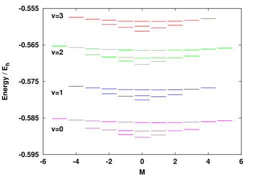
Figure 9: Rotational structure, up to $L=5$, of the four lowest vibrational states of $\rm H_{2}^{+}$ in the presence of an external magnetic field of $B=0.2B_{0}$. All states are located above the rotational barrier, which is at $E=-0.595678\;E_{h}$.

5 Conclusions

We have investigated the problem of $\rm H_{2}^{+}$ and $\rm D_{2}^{+}$ in an external magnetic field of up to $B=0.2B_{0}$ or 4.7$\times 10^{4}$ T by exact and approximate methods. This includes a thorough analysis of the electronic energy as function of field strength and orientation of the molecule with respect to the external field as well as of the rovibrational structure of $\rm H_{2}^{+}$ and $\rm D_{2}^{+}$. The electronic problem has been solved by the variational method with physically adequate trial functions. It is shown that both diamagnetic and paramagnetic susceptibilities grow with inclination, while paramagnetic susceptibility is systematically much smaller than the diamagnetic one. Evaluation of the magnetic susceptibility shows that first-order perturbation theory based on zero-field trial functions may no longer be accurate at a field strength of above $B\approx 0.04B_{0}$. To solve the ro-vibrational problem, the hindered rotor approximation, in which the potential energy surface is approximated by a zero-inclination potential curve as a function of the internuclear distance $R$ and a simple parametrization of the rotational barrier in the angular coordinate $\theta$ gives results accurate to about $10^{-5}\;E_{h}$, which is comparable in accuracy with the rigid-rotor approximation to separate vibrational and rotational motion. Some of the approximations have been used before, by other authors, at much higher field strengths, were they are less accurate. The findings of the present paper provide a basis for future investigations dealing with higher field strengths and different molecules such as $\rm H_{2}$.

Acknowledgements

H.M.C. is grateful to Consejo Nacional de Ciencia y Tecnología, Mexico, for a postdoctoral grant (CONACyT grant no 202139). This work was also supported by a Mexican-French binational research grant (CONACyT-CNRS grant no 26218) and by the Computer Center ROMEO of the University of Reims Champagne-Ardenne. Research by J.C.L.V and A.V. T. was supported in part by CONACyT grant 116189 and DGAPA IN109512.

References

- [1] C. P. de Melo, R. Ferreira, H. S. Brandi and L. C. M. Miranda, Phys. Rev. Lett. 37 676 (1976).
- [2] U. Kappes and P. Schmelcher, Phys. Rev. A 51 4542 (1995).
- [3] A. V. Turbiner, Usp. Fiz. Nauk. 144 35 (1984). A. V. Turbiner, Sov. Phys. –Uspekhi 27 668 (1984) (Engl. Trans.)
- [4] A. V. Turbiner, Yad. Fiz. 46 204 (1987). A. V. Turbiner, Sov. J. Nucl. Phys 46 125 (1987) (Engl. Trans.)
- [5] A. V. Turbiner and J. C. López Vieyra, Phys. Rev. A 68 012504 (2003).
- [6] A. V. Turbiner and J. C. López Vieyra, Phys. Rev. A 69 053413 (2004).
- [7] A. V. Turbiner and J. C. López Vieyra, Phys. Rep. 242 309 (2006).
- [8] D. M. Larsen, Phys. Rev. A 76 042502 (2007).
- [9] D. Baye, A. Joos de ter Beerst and J-M Sparenberg, J. Phys. B: At. Mol. Opt. Phys. 42 225102 (2009).
- [10] X. Song, C. Gong, X. Wang and H. Qiao, J. Chem. Phys. 139 064305 (2013).
- [11] J. Avron, I. Herbst and B. Simon, Ann. Phys. 114, 431 (1978).
- [12] P. Schmelcher and L. S. Cederbaum, Phys. Rev. A 37, 672 (1988).
- [13] P. Schmelcher, L. S. Cederbaum and H.-D. Meyer, Phys. Rev. A 38, 6066 (1988).
- [14] A. V. Turbiner Astrophys. Space Sci. 308 267-277 (2007).
- [15] A. V. Turbiner, N. L. Guevara and J. C. López Vieyra, Phys. Rev. 75 053408 (2007).
- [16] A. V. Turbiner, J. C. López Vieyra and N. L. Guevara, Phys. Rev. A 81 042503 (2010).
- [17] D. M. Larsen, Phys. Rev. A 25 1295 (1982).
- [18] U. Wille, J. Phys. B: At. Mol. Phys. 20 L417 (1987).
- [19] D. H. Kobe and P. K. Kennedy, J. Chem. Phys. 80, 3710 (1983).
- [20] A. Y. Potekhin and A. V. Turbiner, Phys. Rev. A 63, 065402 (2001).
- [21] L. D. Landau, and E. M. Lifshitz, Quantum Mechanics. Non-Relativistic Theory, pag. 463-470, Butterworth-Heinemann (2003).
- [22] L. D. Landau, and E. M. Lifshitz, Statistical Physics: Part 1, pag. 152-157, Pergamon Press Ltd. (1980).
- [23] T. K. Rebane Optics and Spectroscopy, 93, pp. 236-241 (2002)
- [24] D. Zeroka and T. B. Garrett, J. Am. Chem. Soc. 90, 6282 (1968).
- [25] T. B. Garrett and D. Zeroka, Intern. J. Quantum Chem. 6, 651 (1972).
- [26] R. A. Hegstrom, Phys. Rev. A 19, 17 (1979).
- [27] V. Magnasco, Elementary Methods of Molecular Quantum Mechanics, pag. 456-457, Elsevier, Amsterdam (2007).