Phase separation in a spin-orbit coupled Bose-Einstein condensate

Abstract

We study a spin-orbit (SO) coupled hyperfine spin-$1$ Bose-Einstein condensate (BEC) in a quasi-one-dimensional trap. For a SO-coupled BEC in a one-dimensional box, we show that in the absence of the Rabi term, any non-zero value of SO coupling will result in a phase separation among the components for a ferromagnetic BEC, like ⁸⁷Rb. On the other hand, SO coupling favors miscibility in a polar BEC, like ²³Na. In the presence of a harmonic trap, which favors miscibility, a ferromagnetic BEC phase separates, provided the SO-coupling strength and number of atoms are greater than some critical value. The Rabi term favors miscibility irrespective of the nature of the spin interaction: ferromagnetic or polar.

I Introduction

A Bose-Einstein condensate (BEC) with spin degrees of freedom, known as a spinor BEC, was first experimentally realized and studied in a gas of ²³Na atoms, with hyperfine spin $F=1$, in an optical dipole trap Stamper-Kurn . This has lead to a flurry of investigation on both the theoretical and experimental fronts, which has been reviewed in Ref. ueda . In the present work, we study the ground state structure of the $F=1$ spin-orbit (SO) coupled spinor BEC in a quasi-one-dimensional (quasi-1D) trap luca within the framework of the mean-field theory. The mean-field theory to study $F=1$ spinor BECs was developed independently by Ohmi et al. Ohmi and Ho Ho . The SO-interaction is absent in neutral atoms and an engineering with an external electromagnetic field is needed for its experimental realization. A variety of SO couplings can be engineered by counter propagating Raman lasers coupling the hyperfine states, and the parameters of this coupling can be controlled independently young . The SO interaction has been achieved recently with equal strengths of Rashba Bychkov and Dresselhaus Dresselhaus ; Liu couplings employing a necessary engineering to obtain experimentally a SO-coupled BEC of two of the existing three hyperfine spin components of the $F=1$ state of ⁸⁷Rb Lin ; Linx forming a pseudo-spinor BEC. This has been followed by other experiments on SO-coupled pseudo-spinor BECs JY_Zhang . In the case of a $F=1$ spinor BEC, there are theoretical proposals to realize SO-coupling interaction involving the three hyperfine spin components Juzeliunas . SO-coupled degenerate Fermi gases (⁴⁰K and ⁶Li) have also been experimentally realized P_Wang . A mean-field Gross-Pitaevskii (GP) equation for the theoretical study of dynamics in SO-coupled BECs has also been proposed Juzeliunas ; ueda ; H_Wang ; Bao .

The ground states of the SO-coupled two-component pseudo- spinor BEC and of the three-component spinor BEC have been theoretically investigated by Wang et al. Wang . It has further been established that the SO-coupled spin-$1/2$ (pseudo-spinor), $F=1$ and $F=2$ spinor BECs in quasi-two-dimensional (quasi-2D) traps luca can have a variety of nontrivial ground state structures Gopalakrishnan ; Xu-1 ; Ruokokoski . There have been studies of intrinsic spin-Hall effect Larson , chiral confinement Merkl , superfluidity super , Josephson oscillation josep , vortices vor , and solitons sol in a SO-coupled BECs. In general, for experimentally feasible parameters, the ground state of a $F=1$ spinor BEC can host a single vortex or a square vortex lattice for weak and strong SO coupling, respectively Ruokokoski . Additionally, plane and standing wave states appear as ground states in the case of ferromagnetic and polar (antiferromagnetic) BECs, respectively, for medium strengths of SO coupling Ruokokoski . The ground state of the $F=1$ spinor BEC in the presence of a homogeneous magnetic field has also been studied  Zhou ; Matuszewski-1 ; Matuszewski-2 . It was shown in Refs. Matuszewski-1 ; Matuszewski-2 that a uniform magnetic field can lead to a phase separation in polar BEC. Phase separation has already been observed in a pseudo-spinor BEC consisting of two hyperfine states of ⁸⁷Rb in quasi-2D geometries Lin .

In this paper, we investigate the ground state of a SO-coupled $F=1$ spinor BEC in a quasi-1D trap. For the model of SO-coupling employed in this work, we find that compared to the homogeneous magnetic field, SO coupling leads to a phase separation in the case of a ferromagnetic BEC, whereas in the case of a polar BEC, it makes the miscible profile energetically more stable. Here, we use a numerical solution of the generalized mean-field GP equation H_Wang ; Bao to study the possible phase separation between the different hyperfine spin components of a SO-coupled BEC. We also study the possibility of a phase separation in a uniform spinor condensate in a 1D box employing an analytical model. The results of this analytical study provide a qualitative understanding of the numerical findings for a trapped SO-coupled BEC.

The paper is organized as follows. In Sec. II, we describe the coupled GP equation used to study the SO-coupled $F=1$ spinor BEC in a quasi-1D trap. This is followed by an analytical investigation of a SO-coupled spinor BEC in a 1D box in Sec. III. By comparing the energies of various competing geometries for both ferromagnetic and polar BECs, the ground state structure is determined from a minimization of energy. In the case of a mixture of two scalar BECs, similar analysis leads to the criterion for a phase separation Ao . In Sec. IV, we numerically study the SO-coupled spinor BEC in a quasi-1D trap. We conclude the manuscript by providing a summary of this study in Sec. V.

II Mean-field model for a SO-coupled BEC

For the electronic states of a hydrogen-like atom the SO contribution to the atomic spectrum naturally appears because of the magnetic energy of this coupling existing due to electronic charge. In the case of the hyperfine states of neutral atoms, an engineering with external electromagnetic fields is required for the SO coupling to contribute to the BEC. We use the SO-coupled interaction of the experiment of Lin et al. Lin for two hyperspin components of the ⁸⁷Rb hyperfine state 5S_1/2, realized with strength $\gamma$ using two counterpropagating Raman lasers of wavelength $\lambda_{r}$ oriented at an angle $\beta_{r}$: $\gamma=\hbar k_{r}/m$, where $k_{r}=2\pi\sin(\beta_{r}/2)/\lambda_{r}$ and $m$ is the mass of an atom. This SO coupling is equivalent to that of an electronic system with equal contribution of Rashba Bychkov and Dresselhaus Dresselhaus couplings and with an external uniform magnetic field. However, here we consider the SO coupling among the three spin components of the $F=1$ state, e.g., $|F=1,m_{F}=1\rangle$, $|F=1,m_{F}=0\rangle$, and $|F=1,m_{F}=-1\rangle$, where $m_{F}$ is the $z$ projection of $F$. It has been shown lan that this SO coupling among the three hyperfine spin components can be generated by an engineering as in Ref. Lin . We will consider the three spin components of the $F=1$ hyperfine state 5S_1/2 of ⁸⁷Rb and 3S_1/2 of ²³Na.

We consider such a quasi-1D hyperfine spin-$1$ SO-coupled spinor BEC confined along the $x$-axis obtained by making the trap along $y$ and $z$ axes much stronger than that along the $x$-axis. The transverse dynamics of the BEC is assumed to be frozen to the respective ground states of harmonic traps. Then, the single-particle quasi-1D Hamiltonian of the system under the action of a strong transverse trap of angular frequencies $\omega_{y}$ and $\omega_{z}$ along $y$ and $z$ directions respectively, can be written as Lin ; Y_Zhang

$$H_{0}=\frac{p_{x}^{2}}{2m}+\gamma p_{x}\Sigma_{z}+\Omega\Sigma_{x},$$ (1)

where $p_{x}=-i\hbar\partial_{x}$ is the momentum operator along $x$ axis, $\Omega$ is the Rabi frequency Lin ; Linx , and $\Sigma_{z}$ and $\Sigma_{x}$ are the matrix representations of the $z$ and $x$ components of the spin-1 angular momentum operator, respectively, and are given by

$$\Sigma_{z}=\left(\begin{array}[]{ccc}1&0&0\\ 0&0&0\\ 0&0&-1\end{array}\right),\quad\Sigma_{x}=\frac{1}{\sqrt{2}}\left(\begin{array}[]{ccc}0&1&0\\ 1&0&1\\ 0&1&0\end{array}\right).$$ (8)

If the interactions among the atoms in the BEC are taken into account, in the Hartree approximation, using the single particle model Hamiltonian (1), a quasi-1D luca spinor BEC can be described by the following set of three coupled mean-field partial differential GP equations for the wave-function components $\psi_{j}$ H_Wang ; Bao ; ueda

$$i\hbar\frac{\partial\psi_{1}}{\partial t} = \left(-\frac{\hbar^{2}}{2m}\frac{\partial^{2}}{\partial x^{2}}+V(x)+c_{0}\rho\right)\psi_{1}+c_{2}(\rho_{1}+\rho_{0}-$$ (9)

$$\rho_{-1})\psi_{1}+c_{2}\psi_{-1}^{*}\psi_{0}^{2}-i\hbar\gamma\frac{\partial\psi_{1}}{\partial x}+\frac{\Omega}{\sqrt{2}}\psi_{0},$$

$$i\hbar\frac{\partial\psi_{0}}{\partial t} = \left(-\frac{\hbar^{2}}{2m}\frac{\partial^{2}}{\partial x^{2}}+V(x)+c_{0}\rho\right)\psi_{0}+c_{2}(\rho_{1}+\rho_{-1})$$ (10)

$$\psi_{0}+2c_{2}\psi_{1}\psi_{-1}\psi_{0}^{*}+\frac{\Omega}{\sqrt{2}}(\psi_{1}+\psi_{-1}),$$

$$i\hbar\frac{\partial\psi_{-1}}{\partial t} = \left(-\frac{\hbar^{2}}{2m}\frac{\partial^{2}}{\partial x^{2}}+V(x)+c_{0}\rho\right)\psi_{-1}+c_{2}(\rho_{0}+\rho_{-1}$$ (11)

$$-\rho_{1})\psi_{-1}+c_{2}\psi_{1}^{*}\psi_{0}^{2}+i\hbar\gamma\frac{\partial\psi_{-1}}{\partial x}+\frac{\Omega}{\sqrt{2}}\psi_{0},$$

where $V(x)=m\omega_{x}^{2}x^{2}/2$ is the 1D harmonic trap, $c_{0}=2\hbar^{2}(a_{0}+2a_{2})/(3ml_{yz}^{2})$, $c_{2}=2\hbar^{2}(a_{2}-a_{0})/(3ml_{yz}^{2})$, $a_{0}$ and $a_{2}$ are the $s$-wave scattering lengths in the total spin $0$ and $2$ channels, respectively, $\rho_{j}=|\psi_{j}|^{2}$ with $j=1,0,-1$ are the component densities, $\rho=\sum_{j=-1}^{1}|\psi_{j}|^{2}$ is the total density, and $l_{yz}=\sqrt{\hbar/(m\omega_{yz})}$ with $\omega_{yz}=\sqrt{\omega_{y}\omega_{z}}$ is the oscillator length in the transverse $y-z$ plane. The normalization condition is

$$\int_{-\infty}^{\infty}dx\sum_{j=-1}^{1}|\psi_{j}(x)|^{2}=N.$$ (12)

In order to transform Eqs. (9) - (11) into dimensionless form, we use the scaled variables defined as

$$\tilde{t}=\omega_{x}t,~{}\tilde{x}=\frac{x}{l_{0}},~{}\phi_{j}(\tilde{x},\tilde{t})=\frac{\sqrt{l_{0}}}{\sqrt{N}}\psi_{j}(\tilde{x},\tilde{t}),$$ (13)

where $l_{0}=\sqrt{\hbar/(m\omega_{x}}$) is the oscillator length along $x$-axis, $N$ is the total number of the atoms. Using these dimensionless variables, the coupled mean-field Eqs. (9) - (11) in dimensionless form are

$$i\frac{\partial\phi_{1}}{\partial\tilde{t}} = \left(-\frac{1}{2}\frac{\partial^{2}}{\partial\tilde{x}^{2}}+\tilde{V}+\tilde{c}_{0}\tilde{\rho}\right)\phi_{1}+\tilde{c}_{2}(\tilde{\rho}_{1}+\tilde{\rho}_{0}$$ (14)

$$-\tilde{\rho}_{-1})\phi_{1}+\tilde{c}_{2}\phi_{-1}^{*}\phi_{0}^{2}-i\tilde{\gamma}\frac{\partial\phi_{1}}{\partial\tilde{x}}+\frac{\tilde{\Omega}}{\sqrt{2}}\phi_{0},$$

$$i\frac{\partial\phi_{0}}{\partial\tilde{t}} = \left(-\frac{1}{2}\frac{\partial^{2}}{\partial\tilde{x}^{2}}+\tilde{V}+\tilde{c}_{0}\tilde{\rho}\right)\phi_{0}+\tilde{c}_{2}(\tilde{\rho}_{1}+\tilde{\rho}_{-1})$$ (15)

$$\phi_{0}+2\tilde{c}_{2}\phi_{1}\phi_{-1}\phi_{0}^{*}+\frac{\tilde{\Omega}}{\sqrt{2}}(\phi_{1}+\phi_{-1}),$$

$$i\frac{\partial\phi_{-1}}{\partial\tilde{t}} = \left(-\frac{1}{2}\frac{\partial^{2}}{\partial\tilde{x}^{2}}+\tilde{V}+\tilde{c}_{0}\tilde{\rho}\right)\phi_{-1}+\tilde{c}_{2}(\tilde{\rho}_{0}+\tilde{\rho}_{-1}$$ (16)

$$-\tilde{\rho}_{1})\phi_{-1}+\tilde{c}_{2}\phi_{1}^{*}\phi_{0}^{2}+i\tilde{\gamma}\frac{\partial\phi_{-1}}{\partial\tilde{x}}+\frac{\tilde{\Omega}}{\sqrt{2}}\phi_{0},$$

where $\tilde{V}=\tilde{x}^{2}/2$, $\tilde{\gamma}=\hbar k_{r}/(m\omega_{x}l_{0})$, $\tilde{\Omega}=\Omega/(\hbar\omega_{x})$, $\tilde{c}_{0}=2N(a_{0}+2a_{2})/(3l^{2}_{yz})$, $\tilde{c}_{2}=2N(a_{2}-a_{0})/(3l^{2}_{yz})$, $\tilde{\rho}_{j}=|\phi_{j}|^{2}$ with $j=1,0,-1$, and $\tilde{\rho}=\sum_{j=-1}^{1}|\phi_{j}|^{2}$. The normalization condition satisfied by $\phi_{j}$’s is

$$\int_{-\infty}^{\infty}\sum_{j=-1}^{1}\tilde{\rho}_{j}(\tilde{x})d\tilde{x}=1.$$ (17)

Another useful quantity $-$ magnetization $-$ related to the component densities is defined by

$${\cal M}=\int_{-\infty}^{\infty}[\tilde{\rho}_{1}(\tilde{x})-\tilde{\rho}_{-1}(\tilde{x})]d\tilde{x}.$$ (18)

Depending on the value of $\tilde{c}_{2}$ ($>0$ or $<0$) the system develops interesting physical properties. The interaction in the $5$S_1/2 state of ⁸⁷Rb with $\tilde{c}_{2}<0$ is termed ferromagnetic and that in the $3$S_1/2 state of ²³Na with $\tilde{c}_{2}>0$ is termed antiferromagnetic or polar. For the sake of simplicity of notations, we will represent the dimensionless variables without tilde in the rest of the paper.

The energy of the spinor BEC in the presence of a SO coupling is Bao ; H_Wang

$$E = N\int_{-\infty}^{\infty}\Bigg{\{}\frac{1}{2}\left|\frac{d\phi_{1}}{dx}\right|^{2}+\frac{1}{2}\left|\frac{d\phi_{0}}{dx}\right|^{2}+\frac{1}{2}\left|\frac{d\phi_{-1}}{dx}\right|^{2}+V\rho$$ (19)

$$+\frac{c_{0}}{2}\rho^{2}+\frac{c_{2}}{2}\left(\rho_{1}+\rho_{0}-\rho_{-1}\right)\rho_{1}+\frac{c_{2}}{2}\left(\rho_{1}+\rho_{-1}\right)\rho_{0}$$

$$+\frac{c_{2}}{2}\left(\rho_{0}+\rho_{-1}-\rho_{1}\right)\rho_{-1}+c_{2}\left[\phi_{-1}^{*}\phi_{0}^{2}\phi_{1}^{*}\right.$$

$$\left.+\phi_{-1}(\phi_{0}^{*})^{2}\phi_{1}\right]+\gamma\left(-i\phi_{1}^{*}\frac{d\phi_{1}}{dx}+i\phi_{-1}^{*}\frac{d\phi_{-1}}{dx}\right)$$

$$+\frac{\Omega}{\sqrt{2}}\left(\phi_{1}^{*}\phi_{0}+\phi_{0}^{*}\phi_{1}+\phi_{-1}^{*}\phi_{0}+\phi_{0}^{*}\phi_{-1}\right)\Bigg{\}}dx.$$

Based on the form of this energy functional a few inferences can be easily drawn about the phase separation among the various components of a spinor BEC with SO coupling. The energy term proportional to $c_{0}$ can never lead to a phase separation as it contains terms $Nc_{0}\int(\rho_{j}^{2}/2+\rho_{j}\rho_{j^{\prime}})dx$, where $j,j^{\prime}=1,0,-1$ and $j\neq j^{\prime}$, and hence corresponds to a scenario where inter- and intra-species interactions are of equal strengths. The situation is analogous to a binary BEC with $a_{12}^{2}=a_{11}a_{22}$, where $a_{11}$ and $a_{22}$ are intra-species and $a_{12}$ the inter-species scattering lengths. Such a binary BEC has equal strengths of inter- and intra-species nonlinearities and is always miscible in the presence of a $1$D harmonic trap Ao ; Gautam . Let us now look at the terms proportional to $c_{2}$. For the stable solution, the phases of the three components, say $\theta_{j}$’s with $j=-1,0,1$, should satisfy

$$\theta_{1}+\theta_{-1}+s\pi=2\theta_{0},$$ (20)

where $s$ is an integer Matuszewski-2 ; Isoshima . Assuming that $\theta_{0}=0$ and $s=0$, the interaction energy part of the total energy (19) can be written as

$$E_{\rm int} =N\int_{-\infty}^{\infty}\biggr{\{}\frac{c_{0}}{2}\rho^{2}+\frac{c_{2}}{2}\left(\rho_{1}^{2}+\rho_{-1}^{2}+2\rho_{1}\rho_{0}+2\rho_{0}\rho_{-1}\right.$$

$$\left.-2\rho_{1}\rho_{-1}+4\sqrt{\rho_{1}\rho_{-1}}\rho_{0}\right)\biggr{\}}dx.$$ (21)

The system will naturally move to a state of minimum energy, which could have a phase-separated or an overlapping configuration. A consideration of minimization of energy could reveal whether the system will prefer a ground state with an overlapping or a phase-separated profile.

It is evident from Eq. (II) that in the case of a ferromagnetic BEC ($c_{2}<0$), there is only one term $N\int|c_{2}|\rho_{1}\rho_{-1}dx$ with positive energy contribution representing inter-species repulsion, which will favor a phase separation between components $1$ and $-1$. The minimum contribution from this term can be zero, when components $1$ and $-1$ are fully phase-separated, whereas, for the rest of the $c_{2}$ dependent terms in $E_{\rm int}$, the contribution is always less than zero representing inter-species attraction. A maximum of overlap between the components will reduce the contribution of these terms to energy. Hence these terms will inhibit a phase separation. So, the phase separation in a ferromagnetic BEC, if ever it occurs, can only take place between components $1$ and $-1$.

On the other hand in the case of a polar or antiferromagnetic BEC ($c_{2}>0$), all the terms in Eq. (II) except $-N\int c_{2}\rho_{1}\rho_{-1}dx$ contribute positive energy representing inter-species repulsion. For an arbitrary value of magnetization $\cal{M}$, the interaction energy can be minimized in two ways. First, by making $\rho_{0}=0$ and ensuring the maximum overlap between components $1$ and $-1$; and, secondly, by fully phase-separating the $0$th component from the maximally overlapping $1$ and $-1$ components. The interaction energy in both the cases becomes

$$E_{\rm int}=N\int_{-\infty}^{\infty}\Bigg{\{}\frac{c_{0}}{2}\rho^{2}+\frac{c_{2}}{2}\left(\rho_{1}^{2}+\rho_{-1}^{2}-2\rho_{1}\rho_{-1}\right)\Bigg{\}}dx.$$ (22)

Hence, the phase separation in a polar BEC, if it ever occurs, is most likely to take place between the $0$th component and overlapping $1$ and $-1$ components.

III SO-coupled BEC in a 1D box

To understand the role of the different terms in the expression for the interaction energy (II) on phase separation, we study an analytic model of a uniform (trapless) spinor BEC in a 1D box of length $2L$ localized in the region $-L<x<L$. In order to clearly establish the role of the different terms in $E_{\rm int}$ in determining the ground state structure of the $F=1$ spinor BEC, first we consider the one with zero magnetization ($\cal M=$ 0).

We consider the miscible and immiscible profiles in the case of a ferromagnetic BEC ($c_{2}<0$). In the miscible case, the densities are uniform and written as $\rho_{j}(x)\equiv n_{j}$. Because of the symmetry between $j=1$ and $j=-1$, it is natural to take $n_{1}=n_{-1}$. Then the densities of the three components can be written as

$$\rho_{1}(x) = n_{1},\quad\quad\quad\quad-L<x<L,$$ (23)

$$\rho_{0}(x) = n_{0},\quad\quad\quad\quad-L<x<L,$$ (24)

$$\rho_{-1}(x) = n_{-1}=n_{1},\quad-L<x<L.$$ (25)

All densities are zero for $|x|\geq L$. This is the general density distribution for a miscible configuration which we will use in this study. In the absence of a SO coupling and Rabi term $(\gamma=\Omega=0)$, the interaction energy (II) for a ferromagnetic BEC in the 1D box becomes

$$E_{\rm int} = NL[c_{0}(4n_{1}^{2}+n_{0}^{2}+4n_{1}n_{0})-|c_{2}|8n_{1}n_{0}],$$ (26)

and the corresponding normalization condition is

$$2L(2n_{1}+n_{0})=1.$$ (27)

In the trapped case, as considered in Sec. II, the energies (19) or (II) are extensive properties and increase with the size of the system. However, the energy density (energy per unit length) of a uniform gas, as considered in this section, is an intensive property Ao and does not depend on system size or the total length of the box, provided that a constant particle density is maintained when the size is changed. Recalling that the constants $c_{0}$ and $c_{2}$ are proportional to the number of atoms $N$, Eq. (26), and all other energies in this section reveal the interesting feature

$$\frac{E_{\rm int}}{L}\sim\left(\frac{N}{L}\right)^{2},$$ (28)

also valid for nonspinor systems Ao . The minimum of energy (26), subject to the normalization constraint (27) and for $n_{j}$’s $\geq 0$, occurs at

$$n_{1}=n_{-1}^{\prime}=\frac{1}{8L},~{}n_{0}=\frac{1}{4L},$$ (29)

and the corresponding minimum energy is

$$E_{\rm int}^{\rm min(M)}=N\frac{(c_{0}-|c_{2}|)}{4L}.$$ (30)

In the immiscible case, where components $j=1$ and $j=-1$ are separated, let $n_{1}^{\prime}$ be the density of component $1$ from $-L$ to $0$ and $n_{-1}^{\prime}=n_{1}^{\prime}$ be the density of component $-1$ from $0$ to $L$. This symmetric distribution is consistent with the symmetry between components $j=1$ and $-1$ in the mean-field Eqs. (14)-(16). The density of component $0$ distributed from $-L$ to $L$ is taken to be $n_{0}^{\prime}$ as in the miscible case, so that,

$$\rho_{1}(x) = \left\{\begin{array}[]{lr}n_{1}^{\prime},&\quad\quad\quad\quad-L<x<0,\\ 0,&\quad\quad\quad\quad~{}0\leq x\leq L,\end{array}\right.$$ (33)

$$\rho_{0}(x) = \begin{array}[]{lr}n_{0}^{\prime},&\quad\quad\quad\quad\quad-L<x<L,\\ \end{array}$$ (35)

$$\rho_{-1}(x) = \left\{\begin{array}[]{lr}n_{-1}^{\prime}=n_{1}^{\prime},&~{}0<x<L,\\ 0,&~{}-L\leq x\leq 0.\end{array}\right.$$ (38)

All densities are zero for $|x|\geq L$. This is the general density distribution for an immiscible configuration, which we will use in this study for the ferromagnetic condensate. As mentioned in Sec. II, for a ferromagnetic BEC, a phase separation between the $1$ and $-1$ components is energetically the most favorable among all other possible phase separations. This is the reason to choose the aforementioned distribution for the immiscible profile. The interaction energy for this distribution is

$$E_{\rm int}=NL[c_{0}(n_{1}^{\prime 2}+n_{0}^{\prime 2}+2n_{1}^{\prime}n_{0}^{\prime})-|c_{2}|n_{1}^{\prime}(n_{1}^{\prime}+2n_{0}^{\prime})],$$ (39)

with the normalization condition

$$2L(n_{1}^{\prime}+n_{0}^{\prime})=1.$$ (40)

The condition of the minimum of energy in this case, again subject to the normalization constraint  (40) and for $n_{j}$’s $\geq 0$, is

$$n_{1}^{\prime}=n_{-1}^{\prime}=\frac{1}{2L},~{}n_{0}^{\prime}=0,$$ (41)

and the minimum value of interaction energy $E_{\rm int}^{\rm min(I)}$ is the same as in the miscible case, given by Eq. (30): $E_{\rm int}^{\rm min(M)}=E_{\rm int}^{\rm min(I)}$. Thus, from an energetic consideration, the miscible and immiscible profiles are equally favorable in a homogeneous ferromagnetic BEC in the absence of a confining trap. Now, $n_{1}^{\prime}=n_{-1}^{\prime}=1/(2L)$ are the maximum density values allowed for these two components of the system with zero magnetization for the immiscible case. Any general distribution with zero magnetization for the immiscible profile will have, due to the inherent symmetry of the present model between components $j=1$ and -1, $n_{1}^{\prime}=1/(2L)-\delta$ between $x=-L$ to $0$, $n_{-1}^{\prime}=1/(2L)-\delta$ between $x=0$ to $L$, and $n_{0}^{\prime}=\delta$ between $x=-L$ to $L$, with $\delta\geq 0$. The interaction energy corresponding to this general distribution for the immiscible profile is

$$E_{\rm int}=N\left[\frac{c_{0}-|c_{2}|}{4L}+|c_{2}|\delta^{2}L\right].$$ (42)

Hence, the interaction energy for this immiscible profile is either more than $(\delta>0)$ or equal to $(\delta=0)$ the interaction energy of the miscible one. Hence for a general distribution ($\delta\neq 0$) the miscible profile with the lowest energy will be the preferred ground state. The presence of a trapping potential, however small it may be, will favor the miscible profile due to an extra confining force to the center.

Now let us consider the phase separation in a polar BEC. Interaction energy (II) can be minimized if we choose

$$n_{1}=n_{-1}=\frac{1}{4L},n_{0}=0$$ (43)

in the case of a miscible profile [viz. Eqs. (23)-(25)] or $n_{1}=n_{-1}=0,n_{0}=1/(2L)$ in the case of an immiscible profile [viz. Eqs. (33)-(38)]. This immiscible profile represents effectively a single component system. The value of the minimum energy in both the cases is

$$E_{\rm int}^{\rm min}=\frac{Nc_{0}}{4L}.$$ (44)

As mentioned in Sec. II, the phase-separation in polar condensate is most likely to occur between the $0$th and overlapping $1$ and $-1$ components. Therefore, we also consider the profile where the components $1$ and $-1$ are miscible, and these two are phase separated from the $0$th component with the following general density distribution

$$\rho_{1}(x) = \left\{\begin{array}[]{lr}n_{1}^{\prime\prime},&\quad\quad\quad\quad-L<x<-L+L^{\prime},\\ 0,&\quad\quad\quad\quad~{}-L+L^{\prime}\leq x\leq L,\end{array}\right.$$ (47)

$$\rho_{0}(x) = \left\{\begin{array}[]{lr}0,&\quad\quad\quad\quad~{}-L<x<-L+L^{\prime},\\ n_{0}^{\prime\prime},&\quad\quad\quad\quad\quad-L+L^{\prime}\leq x\leq L,\end{array}\right.$$ (50)

$$\rho_{-1}(x) = \left\{\begin{array}[]{lr}n_{-1}^{\prime\prime}=n_{1}^{\prime\prime},&~{}-L<x<-L+L^{\prime},\\ 0,&~{}-L+L^{\prime}\leq x\leq L,\end{array}\right.$$ (53)

where $L^{\prime}<2L$, and all the densities are zero for $|x|>L$. The interaction energy for this distribution is

$$E_{\rm int}=\frac{Nc_{0}}{2}[4(n_{1}^{\prime\prime})^{2}L^{\prime}+2(n_{0}^{\prime\prime})^{2}L-(n_{0}^{\prime\prime})^{2}L^{\prime}],$$ (54)

with the normalization condition

$$2n_{1}^{\prime\prime}L^{\prime}+2n_{0}L-n_{0}L^{\prime}=1.$$ (55)

The minimum of this energy, subject to the normalization constraint, occurs at

$$L^{\prime}=L,~{}n_{1}^{\prime\prime}=n_{-1}^{\prime\prime}=\frac{1}{4L},~{}\rm{and}~{}n_{0}^{\prime\prime}=\frac{1}{2L}.$$ (56)

The minimum interaction energy for this density distribution is the same as for the miscible profile, i.e., $E_{\rm int}^{\rm min}=Nc_{0}/(4L)$. Similarly, it can be shown that the profile where all the three components are phase separated from each other as well as the rest of the possible phase separated profiles, the interaction energy is always greater than $Nc_{0}/(4L)$ due to a non-zero contribution from the $c_{2}$ dependent terms. So, the energy of any general immiscible profile is either equal to or greater than $Nc_{0}/(4L)$ due to a non-zero contribution from the $c_{2}$ dependent terms. The presence of a trapping potential, however weak it may be, will make the miscible profile energetically more favorable than the all possible immiscible profiles. Hence, there can be no phase separation in the trapped ferromagnetic and polar BECs.

Next let us consider the effect of the SO coupling and the Rabi term on a phase separation. First, let us include the SO coupling without the Rabi term $(\gamma\neq 0,\Omega=0)$ and discuss the effect on a ferromagnetic BEC $(c_{2}<0)$. The presence of this term leads to a constant phase gradient $-\alpha$ and $\alpha$ in $\phi_{1}$ and $\phi_{-1}$, respectively Bao . The interaction energy of the miscible profile [viz. Eqs. (23)-(25)] in this case is

$$E_{\mathrm{int}} = NL\left[c_{0}(4n_{1}^{2}+n_{0}^{2}+4n_{1}n_{0})-|c_{2}|8n_{1}n_{0}\right.$$ (57)

$$\left.+2\alpha^{2}n_{1}-4\gamma\alpha n_{1}\right],$$

where the $2N\alpha^{2}n_{1}L$ term arises from the derivatives of the phases of $\phi_{1}$ and $\phi_{-1}$. Minimizing this energy with respect to $n_{1}$ and $\alpha$, subject to the normalization constraint  (27) and $n_{j}\geq 0$ for $j=1,0,-1$, we get

$$\alpha=\gamma,~{}n_{1}=\left\{\begin{array}[]{lr}\frac{1}{8L}+\frac{\gamma^{2}}{16|c_{2}|},&\gamma\leq\sqrt{2|c_{2}|/L}\\ \frac{1}{4L},&\gamma>\sqrt{2|c_{2}|/L},\end{array}\right.$$ (58)

with the corresponding minimum energy

$$E^{\rm min(M)}_{\mathrm{int}}=\left\{\begin{array}[]{lr}N\left[\frac{c_{0}-|c_{2}|}{4L}-\frac{\gamma^{2}}{4}-\frac{L\gamma^{4}}{16|c_{2}|}\right],&\gamma\leq\sqrt{2|c_{2}|/L}\\ N\left[\frac{c_{0}}{4l}-\frac{\gamma^{2}}{2}\right],&\gamma>\sqrt{2|c_{2}|/L}.\end{array}\right.$$ (61)

The density $n_{1}$ of Eq. (58) attains a saturation for $\gamma>\sqrt{2|c_{2}|/L}$. With further increase of $\gamma$ the density $n_{1}$ does not change as it has already achieved the maximum permissible density for a state with ${\cal M}=0$ subject to the normalization constraint  (27).

The interaction energy of the immiscible profile [viz. Eqs. (33)-(38)] in this case is

$$E_{\mathrm{int}} = NL[c_{0}(n_{1}^{\prime 2}+n_{0}^{\prime 2}+2n_{1}^{\prime}n_{0}^{\prime})-|c_{2}|n_{1}^{\prime}(n_{1}^{\prime}+2n_{0}^{\prime})$$ (62)

$$+\alpha^{\prime 2}n_{1}^{\prime}-2\gamma\alpha^{\prime}n_{1}^{\prime}],$$

Minimizing this energy with respect to $n_{1}^{\prime}$ and $\alpha^{\prime}$, subject to the normalization constraint  (40) and $n_{j}\geq 0$ for $j=1,0,-1$, we get

$$\alpha^{\prime}=\gamma,~{}n_{1}^{\prime}=\frac{1}{2L},$$ (63)

with the corresponding minimum energy

$$E^{\rm min(I)}_{\mathrm{int}}=N\left[\frac{c_{0}-|c_{2}|}{4L}-\frac{\gamma^{2}}{2}\right].$$ (64)

Comparing Eqs. (61) and (64), we find that the immiscible profile has lower energy than the miscible one for any non-zero value of $\gamma$ for a ferromagnetic BEC: $E_{\rm{int}(\Omega)}^{\rm min(I)}<E_{\rm{int}(\Omega)}^{\rm min(M)}$. Hence the SO coupling will favor phase separation in a ferromagnetic BEC.

Let us now discuss the phase separation in a polar BEC in the presence of a SO coupling. The interaction energy of the miscible profile [viz. Eqs. (23)-(25)] in this case is

$$E_{\rm{int}} = NL[c_{0}(4n_{1}^{2}+n_{0}^{2}+4n_{1}n_{0})+8c_{2}n_{1}n_{0}$$ (65)

$$+2\alpha^{2}n_{1}-4\gamma\alpha n_{1}].$$

Minimizing it, subject to the normalization constraint  (27) and $n_{j}\geq 0$, we get

$$\alpha=\gamma,~{}n_{1}=n_{-1}=\frac{1}{4L},~{}n_{0}=0.$$ (66)

The value of the minimum energy for this miscible profile is

$$E^{\rm min(M)}_{\rm{int}}=N\left[\frac{c_{0}}{4L}-\frac{\gamma^{2}}{2}\right].$$ (67)

Similarly, the energy of the immiscible profile [viz. Eqs. (33)-(38)] of the polar BEC is

$$E_{\rm{int}} = NL[c_{0}(n_{1}^{\prime 2}+n_{0}^{\prime 2}+2n_{1}^{\prime}n_{0}^{\prime})+c_{2}n_{1}^{\prime}(n_{1}^{\prime}+2n_{0}^{\prime})$$ (68)

$$+\alpha^{\prime 2}n_{1}^{\prime}-2\gamma\alpha^{\prime}n_{1}^{\prime}],$$

Minimizing this energy, subject to the normalization constraint  (40) and $n_{j}\geq 0$, we get

$$n_{1}^{\prime}=n_{-1}^{\prime}=\left\{\begin{array}[]{lr}\frac{1}{2L},&\gamma>\sqrt{c_{2}/(2L)}\\ 0,&\gamma\leq\sqrt{c_{2}/(2L)},\end{array}\right.$$ (69)

with the corresponding minimum energy given by

$$E^{\rm min(I)}_{\rm{int}}=\left\{\begin{array}[]{lr}N\left[\frac{c_{0}+c_{2}}{4L}-\frac{\gamma^{2}}{2}\right],&\gamma>\sqrt{c_{2}/(2L)}\\ \frac{Nc_{0}}{4L},&\gamma\leq\sqrt{c_{2}/(2L)}.\end{array}\right.$$ (70)

This energy is larger than the energy of the miscible profile given by Eq.  (67): $E^{\rm min(I)}_{\rm{int}}>E^{\rm min(M)}_{\rm{int}}$. Similarly, it can be argued that the energies of the other possible immiscible profiles with $n_{0}\neq 0$, like the distribution in Eqs. (47)-(53), are always larger than $N(c_{0}-2\gamma^{2}L)/(4L)$ due to an increase in the negative energy contribution from the $\gamma$ dependent term, i.e., this contribution is larger than $-\gamma^{2}/2$. Hence, the SO coupling will favor miscibility in the case of a polar BEC.

Now let us analyze the role of the Rabi term ($\Omega\neq 0$). For the sake of simplicity let us assume that $\gamma=0$. The energy contribution from the Rabi term is

$$E_{\rm{int}(\Omega)} = \sqrt{2\rho_{0}(x)}\Omega N\int_{-\infty}^{\infty}\left[\sqrt{\rho_{1}(x)}\cos(\theta_{0}-\theta_{1})\right.$$ (71)

$$\left.+\sqrt{\rho_{-1}(x)}\cos(\theta_{0}-\theta_{-1})\right]dx.$$

This expression is valid in general for nonuniform densities and not just in the case of uniform densities appropriate for the 1D box. This term will lead to a decrease in energy of the system if

$$\frac{\pi}{2}<|\theta_{0}-\theta_{1}|<\frac{3\pi}{2},\quad\mbox{and}\quad\frac{\pi}{2}<|\theta_{0}-\theta_{-1}|<\frac{3\pi}{2}.$$ (72)

Assuming that $\theta_{0}=0$, the minimum of $E_{\rm{int}(\Omega)}$ for the miscible profile [viz. Eqs. (23)-(25)] occurs at

$$n_{1}=n_{-1}=\frac{1}{8L},\quad n_{0}=\frac{1}{4L},\quad|\theta_{1}|=|\theta_{-1}|=\pi,$$ (73)

The value of the corresponding minimum energy is $E_{\rm{int}(\Omega)}^{\rm min(M)}=-N\Omega$. The minimum for the immiscible profile [viz. Eqs. (33)-(38)] occurs at

$$n_{1}=n_{-1}=\frac{1}{4L},\quad n_{0}=\frac{1}{4L},\quad|\theta_{1}|=|\theta_{-1}|=\pi,$$ (74)

with the corresponding energy minimum $E_{\rm{int}(\Omega)}^{\rm min(I)}=-N\Omega/\sqrt{2}$. Also, the $E_{\rm{int}(\Omega)}$ of the distribution represented by Eqs. (47)-(53) is uniformly zero and hence greater than $-N\Omega$. Hence, the Rabi term favors miscibility in the spinor BEC irrespective of the nature of spin interaction: ferromagnetic or polar. It implies that in a ferromagnetic BEC the terms containing $\gamma$ (favoring phase separation) and $\Omega$ (favoring miscibility) will have opposite roles as far as phase separation is concerned.

IV Spinor BEC in a harmonic trap

In the presence of a harmonic trap, we study the ground state structure of the spinor BEC by solving Eqs. (14) - (16) numerically. We use split-time-step finite-difference method to solve the coupled Eqs. (14) - (16) Muruganandam ; H_Wang . The spatial and time steps employed in the present work are $\delta x=0.05$ and $\delta t=0.000125$. In order to find the ground state, we solve Eqs. (14) - (16) by imaginary-time propagation. The imaginary time propagation neither conserves norm nor magnetization. To fix both norm and magnetization, we use the method elaborated in Ref. Bao . Accordingly, after each iteration in imaginary time $\tau=-it$, the wave-function components are transformed as

$$\phi_{j}(x,\tau+d\tau)=d_{j}\phi_{j}(x,\tau),$$ (75)

where $d_{j}$’s with $j=1,0,-1$ are the normalization constants. Now, the chemical potential of the three components are related as

$$\mu_{1}+\mu_{-1}=2\mu_{0}.$$ (76)

Using this relation, one can derive the relation between the three normalization constants Bao :

$$d_{1}d_{-1}=d_{0}^{2}.$$ (77)

Using Eq. (77) along with the normalization [viz. Eq. (12)] and magnetization constraints [viz. Eq. (18)], $d_{j}$’s can be determined as Bao

$$d_{0} =\frac{\sqrt{1-{\cal M}^{2}}}{\sqrt{N_{0}+\sqrt{4(1-{\cal M}^{2})N_{1}N_{-1}+{\cal M}^{2}N_{0}^{2}}}},$$ (78)

$$d_{1} =\sqrt{\frac{1+{\cal M}-c_{0}^{2}N_{0}}{2N_{1}}},$$ (79)

$$d_{-1} =\sqrt{\frac{1-{\cal M}-c_{0}^{2}N_{0}}{2N_{-1}}},$$ (80)

and here $N_{j}=\int|\phi_{j}(x,\tau)|^{2}dx$. These normalization constants ensure that the norm and magnetization are both conserved after each iteration in imaginary time. The quasi-1D trap considered here has $\omega_{x}=2\pi\times 20$ Hz, $\omega_{y}=\omega_{z}=2\pi\times 400$ Hz. We consider ⁸⁷Rb atoms with $a_{0}=5.387$ nm and $a_{2}=5.313$ nm as a typical example of ferromagnetic BEC. As a polar BEC, we consider ²³Na which has $a_{0}=2.646$ nm and $a_{2}=2.911$ nm. The values of $l_{0}$ are $2.41~{}\mu$m and $4.69~{}\mu$m for ⁸⁷Rb and ²³Na, respectively.

Before proceeding to the numerical solutions of the spinor condensate in a harmonic trap, let us first compare the analytic results for the condensate in a 1D box with the corresponding numerical ones. For this purpose, we consider aforementioned oscillator lengths for ⁸⁷Rb and ²³Na in a 1D box of length $40l_{0}$. The non-linearities $(c_{0},~{}c_{2})$ considered for ⁸⁷Rb and ²³Na are, respectively, $(885.72l_{0},-4.09l_{0})$ and $(241.28l_{0},7.76l_{0})$. In Fig. 1 (a), analytic and numerical densities for the ⁸⁷Rb condensate in the absence of SO coupling and Rabi term, given by Eq. (29), have been plotted. In Fig. 1 (b), analytic and numerical densities for the ⁸⁷Rb condensate in the presence of SO coupling ($\gamma=0.5,\Omega=0$), given by Eq. (63), are shown. Finally, in Fig. 1 (c), the same for the ²³Na condensate in the absence as well as presence an arbitrary SO coupling, given by Eqs. (43) and (66), have been illustrated. We find that the numerical results are in good agreement with the analytic predictions as is shown in Fig. 1.

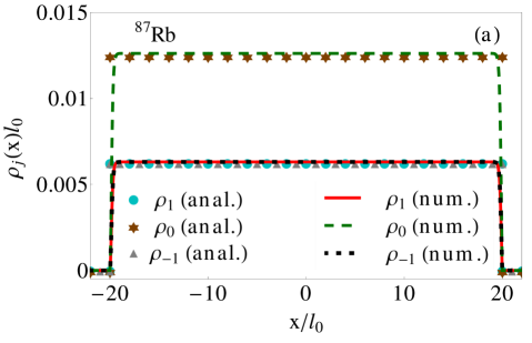
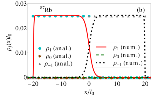
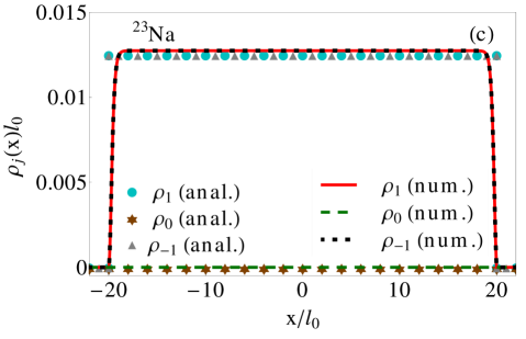
Figure 1: (Color online) (a) and (b) Analytical (anal.) and numerical (num.) densities $\rho_{j}(x)l_{0}$ of a condensate of ⁸⁷Rb atoms with $c_{0}=885.72l_{0}$ and $c_{2}=-4.09l_{0}$ in a 1D box of length $40l_{0}$. The SO coupling $\gamma=0$ and $0.5$ for (a) and (b), respectively. (c) The same for a condensate of ²³Na atoms with $c_{0}=241.28l_{0}$ and $c_{2}=7.76l_{0}$ in the presence of an arbitrary SO coupling. Both the densities and spatial coordinates in this figure are in dimensionless units.

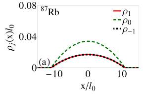
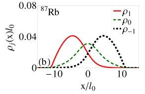
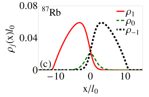
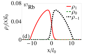
Figure 2: (Color online) Ground state structure of ⁸⁷Rb spinor BEC with $10000$ atoms with $\Omega=0$. The SO coupling $\gamma=0,~{}0.25,~{}0.5,~{}1$ for (a), (b), (c) and (d) respectively. All quantities in this figure are dimensionless.

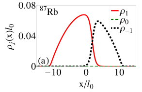
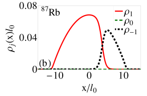
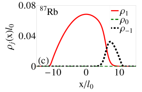
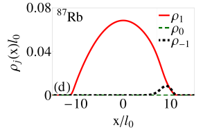
Figure 3: (Color online) Ground state structure of ⁸⁷Rb spinor BEC with $10000$ atoms with $\Omega=0$, $\gamma=1$. Both the density and spatial coordinates are plotted in dimensionless units. The magnetization ${\cal M}=0.25$, $0.5$, $0.75$, $0.95$ for (a), (b), (c) and (d) respectively.

Now, let us discuss the harmonically trapped spinor condensates. In Fig. 2 we present the densities of the ground state of $10000$ ⁸⁷Rb atoms with different SO coupling and without the Rabi term. Without the SO coupling, the ground state solution for ⁸⁷Rb is miscible and $\rho_{0}(x)>\rho_{1}(x)=\rho_{-1}(x)$ for zero magnetization (${\cal M}=0$) [viz. Fig. 2(a)], which is in qualitative agreement with the conclusion of the analytic study of the uniform system in Sec. III given by Eq. (29). If the number of atoms is sufficiently large, as the the SO coupling $\gamma$ is increased, the density $\rho_{0}$ starts decreasing slowly, which ultimately makes the system immiscible as is shown in Figs. 2(a) - (d). For a sufficiently strong SO coupling, $\rho_{0}$ becomes zero and there is a maximum of phase separation between the two remaining component densities $\rho_{1}(x)$ and $\rho_{-1}(x)$. This is again in agreement with the result of the analytic study on the uniform system given by Eq. (63), which predicts zero density for the $0$th component. However, if the number of atoms is smaller ($N\leq 1000$), the $0$th component again vanishes with the increase in SO coupling $\gamma$ above a critical value, but there is no phase separation between components $1$ and $-1$.

The state with $\rho_{0}(x)=0$ appears naturally with the increase of the SO coupling, and this in a zero magnetization case guarantees an equal number of atoms for the components $1$ and $-1$ resulting in $\rho_{1}(x)=\rho_{-1}(-x)$. It is interesting to study the fate of this state as the magnetization is increased (${\cal M}>0$). Keeping $\gamma=1$ and $\Omega=0$ fixed, one can change the relative proportion of $\rho_{1}$ and $\rho_{-1}$ by changing the magnetization ${\cal M}$, as is shown in Fig. 3 (a) - (d), maintaining $\rho_{0}(x)=0$. With increasing ${\cal M}$ the relative density of component $-1$ decreases and the system turns miscible from immiscible.

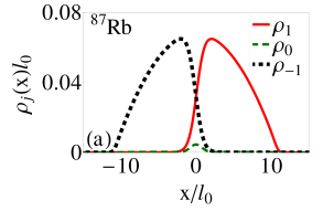
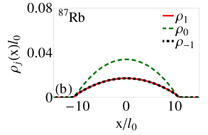
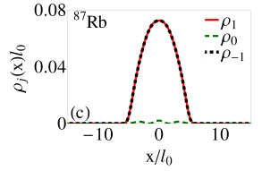
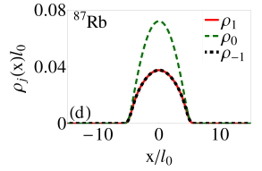
Figure 4: (Color online) Ground state structure of ⁸⁷Rb spinor BEC with $10^{4}$ atoms with (a) $N=10000$, $\Omega=0.1$, $\gamma=1$ (b) $N=10000$, $\Omega=1$, $\gamma=1$ (c) $N=1000$, $\Omega=0.1$, $\gamma=1$, and (d) $N=1000$, $\Omega=1$, $\gamma=1$. Both the density and spatial coordinates are plotted in dimensionless units. Magnetization ${\cal M}=0$ in all the cases.

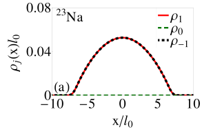
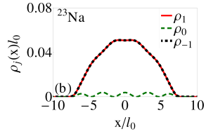
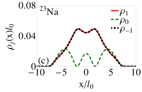
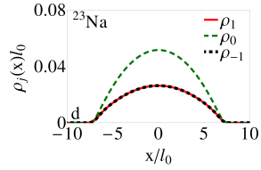
Figure 5: (Color online) Ground state structure of ²³Na spinor BEC with (a) $N=10000$, $\Omega=0$, $\gamma=1$, and also $\gamma=0$, (b) $N=10000$, $\Omega=0.5$, $\gamma=1$, (c) $N=10000$, $\Omega=1$, $\gamma=1$, (d) $N=10000$, $\Omega=1.5$, $\gamma=1$. Both the density and spatial coordinates are plotted in dimensionless units. The magnetization ${\cal M}=0$ is zero in all the cases.

We have also studied the effect of an increase in the the Rabi term $\Omega$ on the state with $\rho_{0}(x)=0$ [viz. Fig. 2 (d)] maintaining magnetization ${\cal M}=0$. As discussed in Sec. III, the Rabi term $\Omega$ favors miscibility of the system irrespective of the nature of the spin dependent interactions, while the SO-coupling term $\gamma$ favors a phase separation. Hence, when both $\gamma$ and $\Omega$ are non zero, there is a competition between these two terms as one favors phase separation, whereas the other favors miscibility. To illustrate this, in Figs. 4 (a) and (b) we plot the component densities for $\Omega=0.1$ and $1$, respectively, for $N=10000$ and $\gamma=1$. The increase in the Rabi term $\Omega$ from $0.1$ to $1$ has transformed a phase-separated state to a miscible state. For smaller number of atoms, say $N=1000$, we do not observe any phase separation with the increase in the SO coupling $\gamma$. Nevertheless, the increase in $\gamma$ leads to a decrease in $\rho_{0}$ as is shown in Fig. 4(c), where $\rho_{0}$ is negligible in comparison to overlapping $\rho_{1}$ and $\rho_{-1}$. Again as $\Omega$ is increased in this case, the density $\rho_{0}$ first increases and ultimately ends up being larger than those of other two components [viz., Fig. 4(d)].

In the case of the SO-coupled polar BEC ²³Na, we do not observe any phase separation consistent with the discussion of the uniform BEC in Sec. III. In the absence of the Rabi term ($\Omega=0$), the density profile in the presence and absence of the SO coupling are the same as is shown in Fig. 5 (a). The introduction of the Rabi term leads to a non-zero density of the $0$th component as shown in Fig. 5 (b) for $\Omega=0.5$. For both the ferromagnetic and polar BECs, in the presence of both SO coupling and Rabi terms, we observe a formation of structure in the ground state, where the $0$th component develops a train of dark notches as shown in Fig. 4(c) for ⁸⁷Rb and Figs. 5(b) and (c) for ²³Na. In ²³Na, an increase in the Rabi term $\Omega$ leads to an increase in $\rho_{0}(x)$ from 0, at the cost of $\rho_{1}(x)$ and $\rho_{-1}(x)$ as in the case of ⁸⁷Rb, and ultimately, ends up with a solution where $\rho_{0}(x)>\rho_{1}(x)=\rho_{-1}(x)$.

V Summary

We have studied the SO-coupled $F=1$ spinor BECs of ⁸⁷Rb (ferromagnetic) and ²³Na (antiferromagnetic or polar) atoms in quasi-1D traps. By comparing the energy of various competing structures for the SO-coupled spinor BEC in a 1D box, we have shown that any non-zero value of the SO coupling will lead to a phase separation between the $m_{F}=1$ and $m_{F}=-1$ components in the case of a ferromagnetic BEC in the absence of the Rabi term. On the other hand, for a polar BEC, SO coupling makes the miscible profile energetically more stable as compared to various possible phase-separated profiles. In the case of the trapped SO-coupled BECs, we have numerically studied the ground state structures. In the ferromagnetic case, above a critical number of atoms the BEC phase separates if the SO coupling strength exceeds a critical value in the absence of the Rabi term. The introduction of the Rabi term favors the miscibility for both the ferromagnetic and polar BECs. The present conclusions can be tested in experiments with present-day technology.

- (1) D. M. Stamper-Kurn, M. R. Andrews, A. P. Chikkatur, S. Inouye, H.-J. Miesner, J. Stenger, and W. Ketterle, Phys. Rev. Lett. 80 2027, (1998).
- (2) Y. Kawaguchi and M. Ueda, Phys. Rep. 520, 253 (2012).
- (3) L. Salasnich, A. Parola, and L. Reatto, Phys. Rev. A 65, 043614 (2002).
- (4) T. Ohmi, and K. Machida, J. Phys. Soc. Japan, 67, 1822 (1998).
- (5) T. L. Ho, Phys. Rev. Lett. 81, 742 (1998).
- (6) J. Higbie and D. M. Stamper-Kurn, Phys. Rev. Lett. 88, 090401 (2002); T. L. Ho and S. Zhang, Phys. Rev. Lett. 107, 150403 (2011); Y. Deng, J. Cheng, H. Jing, C. P. Sun, and S. Yi, Phys. Rev. Lett. 108, 125301 (2012); J. Radic, T. A. Sedrakyan, I. B. Spielman, and V. Galitski, Phys. Rev. A 84, 063604 (2011);.
- (7) Y. A. Bychkov and E. I. Rashba, J. Phys. C 17, 6039 (1984).
- (8) G. Dresselhaus, Phys. Rev. 100, 580 (1955).
- (9) X.-J. Liu, M. F. Borunda, X. Liu, and J. Sinova, Phys. Rev. Lett. 102, 046402 (2009).
- (10) Y.-J. Lin, K. Jiménez-García, and I. B. Spielman, Nature 471, 83 (2011).
- (11) V. Galitski and I. B. Spielman, Nature 494, 49 (2013).
- (12) J.-Y. Zhang, S.-C. Ji, Z. Chen, L. Zhang, Z.-D. Du, B. Yan, G.-S. Pan, B. Zhao, Y.-J. Deng, H. Zhai, S. Chen, and J.-W. Pan, Phys. Rev. Lett. 109, 115301 (2012); C. Qu, C. Hamner, M. Gong, C. Zhang, and P. Engels, Phys. Rev. A 88, 021604(R) (2013); M. Aidelsburger, M. Atala, and S. Nascimb´ene et al., Phys. Rev. Lett. 107, 255301 (2011); Z. Fu, P. Wang, and S. Chai, L. Huang, and J. Zhang, Phys. Rev. A 84, 043609 (2011).
- (13) G. Juzeliūnas, J. Ruseckas, and J. Dalibard, Phys. Rev. A 81, 053403 (2010); J. Dalibard et al., Rev. Mod. Phys. 83, 1523 (2011).
- (14) P. Wang, Z.-Q. Yu, Z. Fu, J. Miao, L. Huang, S. Chai, H. Zhai, and J. Zhang, Phys. Rev. Lett. 109, 095301 (2012); L. W. Cheuk, A. T. Sommer, Z. Hadzibabic, T. Yefsah, W. S. Bakr, and M. W. Zwierlein, Phys. Rev. Lett. 109, 095302 (2012).
- (15) H. Wang, Int. J. of Computer Math. 84, 925 (2007).
- (16) W. Bao and F. Y. Lim, Siam J. Sci. Comp. 30, 1925 (2008); F. Y. Lim and W. Bao, Phys. Rev. E 78, 066704 (2008).
- (17) C. Wang, C. Gao, C-M Jian, and H. Zhai, Phys. Rev. Lett. 105, 160403 (2010); A. Aftalion and P. Mason, Phys. Rev. A 88, 023610 (2013); R. Gupta, G. S. Singh, and J. Bosse, Phys. Rev. A 88, 053607 (2013); Q.-Q. Lu and D. E. Sheehy, Phys. Rev. A 88, 043645 (2013).
- (18) T. D. Stanescu, B. Anderson, and V. Galitski, Phys. Rev. A 78, 023616 (2008); C.-J Wu and I. Mondragon-Shem, X.-F. Zhou Chin. Phys. Lett. 28, 097102 (2011); Q. Zhou and X. Cui, Phys. Rev. Lett. 110, 140407 (2013); S. Gopalakrishnan, A. Lamacraft, and P. M. Goldbart, Phys. Rev. A 84, 061604(R) (2011); H. Hu, B. Ramachandhran, H. Pu, and X.-J. Liu, Phys. Rev. Lett. 108, 010402 (2012); B. Ramachandhran, B. Opanchuk, X.-J. Liu, H. Pu, P. D. Drummond, and H. Hu, Phys. Rev. A 85, 023606 (2012); S. Sinha, R. Nath, and L. Santos, Phys. Rev. Lett. 107, 270401 (2011); T. Ozawa and G. Baym, Phys. Rev. A 85, 013612 (2012).
- (19) Z. F. Xu, Y. Kawaguchi, L. You, and M. Ueda, Phys. Rev. A 86, 033628 (2012); S.-W. Song, Y.-C. Zhang, H. Zhao, X. Wang, and W.-M. Liu, Phys. Rev. A 89, 063613 (2014); P.-S. He, Y.-H. Zhu, and W.-M. Liu Phys. Rev. A 89, 053615 (2014); Y. Deng, J. Cheng, H. Jing, and S. Yi, Phys. Rev. Lett. 112, 143007 (2014); K. Riedl, C. Drukier, P. Zalom, and P. Kopietz, Phys. Rev. A 87, 063626 (2013); T. Kawakami, T. Mizushima, and K. Machida, Phys. Rev. A 84, 011607 (2011); Z. F. Xu, R. Lü, and L. You, Phys. Rev. A 83, 053602 (2011); S.-K. Yip, Phys. Rev. A 83, 043616 (2011); S.-W. Su, I.-K. Liu, Y.-C. Tsai, W. M. Liu, and S.-C. Gou, Phys. Rev. A 86, 023601 (2012); Y. Zhang, L. Mao, and C. Zhang, Phys. Rev. Lett. 108, 035302 (2012); S.-W. Song, Y.-C. Zhang, L. Wen, and H. Wang, J. Phys. B 46, 145304 (2013).
- (20) E. Ruokokoski, J. A. M. Huhtamäki, and M. Möttönen, Phys. Rev A 86, 051607(R) (2012).
- (21) J. Larson, J.-P. Martikainen, A. Collin, and E. Sjöqvist, Phys. Rev. A 82, 043620 (2010).
- (22) M. Merkl, A. Jacob, F. E. Zimmer, P. Öhberg, and L. Santos, Phys. Rev. Lett. 104, 073603 (2010).
- (23) T. Ozawa, L. P. Pitaevskii, and S. Stringari, Phys. Rev. A 87, 063610 (2013); D. W. Zhang, J. P. Chen, C. J. Shan, Z. D. Wang, and S. L. Zhu, Phys. Rev. A 88, 013612 (2013); Q. Zhu, C. Zhang and B. Wu, Europhys. Lett. 100, 50003 (2012); D. Toniolo and J. Linder, Phys. Rev. A 89, 061605(R) (2014).
- (24) M. A. Garcia-March, G. Mazzarella, L. Dell’Anna, B. Juliá-Díaz, L. Salasnich, and A. Polls, Phys. Rev. A 89, 063607 (2014).
- (25) A. L. Fetter, Phys. Rev. A 89, 023629 (2014). X. F. Zhou, J. Zhou, and C. Wu, Phys. Rev. A 84, 063624 (2011); Z.-F. Xu, S. Kobayashi, and M. Ueda, Phys. Rev. A 88, 013621 (2013); C.-F. Liu, Y.-M. Yu, S.-C. Gou, and W.-M. Liu, Phys. Rev. A 87, 063630 (2013).
- (26) H. Sakaguchi, Ben Li, and B. A. Malomed, Phys. Rev. E 89, 032920 (2014); Y. Xu, Y. Zhang, and B. Wu, Phys. Rev. A 87, 013614 (2013); O. Fialko, J. Brand, and U. Z¨ulicke, Phys. Rev. A 85, 051605(R) (2012).
- (27) F. Zhou, Phys. Rev. Lett. 87, 080401 (2001); S. Yi, Ö. E. Müstecaplioglu, C. P. Sun, and L. You, Phys. Rev. A 66, 011601(R) (2002); W. Zhang, S. Yi, and L. You, New J. Phys. 5, 77 (2003); K. Murata, H. Saito, and M. Ueda, Phys. Rev. A 75, 013607 (2007).
- (28) M. Matuszewski, T. J. Alexander, and Y. S. Kivshar, Phys. Rev. A 80, 023602 (2009).
- (29) M. Matuszewski, Phys. Rev. A 82, 053630 (2010).
- (30) P. Ao and S. T. Chui, Phys. Rev. A 58, 4836 (1998); P. Facchi, G. Florio, S. Pascazio, and F. V. Pepe, J. Phys. A: Math. Theor. 44 505305 (2011).
- (31) Z. Lan and P. Öhberg, Phys. Rev. A89, 023630 (2014).
- (32) Y. Li, G. I. Martone, L. P. Pitaevskii, and S. Stringari, Phys. Rev. Lett. 110, 235302 (2013); Y. Zhang and C. Zhang, Phys. Rev. A 87, 023611 (2013); L. Salasnich and B. A. Malomed, Phys. Rev. A 87, 063625 (2013); D. A. Zezyulin, R. Driben, V. V Konotop, and B. A. Malomed, Phys. Rev. A 88, 013607 (2013); Y. Cheng, G. Tang, and S. K. Adhikari, Phys. Rev. A 89, 063602 (2014).
- (33) S. Gautam and D. Angom, J. Phys. B 44, 025302 (2011); S. Gautam and D. Angom, J. Phys. B 43, 095302 (2010).
- (34) T. Isoshima, K. Machida, and T. Ohmi, J. Phys. Soc. Japan 70, 1604 (2001).
- (35) P. Muruganandam and S. K. Adhikari, Comput. Phys. Commun. 180, 1888 (2009); D. Vudragovic, I. Vidanovic, A. Balaz, P. Muruganandam, and S. K. Adhikari. Comput. Phys. Commun. 183, 2021 (2012).